ABSTRACT
ROLLINS, CHAD ERIC. Development of Multiphase Computational Fluid Dynamics Solver in OpenFOAM. (Under the direction of Hong Luo.)
From the viewpoint of an increase in energy demand, a shortage of fossil fuels and changes in the climate on the global scale, nuclear power has the ability to represent a part of the solution to the energy and environmental problems we are facing currently. However, there are still problems that need solutions regarding the management of the nuclear waste, public opinion of nuclear power and public safety surrounding nuclear power plants during accidents (as proved via the fairly recent Fukushima accident). The interest in improving the safety and reliability of nuclear power plants through researching and developing advancements to nuclear energy production is strong and still ongoing. In this context, the basic motivation for this work is based on the need to evaluate and improve the current strategies for CFD modeling of two-phase Eulerian flows in boiling channels. The modeling of these types of problems presents several challenges. The major challenge lies in the presence of the many closure models that are all tightly non-linearly coupled in the solution process. Other challenges are that many of the closure models are empirically determined using relatively small sets of flow conditions; thus, the sensitivity & accuracy of these closure models in the wide range of flow conditions that need to be modeled for a general multiphase CFD solver. Also, there is a distinct lack of detailed experimental results for quantities of interest at the operating conditions of a interest (i.e. high pressure boiling cases).
of open-source code, have the added benefit of being able to include sensitivity analysis and uncertainty quantification techniques on quantities of interest in the simulation. The relevance of these first steps in the development, in terms of usage for accident scenarios for PWRâ ˘A ´Zs which requires modeling the critical heat flux mechanism of departure from nucleate boiling, of the testing platform is that it gives users the ability to test all the closure and algorithm methods for stability and accuracy in a structured and efficient manner before the extreme case of DNB.
© Copyright 2018 by Chad Eric Rollins
Development of Multiphase Computational Fluid Dynamics Solver in OpenFOAM
by
Chad Eric Rollins
A dissertation submitted to the Graduate Faculty of North Carolina State University
in partial fulfillment of the requirements for the Degree of
Doctor of Philosophy
Mechanical Engineering
Raleigh, North Carolina
2018
APPROVED BY:
Jack Edwards Nam Dinh
Igor Bolotnov Hong Luo
DEDICATION
BIOGRAPHY
ACKNOWLEDGEMENTS
TABLE OF CONTENTS
LIST OF TABLES . . . viii
LIST OF FIGURES. . . ix
Chapter 1 INTRODUCTION. . . 1
1.1 Background . . . 1
1.2 Subcooled Boiling . . . 2
1.3 CFD Methodology . . . 5
1.4 OpenFOAM . . . 6
1.5 Motivation . . . 9
Chapter 2 GOVERNING EQUATIONS . . . 11
2.1 Conservation of Mass . . . 11
2.2 Conservation of Momentum . . . 15
2.3 Conservation of Energy . . . 18
Chapter 3 TURBULENCE CLOSURE MODELS . . . 22
3.1 Continuous Phase Turbulence Model . . . 22
3.2 Dispersed Phase Turbulence Model . . . 24
3.3 Wall Function Models . . . 25
Chapter 4 INTERFACIAL MOMENTUM TRANSFER CLOSURE MODELS . . . 27
4.1 Interfacial Drag Models . . . 28
4.1.1 Constant Drag Model . . . 29
4.1.2 Schiller & Naumann Drag Model . . . 29
4.1.3 Ishii & Zuber Drag Model . . . 29
4.1.4 Ergun Drag Model . . . 30
4.1.5 Gibilaro Drag Model . . . 30
4.1.6 Gidaspow Drag Model . . . 31
4.1.7 Syamlal & O’Brien Drag Model . . . 32
4.1.8 Wen & Yu Drag Model . . . 32
4.1.9 Tomiyama Drag Model . . . 33
4.2 Interfacial Lift Models . . . 34
4.2.1 Constant Lift Model . . . 34
4.2.2 Rusche Lift Model . . . 35
4.2.3 Tomiyama Lift Model . . . 35
4.3 Interfacial Wall Lubrication Models . . . 36
4.3.1 Constant Wall Lubrication Model . . . 36
4.3.2 Antal Wall Lubrication Model . . . 36
4.3.4 Hosokawa Wall Lubrication Model . . . 37
4.3.5 Tomiyama Wall Lubrication Model . . . 38
4.4 Interfacial Turbulence Dispersion Models . . . 39
4.4.1 Burns Turbulence Dispersion Model . . . 39
4.4.2 Gosman Turbulence Dispersion Model . . . 39
4.4.3 Lopez De Bertodano Turbulence Dispersion Model . . . 40
4.5 Interfacial Virtual Mass Models . . . 40
4.5.1 Constant Virtual Mass Model . . . 41
Chapter 5 INTERFACIAL DIAMETER CLOSURE MODELS . . . 42
5.1 Constant Diameter Model . . . 42
5.2 Thermal Diameter Model . . . 42
5.3 Iso-thermal Diameter Model . . . 43
5.4 Interfacial Area Concentration Model . . . 43
5.4.1 Break-up Source Term . . . 45
5.4.1.1 Hibiki & Ishii Break-up Model . . . 45
5.4.1.2 Wu et al. Break-up Model . . . 46
5.4.1.3 Yao & Morel Break-up Model . . . 47
5.4.1.4 Nguyen et al. Break-up Model . . . 47
5.4.2 Coalescence Source Term . . . 47
5.4.2.1 Hibiki & Ishii Coalescence Model . . . 48
5.4.2.2 Wu et al. Coalescence Model . . . 49
5.4.2.3 Yao & Morel Coalescence Model . . . 49
5.4.2.4 Nguyen et al. Coalescence Model . . . 50
Chapter 6 PHASE CHANGE CLOSURE MODELS. . . 51
6.1 Interfacial Heat Transfer Coefficient Closure Models . . . 51
6.1.1 Ranz & Marshall Model . . . 51
6.1.2 Chen & Mayinger Model . . . 52
6.1.3 Wolfert et al. Model . . . 53
6.2 Condensation Closure Model . . . 53
6.3 Wall Heat Flux Partitioning Closure Model . . . 53
6.3.1 Wall Heat Flux Partitioning . . . 55
6.3.2 Wall Area Fraction Models . . . 58
6.3.3 Bubble Area Influence Factor Model . . . 59
6.3.4 Bubble Departure/Detachment Diameter Model . . . 59
6.3.5 Bubble Departure Frequency Model . . . 60
6.3.6 Single-phase Heat Transfer Coefficient Model . . . 60
6.3.7 Two-phase Heat Transfer Coefficient Model . . . 61
6.3.8 Nucleation Site Density Models . . . 62
6.5 Volumetric Heat Source Closure Model . . . 64
Chapter 7 NUMERICS . . . 66
7.1 Description . . . 66
7.2 PISO Algorithm & Pressure-Velocity Coupling . . . 68
7.3 Solution Algorithm . . . 72
7.4 Testing Platform . . . 74
Chapter 8 NUMERICAL RESULTS . . . 75
8.1 Ransom’s Faucet Problem . . . 75
8.2 Air-to-Water Shocktube Problem . . . 83
8.3 Blasius Flat Plate Problem . . . 85
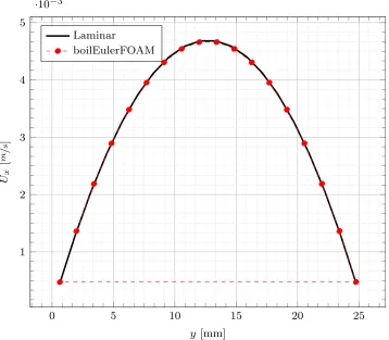
8.4 Laminar Flow in a Pipe Problem . . . 87
8.5 Purdue Experiments . . . 89
8.6 MT-Loop Experiments . . . 99
8.7 Bartolomej Experiments . . . 109
8.8 DEBORA Experiments . . . 122
8.9 MIT Boiling Test Facility Experiments . . . 130
Chapter 9 CONCLUSIONS . . . 141
BIBLIOGRAPHY . . . 143
APPENDIX . . . 149
Appendix A OpenFOAM Spatial & Temporal Discretization . . . 150
LIST OF TABLES
Table 8.1 Ransom’s Faucet Problem Initial Conditions . . . 76
Table 8.2 Air-to-Water Shocktube Problem Initial Conditions . . . 83
Table 8.3 Blasius Flat Plate Problem Setup . . . 86
Table 8.4 Laminar Flow in a Pipe Problem Setup . . . 88
Table 8.5 Purdue Experiments - Brief Experimental Setup . . . 91
Table 8.6 Purdue Experiments - Flow Structure Development Study . . . 91
Table 8.7 Purdue Experiments - Fully Developed Flow Study . . . 92
Table 8.8 Purdue Experiments - Selected Experiments . . . 93
Table 8.9 Purdue Experiments - Thermo-physical Properties . . . 94
Table 8.10 Purdue Experiments - Boundary Conditions . . . 95
Table 8.11 Purdue Experiments - Star-CCM+Closure Modeling Summary . . . 96
Table 8.12 Purdue Experiments - Reference Closure Model Summary . . . 97
Table 8.13 MT-Loop Experiments - Brief Experimental Setup . . . 101
Table 8.14 MT-Loop Experiments - Selected Experiments . . . 103
Table 8.15 MT-Loop Experiments - Thermo-physical Properties . . . 104
Table 8.16 MT-Loop Experiments - Boundary Conditions . . . 105
Table 8.17 MT-Loop Experiments - Star-CCM+Closure Modeling Summary . . . 106
Table 8.18 MT-Loop Experiments - Reference Closure Model Summary . . . 107
Table 8.19 Bartolomej Experiments - Selected Experiments . . . 111
Table 8.20 Bartolomej Experiments - Available Experimental Data . . . 111
Table 8.21 Bartolomej Experiments - Thermo-physical Properties . . . 112
Table 8.22 Bartolomej Experiments - Boundary Conditions . . . 113
Table 8.23 Bartolomej Experiments - BART07 Setup Summary . . . 115
Table 8.24 Bartolomej Experiments - Efficiency Study . . . 122
Table 8.25 DEBORA Experiments - Brief Experimental Setup . . . 124
Table 8.26 DEBORA Experiments - Selected Experiments . . . 124
Table 8.27 DEBORA Experiments - Thermo-physical Properties . . . 125
Table 8.28 DEBORA Experiments - Boundary Conditions . . . 126
Table 8.29 DEBORA Experiments - BART07 Setup Summary . . . 128
Table 8.30 MIT Experiments - Available Experimental Data . . . 132
Table 8.31 MIT Experiments - Test Facility Dimensions and Properties . . . 133
Table 8.32 MIT Experiments - Potential Operating Conditions . . . 133
Table 8.33 MIT Experiments - Summary of Experiments . . . 134
Table 8.34 MIT Experiments - MIT03 Thermo-physical Properties . . . 134
Table 8.35 MIT Experiments - Boundary Conditions . . . 135
LIST OF FIGURES
Figure 1.1 Flow patterns and heat transfer regimes in a vertical pipe with upward
flow[5, 21, 41] . . . 3
Figure 1.2 Boiling curve - Influence of wall heat flux on wall superheat[5, 21, 41] 4 Figure 1.3 OpenFOAM Overall Structure . . . 8
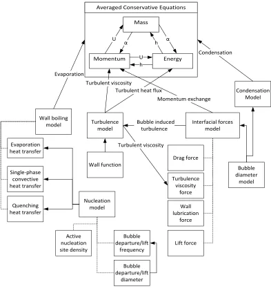
Figure 7.1 Closure Model Network . . . 67
Figure 7.2 Solution Algorithm . . . 73
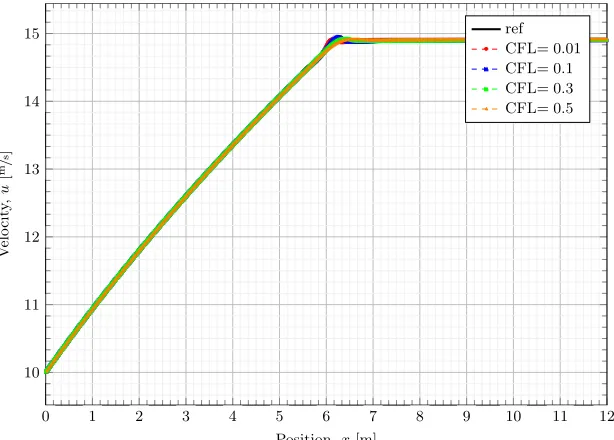
Figure 8.1 Ransom’s Faucet Problem PISO Algorithm Grid Refinement - Void Fraction Comparison . . . 77
Figure 8.2 Ransom’s Faucet Problem PISO Algorithm Grid Refinement - Velocity Comparison . . . 78
Figure 8.3 Ransom’s Faucet Problem PIMPLE Algorithm Grid Refinement - Void Fraction Comparison . . . 78
Figure 8.4 Ransom’s Faucet Problem PIMPLE Algorithm Grid Refinement - Ve-locity Comparison . . . 79
Figure 8.5 Ransom’s Faucet Problem PIMPLE Algorithm CFL Refinement - Void Fraction Comparison . . . 80
Figure 8.6 Ransom’s Faucet Problem PIMPLE Algorithm CFL Refinement - Ve-locity Comparison . . . 80
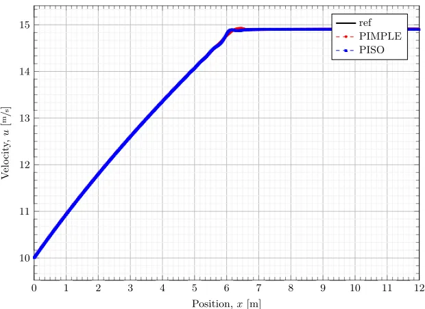
Figure 8.7 Ransom’s Faucet Problem PIMPLE & PISO Algorithm - Void Fraction Comparison . . . 81
Figure 8.8 Ransom’s Faucet Problem PIMPLE & PISO Algorithm - Velocity Com-parison . . . 82
Figure 8.9 Ransom’s Faucet Problem PIMPLE Algorithm Comparison - Void Fraction . . . 82
Figure 8.10 Air-to-Water Shocktube CFL=0.5 Grid Refinement . . . 84
Figure 8.11 Air-to-Water Shocktube 100 cells with varying CFL Comparison . . . 85
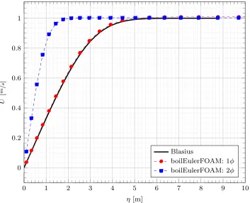
Figure 8.12 Blasius Flat Plate x-direction Velocity Comparison . . . 87
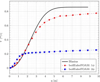
Figure 8.13 Blasius Flat Plate y-direction Velocity Comparison . . . 88
Figure 8.14 Laminar Flow in a Pipe Comparison . . . 89
Figure 8.15 Purdue Experiment Geometry . . . 90
Figure 8.16 Purdue Experiments - Flow Pattern Map . . . 92
Figure 8.17 Purdue Experiments - PU01 Star-CCM+Comparison . . . 98
Figure 8.18 Purdue Experiments - PU01 Grid Refinement . . . 99
Figure 8.19 Purdue Experiments - PU01 Void Fraction Comparison . . . 100
Figure 8.20 Purdue Experiments - PU01 Interfacial Area Conc. Comparison . . . . 101
Figure 8.22 MT-Loop Experiments - Matrix of superficial velocities and Capillary Groups[45] . . . 102 Figure 8.23 MT-Loop Experiments - Flow Pattern Map . . . 103 Figure 8.24 MT-Loop Experiments MT017 Comparison - Coefficient Ratio 5 . . . 107 Figure 8.25 MT-Loop Experiments MT017 Comparison - Coefficient Ratio 1.5 . . 108 Figure 8.26 MT-Loop Experiments MT061 Void Fraction Comparison . . . 109 Figure 8.27 Bartolomej Experiments - Test Section Geometry . . . 110 Figure 8.28 Bartolomej Experiments - BART07 Wall Superheat Comparison . . . . 116 Figure 8.29 Bartolomej Experiments - BART07 Liquid Subcooling Comparison . 116 Figure 8.30 Bartolomej Experiments - BART07 Void Fraction Comparison . . . 117 Figure 8.31 Bartolomej Experiments - BART07 Wall Superheat Grid Refinement
Comparison . . . 117 Figure 8.32 Bartolomej Experiments - BART07 Liquid Subcooling Grid
Refine-ment Comparison . . . 118 Figure 8.33 Bartolomej Experiments - BART07 Radial Liquid Subcooling Grid
Refinement Comparison at Outlet . . . 118 Figure 8.34 Bartolomej Experiments - BART07 Void Fraction Grid Refinement
Comparison . . . 119 Figure 8.35 Bartolomej Experiments - BART07 Radial Void Fraction Grid
Refine-ment Comparison at Outlet . . . 120 Figure 8.36 Bartolomej Experiments - BART07 Interfacial Bubble Diameter
Clo-sure Wall Superheat Comparison . . . 120 Figure 8.37 Bartolomej Experiments - BART07 Interfacial Bubble Diameter
Clo-sure Liquid Subcooling Comparison . . . 121 Figure 8.38 Bartolomej Experiments - BART07 Interfacial Bubble Diameter
Clo-sure Void Fraction Comparison . . . 121 Figure 8.39 DEBORA Experiments - Test Section Geometry (Krepper and Rzehak,
2011)[33] . . . 123 Figure 8.40 DEBORA Experiments - DEB01 Void Fraction Comparison . . . 129 Figure 8.41 DEBORA Experiments - DEB01 Bubble Diameter Comparison . . . 129 Figure 8.42 DEBORA Experiments - DEB01 Liquid Temperature Comparison . . 130 Figure 8.43 MIT Experiments - Experimental Geometry[24] . . . 131 Figure 8.44 MIT Experiments - Heated Quartz Section Geometry[24] . . . 132 Figure 8.45 MIT Experiments - MIT03 Area Averaged Wall Superheat vs Power at
Heated Section . . . 138 Figure 8.46 MIT Experiments - MIT03 Area Averaged Void Fraction vs Power at
Heated Section . . . 138 Figure 8.47 MIT Experiments - MIT03 Area Averaged Nucleation Site Density vs
Power at Heated Section . . . 139 Figure 8.48 MIT Experiments - MIT03 Area Averaged Bubble Departure Frequency
Chapter 1
INTRODUCTION
1.1
Background
From the viewpoint of an increase in energy demands, a shortage of fossil fuels and changes in the climate on the global scale, nuclear power has the ablility to represent a part of the solution to the energy and environmental problems that we are facing currently. Some of the advantages of nuclear power are,
• Lack of greenhouse gas emissions into the atmosphere that contribute to the climate change.
• Low cost per kWh of electricity production.
• Small power plants (relatively) produce large amounts of electricity due to the high energy density of the nuclear fuel.
• Is a very mature and reliable technology (thousands of cumulative nuclear reactor years of comericial operation across dozens of countries in the world) in comparison to renewable energy sources that lack a consistancy of supply and also, in order to be used on a larger scale, require further developments and research.
and developing advancements to nuclear energy production is strong and still ongoing. In this context, this thesis deals with the development and validation of an in-house two-phase computational fluid dynamics (CFD) solver with phase change capabilities (e.g. subcooled boiling) in OpenFoam.
1.2
Subcooled Boiling
2 Introduction
Figure 1.1: Flow patterns and heat transfer regimes in a heated channel, from Anglart [1]
defense-in-depth principle. At low thermodynamic equilibrium qualities, which is the in a PWR core or the lower part of a BWR core, the CHF occurs when the boiling mechanism evolves from nucleate boiling to film boiling which is referred to as Departure from Nucleate Boiling (DNB), and represented by the point C in Figure 1.2. DNB sets an upper limit to the power that can be generated by the fuel.
In the case of PWR, even if this limit seems of no concern during normal operation, it is essential to ensure that safety margins will also be respected in case of transients, incidents or accidents. Indeed, subcooled boiling can even occur in the higher part of a PWR core, and it would generate a lithium borate deposition which a↵ects significantly the power distribution. This phenomenon is called axial o↵set anomaly (AOA). The nuclear safety analysis of BWR is also influenced by the system reactivity. Subcooled nucleate boiling causes a highly inhomogeneous void fraction distribution in the axial direction (along the flow) since the channel is heated, but also in the cross-sectional direction due to the migration of steam bubbles. The presence of bubbles and their distribution induces a non-negligible reactivity feedback. Consequently, it is crucial to be able to predict the void fraction distribution if one wants to couple thermal-hydraulics and neutronics. The codes used today for this purpose are still old system level codes with a quasi one-dimensional representation of the flow and heat transfer in the core. Clearly there is a need for advanced models of the complex physics.
1.3
Computational fluid dynamics (CFD)
Reproducing the flow conditions of a power plant in an experimental facility is very difficult and expensive. Figure 1.1Flow patterns and heat transfer regimes in a vertical pipe with upward flow[5, 21, 41]
rate and coefficient. When the bulk of the liquid reaches the saturation temperature, the saturated nucleate boiling regime starts, during which many other different flow patterns can be observed (such as slug, churn and anular flow). Dry-out occurs when the liquid film along the wall of the heated channel during anular flow dissappears due to evapo-ration. This results in a high increase in wall temperature due to the deterioration of the heat transfer coefficient from the direct contact between the vapor and the heated walls. A different thermal crisis type is the so-called Departure from Nucleate Boiling (DNB) and this can occur with low mass flow rates or large heat fluxes so that the heat flux at the wall is larger than the Critical Heat Flux (CHF). During DNB the boiling mechanism changes from nucleate boiling (very high heat transfer coefficient) to film boiling where a vapor
Objectives of the work 3
Figure 1.2:Boiling curve, influence of the wall heat flux on the wall superheat, from Anglart [1]
• Pre-processing: the geometry is defined and divided into discrete cells (the mesh), the initial and boundary conditions as well as physical properties of the fluid are set up
• Solver: the governing equations are discretized (both in time and space) and solved applying an iterative process
• Post-processing: the results are displayed thanks to various user-friendly visual tools
OpenFOAM R (OF) is one of many existing CFD software packages available on the market. Its creation was initiated at the Imperial College in London in the late 1980’s and the first version was released in 2004. OF is provided with many discretization schemes and a certain number of predefined solvers that can be applied for various fluid dynamics problems. OF has many advantages:
• object-oriented: one can select solvers, reflecting the physics one wants to model, independantly from discretization schemes or cases on which to apply the solvers. This feature gives OF en enhanced flexibility.
• open-source: the code is transparent and one can easily add or modify equations to create or improve solvers. This characteritic makes OF very interesting from an academic and research point of view.
• free of charge: there is no license restriction and companies can use OF without paying any fee.
1.4 Objectives of the work
The present study aims to develop a new solver for subcooled nucleate boiling within the OpenFOAM framework. A multi-dimensional modeling using a two-fluid Eulerian approach has been chosen. This work comports two main development stages. The first one is dedicated to the development of an adiabatic solver without phase changemyTwoPhaseEulerFoamAdiabatic, and after validation of the latter, it has been further developed to account for boiling and subsequent condensation. This last version constitutes a new solver calledmyTwoPhaseEulerFoamBoiling. In addition to standard conservation equations, a one-group interfacial area concentration transport equation has been implemented and formyTwoPhaseEulerFoamBoilingboiling has been modeled according to Kurul and Podowski [19]. The solvers will be respectively tested and validated against adiabatic and diabatic experiments of vertical upward flows in cylindrical pipes.
These solvers should be taken as a basis for further implementation. They constitutes a skeleton for subcooled nucleate boiling modeling in OpenFOAM but do not intend to be complete and sophisticated. The solvers Figure 1.2Boiling curve - Influence of wall heat flux on wall superheat[5, 21, 41]
layer prevents liquid from reaching the heated walls leading to a sudden decrease of the heat transfer coefficient. The sudden decrease in the heat transfer coefficient causes a massive spike in the wall temperature which can eventually cause fuel rods damage and, in a worst case scenario, it can cause a core melt-down. DNB is a CHF mechanism that occur both in Pressurized Water Reactors (PWR) and in the lower part of Boiling Water Reactors (BWR) during various accidents. Therefore, a clear understanding of two-phase flows, of the boiling mechanisms, and simulating both accurately and efficiently is of huge interest in the nuclear industry.
In fact, a correct modeling of subcooled boiling can be considered as a first step towards better CHF predictions in nuclear reactors during accidents. Furthermore, a more correct understanding and modeling of subcooled boiling can,
• Improve the simulation/prediction of deposition of impurities along the axis of the core that can cause an issue refered to as Axial Offset Anomaly (AOA) in PWR cores.
• Improve the coupled neutronic & thermal-hydraulic calculations because the raidal and axial distribution of void fractions directly influences the reactivity of the core which provides reactivity feedbacks that cannot be neglected.
by subcooled boiling[26]. The solver described in this thesis is designed for dealing with both subcooled boiling flows and adiabatic bubbly flows.
1.3
CFD Methodology
In order to predict the parameters in two-phase flows and there multidimensional distri-butions, a Computational Fluid Dynamics (CFD) methodology is used in this study. The CFD methodology allows one to obtain approximate numerical solutions of fluid flows through discretization. Discretization is replacing the set of coupled differential equations describing the flow by a set of algebraic equations which can be solved by the use of a computer. The CFD methodology became more and more important with the increase of computational power and it now represents an significant engineering tool that allows one to not have to rely on the usage of experimental studies and empirical correlations for modeling fluid flow but, instead substituting them with more generally applicable methods. It is also a much cheaper way of solving some engineering problems. However, CFD models still require to be validated against experimental data before their usage can be defended and this is one of the purposes behind the work of this thesis.
CFD, much like any other numerical methodology, consists of a model (e.g. a mathe-matical representation of a physical phenomena that typically neglects the less important features to keep it as simple as possible) and a solution procedure in order to obtain an approximate numerical solution from the model. The modeling in CFD starts from the Navier-Stokes equations for fluid flows. These equations are valid for every flow regime (e.g. laminar or turbulent) but they are very difficult to solve numerically, especially for high Reynolds number flows which is one of the areas of interest in this study. Simplifica-tions of the equaSimplifica-tions and modeling assumpSimplifica-tions are required to reduce the complexity of the mathematical model as well as the computational cost of the simulations. If the Navier-Stokes equations are also solved without any manipulation it is by so-called Direct Numerical Simulation (DNS). DNS requires extremely high resolution modeling in order to resolve all the temporal and spatial scales. This is a huge computational effort. This means that the use of DNS is limited to the simulations of low Reynolds number flows and extremely small physical domains for any practical purposes.
suit-able averaging procedure of the the microscopic governing equations (e.g. Navier-Stokes equations) that is described more in detail in[49, 64]. This suitable averaging procedure simplifies the complexity of the set of equations by significantly reducing the required com-putational effort; however, it also introduces additional terms in the averaged equations which require closure laws (e.g. the Reynolds stress in the momentum conservation equa-tion). While the Navier-Stokes equations are well established, the closure laws especially for two-phase flows are not generally applicable to all situations, require further development and are still an object of much debate among scientists. This means that the validation of such models against experimental data is still necessary.
In this work a two-fluid model is used and both phases (continuous and dispersed phase) are modeled with Eulerian conservation equations (e.g. what is refered to as an Euler-Euler model). This means that each phase is treated as a continuum with the use of Reynolds Averaged Navier-Stokes (RANS) equations along with the introduction of the volume phase fractions in the equations. As previously mentioned, the averaging procedure introduces new terms in the momentum equations such as,
• The Reynolds stress which requires a two-phase turbulence model.
• The interfacial momentum transfer term which models the transfer of momentum between the phases (the formulation and modeling of this term needs to be improved since is not well established yet).
• The interfacial diameter term that models the bubble sizes and significantly affects the behavious of the momentum transfer terms.
• The wall heat flux partitioning schemes and the various mechanistic models used to model the volumetric mass and energy source terms.
These closure laws are the weak points of the two-fluid model approach and therefore will be a topic of future study from this work.
1.4
OpenFOAM
further developed and the number of users has increased drastically in recent years. This is thought to be due to three main advantages of using OpenFOAM,
• The software is obtained free of charge.
• The software is open-source, which means that the code can easily be modified in order to improve existing solvers as well as be reviewed by peers.
• The software is heavily object-oriented and this object-orientation allows users to introduce new models and solvers (user-selectable) without changing the main source code and independently from the discretization scheme used. This provides awesome flexibility and a simplicity of use.
The programming language is C++and the software is designed to run on Linux systems. OpenFOAM uses Finite Volume Methodology (FVM) in order to discretize and solve com-plex fluid dynamics problems. The first step of any CFD discretization is to create a 3-D volume of interest and divide it into small volumes or cells. Thus, obtaining the so-called mesh. After the mesh is created the initial and boundary conditions necessary for solving the conservation equations are defined and applied to the geometry. After, OpenFOAM discretizes the modeled equations using the previously built mesh. In CFD there are three main discretization schems or approaches used,
• Finite Difference Method (FDM) - uses conservation equations in differential form discretized on a mesh that results in a single algebraic equation for each grid node.
• Finite Element Method (FEM) - is similar to the Finite Volume Method but test func-tions are used before integrating the equafunc-tions and a polynomial representation of the solution is used.
OpenFOAM uses the Finite Volume Method over a collocated grid arrangement. The colo-cated arrangement means that OpenFOAM stores all dependent variables at the same location which is at the cell center. Also, the same CVs are used for all variables in order to minimize the computational effort. An alternative approach is refered to as a staggered grid arrangement where the different variables can be defined at different points of the grid or in other words on different grids. The collocated arrangement minimizes the computational effort over this arrangement since all variables are stored using the same CV and therefore more CFD codes have typically moved to adopt this arrangement. The arrangement does have difficulties; for example, the difficulties linked to the pressure-velocity coupling and the consequent checker-board instability (e.g. oscillations) in the pressure fields were solved through the Rhie and Chow cure[49]. The structure of OpenFOAM is presented in Fig. 1.3.
CFD methodology for two-phase flows 5
OpenFoam uses the Finite Volume Method over aColocated grid arrangement. The colocated arrangement stores all dependent variables at the cell center and the same CVs are used for all variables, so that the computational e↵ort is minimized. A di↵erent approach is used in staggered arrangement where di↵erent variables can be defined on di↵erent grids. The collocated arrangement provides advantages compared with other grid arrangement (e.g. staggered) and therefore most CFD codes have adopted this arrangement. For example, the difficulties linked to the pressure-velocity coupling and the consequentchecker-board instability (i.e. oscillations) in the pressure fields were solved through the Rhie and Chow cure [8]. The main advantages are a minimization of the computational e↵ort since all variables are stored using the same CV and an e↵ective treatment of complex domains, especially with discontinuous boundary conditions (more details in [8, page 79]).
The structure of OpenFoam is presented in Figure 1.2. As any other CFD software it consists of apre-processing tool where the user can define the mesh, the initial and boundary conditions and the fluid properties; asolver where the set of equations is specified and discretized and the post-processingtool (external to OpenFoam) used to visualize and plot the results (in the master thesis, the ParaView R plotting tool is used). Thesampleutility is used to obtain the raw set of results in the region of interest, so that they can be easily plotted and compared with experiments.
Figure 1.2: Overall OpenFOAM structure [3].
Another strength of OpenFoam is the simplicity of adding governing equations to the solvers, since the equations’ syntax in the code is very similar to the mathematical one. For example, the equation with the generic unknown x:
@x
@t +r ·(xU) r ·(⌫rx) = 0 (1.1)
is implemented in the code as:
solve (
fvm::ddt(x)
+fvm::div(U,x)
-fvm::div(nu,div(x))
);
Then the main code along with all the solvers and utilities (i.e. applications dedicated to data manipulations) should be compiled through terminal with the command./Allwmake. Once the code is compiled, the user can run simulations of his cases of interest specifying the main features of the flow and geometry in the foldercase.
Figure 1.3OpenFOAM Overall Structure
As with any other CFD software OpenFOAM has three main parts. It has a pre-processing tool where the user can define the mesh, the initial and boundary conditions and the fluid properties. It has a solver where the set of equations is specified and discretized and it has a post-processing tool (which is actually external to OpenFOAM) that is used to visualize and plot the results. OpenFOAM has the sample utility that can be used to obtain a raw set of results in a region of interest, so that they can be easily plotted and compared with experiments.
very similar to the mathematical one. Taking the example given in[21], the equation with the generic unknownx,
∂x
∂t +∇·(Ux)− ∇·(ν∇x) =0 (1.1) is implemented in the code as,
solve
(
fvm::ddt(x)
+ fvm::div(U, x)
- fvm::div(nu, div(x))
);
More details on OpenFOAM can be found in the User Guide[39]and the Programmers Guide
[38]. In the present study, the versions of OpenFOAM that was utilized was OpenFOAM 2.2.x.
1.5
Motivation
The basic motivation for this work is based on the need to evaluate and improve the current strategies for CFD modeling of two-phase Eulerian flows in boiling channels. The modeling of these types of problems present several challenges. The major challenge lies in the presence of the many closure models that are all tightly non-linearly coupled in the solution process. Other challenges are that many of the closure models are empirically determined using relatively small sets of flow conditions; thus, the unreliability of these closure models in the wide range of flow conditions that need to be modeled for a general multiphase CFD solver. Also, there is a distinct lack of detailed experimental results for quantities of interest at the operating conditions of a interest (e.g. high pressure boiling cases).
With the motivation and challenges in mind, the main objectives behind this work were to develop an existing CFD solver with phase change capabilities into a modular testing platform to potentially aid in identification and development of remedies for the numerical
code, and have the ability to test different numerical methods, discretization schemes, linear solvers, and forms of governing equations.
The second aspect of this work was to validate both the functionality of the platform and of the underlying numerical methods within the solver against a wide range of numerical test cases. This was done in an effort to improve the existing solver methods and create a more consistent numerical treatment for the wide range of validation cases.
Chapter 2
GOVERNING EQUATIONS
2.1
Conservation of Mass
The mass conservation equation for a two-field (e.g. continuous & dispersed) two-fluid (k =1, 2) model for fluidk is given by
∂ αkρk
∂t +∇· αkρkUk
=Γk (2.1)
whereΓk stands for the mass gained by the fluidk, and
• k=1: dispersed fluid (e.g. steam, air, R12 vapor, etc)
• k=2: continuous fluid (e.g. water, R12 refrigerant, etc)
The reason for not using a four-field two-fluid model is the simplification in the fact that there is no need to track the mass source of density of each field from other fields of the same fluid.αk stands for the volume fraction of fluidk,ρkstands for the density of the fluid k, andUk is the velocity vector for fluidk. Eq. 2.1 is for compressible flows and according to[64]can be manipulated, in order to avoid stability issues from large density ratios and to guarantee void fraction boundedness (e.g. always between 0 and 1), using the following applications of the product rule for the time derivative.
∂ αkρk
∂t =ρk ∂ (αk)
∂t +αk ∂ ρk
and the divergence term,
∇· αkρkUk
=ρk∇·(αkUk) +αkUK· ∇ ρk
(2.3)
to yield the following result,
ρk
∂ (αk)
∂t +αk ∂ ρk
∂t +ρk∇·(αkUk) +αkUK· ∇ ρk
=Γk (2.4)
Eq. 2.4 can be further manipulated by dividing both sides of the equations by the density of the corresponding phase,ρk and then rearranging the equations using the following definitions of the material or substantive derivative of the phase density.
D ρk
D t =
∂ ρk
∂t +Uk· ∇ ρk
(2.5)
This yields the following result.
∂ (αk)
∂t +∇·(αkUk) + αk
ρk
D ρk
D t =
Γk
ρk
(2.6)
Now, Eq. 2.6, also according to[64]can be further manipulated by the introduction of two definitions of velocity that relate the two fluid or phase velocities. The first definition used is the relative velocity,Ur, given by the following definition,
Ur =U1−U2 (2.7)
The second definition is used for the mixture velocity,U, and is given by the following,
U=α1U1+α2U2 (2.8)
mixture velocity, and void fraction.
U1=U+α2Ur
U2=U−α1Ur (2.9)
Now, substituing Eq. 2.9 into Eq. 2.6, the following continuity or void fraction equations can be obtained for each phase/fluid.
α1
ρ1
D ρ1
D t +
∂ (α1)
∂t +∇·(α1U) +∇·(α1α2Ur) = Γ1
ρ1
(2.10)
α2
ρ2
D ρ2
D t +
∂ (α2)
∂t +∇·(α2U)− ∇·(α1α2Ur) = Γ2
ρ2
(2.11)
where theΓk terms signify the mass gained or lossed by the respective fluidk. It is also
important to note that due to conservation of mass principles any mass gained by one fluid has to be lost by the other fluid; thusΓ2=−Γ1orΓ1=−Γ2. Now, according to[64], in order to both guarantee the boundedness of the void fraction as well as essentially estimate the compressibility of both phases and effect of mass transfer, a relationship must be derived from summing Eq. 2.10 and Eq. 2.11 together. This gives the following,
∇·(U) = Γ1
ρ1
− Γ1 ρ2
−α1 ρ1
D ρ1
D t −
α2
ρ2
D ρ2
D t (2.12)
whereα1+α2=1. Eq. 2.12 looks very similar to the divergence free or incompressibility constraint of∇·U=0 for incompressible flows; however, in this case the right hand side of the equation takes into account the compressibility of both fluids and the mass transfer between them as previously stated. So substituting Eq. 2.12 into Eq. 2.10 and Eq. 2.11 and performing some rearrangement utilizing the following,
This yields the following forms of the continuity or void fraction equations for both phases or fluids.
∂ (α1)
∂t +U· ∇(α1) +∇·(α1α2Ur) =
α1α2
1 ρ2
D ρ2
D t −
1 ρ1
D ρ1
D t
+α1
Γ
1
ρ2
− Γ1 ρ1
+ Γ1
ρ1
(2.14)
∂ (α2)
∂t +U· ∇(α2)− ∇·(α1α2Ur) = α1α2
1 ρ1
D ρ1
D t −
1 ρ2
D ρ2
D t
+α2
Γ
1
ρ2
− Γ1 ρ1
− Γ1 ρ2
(2.15)
Now by manipulating the convection term using the following relationship,
U· ∇(αk) =∇·(αkU)−αk(∇·U) (2.16)
the conservation of mass equations for each phase or fluid can be re-written into the following form.
∂ (α1)
∂t +∇ ·(α1U)−α1(∇·U) +∇·(α1α2Ur) =
α1α2
1 ρ2
D ρ2
D t −
1 ρ1
D ρ1
D t
+α1
Γ
1
ρ2
− Γ1 ρ1
+ Γ1
ρ1
(2.17)
∂ (α2)
∂t +∇ ·(α2U)−α2(∇·U)− ∇·(α1α2Ur) =
α1α2
1 ρ1
D ρ1
D t −
1 ρ2
D ρ2
D t
+α2
Γ
1
ρ2
− Γ1 ρ1
− Γ1 ρ2
The final form of the conservation of mass, continuity or void fraction equations for both phases or fluids is given by the following.
∂ (α1)
∂t +∇·(α1U)−α1∇·(U) +∇·(α1α2Ur) =
α1α2
1 ρ2
D ρ2
D t −
1 ρ1
D ρ1
D t
+α1(Γ12−Γ21)
1
ρ2
− 1 ρ1
+Γ12−Γ21
ρ1
(2.19)
∂ (α2)
∂t +∇·(α2U)−α2∇·(U)− ∇·(α1α2Ur) =
−α1α2
1 ρ2
D ρ2
D t −
1 ρ1
D ρ1
D t
+α2(Γ12−Γ21)
1
ρ2
− 1 ρ1
−Γ12−Γ21 ρ2
(2.20)
where the notation for the mass transfer terms can be explained by the following
• Γ12: is the mass transferred from fluid-2 to fluid-1 (e.g. evaporation rate where fluid-1
is the dispersed vapor & fluid-2 is the continuous liquid).
• Γ21: is the mass transferred from fluid-1 to fluid-2 (e.g. condensation rate where fluid-1
is the dispersed vapor & fluid-2 is the continuous liquid).
• Γ1=Γ12−Γ21: which means thatΓ1>0 for the case of evaporation,Γ1=0 for adiabatic cases, and finallyΓ1<0 for condensation cases.
2.2
Conservation of Momentum
The momentum conservation equation for a field (e.g. continuous & dispersed) two-fluid (k =1, 2) model for fluidk is given by the following.
∂ αkρkUk
∂t +∇· αkρkUkUk
=−∇ αkp
+∇·αk τk+τtk
+αkρkg+Γj kUj k−Γk jUk j+Mk
(2.21) where the subscriptskandj indicate the two fluids/phases (i.e. the dispersed and continu-ous fluids/phases or vice versa),τk+τtk are the combined Reynolds viscous and turbulent
stress,Mk is the averaged interfacial momentum transfer term that needs accurate
the velocitiesUj k andUj k are found using the following,
Uj k =
Uj, ifΓj k >0
Uk, ifΓj k <0
(2.22)
Uk j =
Uk, ifΓk j >0
Uj, ifΓk j <0
(2.23)
In order to model the Reynolds stress, the Boussinesq hypothesis for turbulent stress-strain relation is used. This hypothesis is valid only for Newtonian fluids and is represented by the following,
τe f f
k =τk+τtk
=ρkν e f f k
∇Uk+ (∇Uk)T−
2 3I∇·Uk
−2 3Iρkkk
(2.24)
where the identity tensor is identified withI, the turbulent kinetic energy iskk, the effective
kinematic viscosity isνe f fk =νk+νt k,ν
t
k is the turbulent kinematic viscosity andνk is the
physical kinematic viscosity of fluid/phasek. The next step in the derivation process for many others is then to divide through by both the void fraction and the density to get the phase-intensive momentum equation. The benefits of this form of the momentum equa-tions is the l.h.s. of the equation is essentially a single phase momentum equation which significantly simplifies the implementation, also this formulation prevents the momentum equation from becoming singular when the phase fraction approaches zero. However, di-viding by the void fraction is a big disadvantage in the phase-intensive formulation and thus the phase-intensive formulation was not employed here. We simply use the chain rule to split the l.h.s. time derivative and convection term,
ρk
∂ (αkUk)
∂t +ρk∇ ·(αkUkUk) +αkUk ∂ ρk
∂t +αkUkUk· ∇ ρk
=
− ∇ αkp
+∇ ·αkτ e f f k
+αkρkg+Γj kUj k−Γk jUk j+Mk
and then divide through by the phase density to get the following.
∂ (αkUk)
∂t +∇ ·(αkUkUk) + αkUk
ρk
∂ ρk
∂t +Uk· ∇ ρk
=
−∇ αkp
ρk
+∇ ·
αkτ e f f k
ρk
+αkg+
Γj kUj k−Γk jUk j
ρk
+Mk
ρk
(2.26)
where the substantive derivative of the density can be substituted in the following manner,
∂ (αkUk)
∂t +∇ ·(αkUkUk) + αkUk
ρk
D ρk
D t =
−∇ αkp
ρk
+∇ ·
αkτ e f f k
ρk
+αkg+
Γj kUj k−Γk jUk j
ρk
+Mk
ρk
(2.27)
Now according to Rusche[49], the viscous stress terms in the momentum equation can be decomposed, for numerical reason, into a diffusive component in a correction component in the following manner,
Re f fk =−τ
e f f k
ρk
=Rke f f,D+Re f fk ,C
(2.28)
where
Re f fk ,D =−νe f fk ∇Uk
Rke f f,C =Re f fk −Re f fk ,D
=Re f fk +τ
e f f k
ρk =νe f f
k
(∇Uk)T−
2 3I∇·Uk
−2 3Ikk
Now substituing in the diffusive and corrective component for the viscous stress terms yields the following formulation,
∂ (αkUk)
∂t +∇ ·(αkUkUk) + αkUk
ρk
D ρk
D t =
−∇ αkp
ρk
+∇ ·αkR e f f,D k
+∇ ·αkR e f f,C k
+αkg+
Γj kUj k−Γk jUk j
ρk
+Mk
ρk
(2.30)
This is the final non-discrete formulation that is use for the momentum transport equations. The momentum equation linear systems are constructed; however, they are not solved directly, as according to Rusche[49], this was found that it can lead to instabilities. The approximate solutions of the momentum equations are calculated using the linear system coefficient matrix and r.h.s. matrix to give an approximation of the velocity field that does not obey the continuity equation. The velocity field is then corrected using the updated pressure field which obeys continuity. Then an iterative procedure is started in order to obtain a better approximation of the velocity field that satisfies both the momentum and continuity equation.
2.3
Conservation of Energy
The energy conservation equation for a two-field (e.g. continuous & dispersed) two-fluid (k =1, 2) model for fluidk is given by the following.
∂ αkρkEk
∂t +∇· αkρkEkUk
+∇·αk qk+qtk
=−∇· αkUkp
+hk,iΓk,i+qi,k00 ai,k+qk000
(2.31)
whereq000
k is the volumetric source,qk00,iai,k is the source from interfacial heat transfer, and
hk,iΓk,i is the source from phase change. This equation does not include the mechanical
source terms∇·(τk·Uk)andρkg·Uk that account for power and heat due to bulk motion
derivative to manupulate the first two terms on the l.h.s. in the following manner,
∂ αkρkEk
∂t +∇· αkρkEkUk
=ρk
∂ (α
kEk)
∂t +∇·(αkEkUk)
+αkEk
∂ ρk
∂t +∇· ρkUk
=ρk
∂ (α
kEk)
∂t +∇·(αkEkUk)
+αkEk
D ρk
D t
(2.32)
Now we use the relation between internal energy and total energy,E =e + U22=e +K,
and the definition of a substantive derivative, to get the following formulation for the above result,
ρk
∂ (α
kEk)
∂t +∇·(αkEkUk)
+αkEk
D ρk
D t
=ρk
∂ (α
kek)
∂t +∇·(αkekUk) +
∂ (αkKk)
∂t +∇·(αkKkUk)
+αk(ek+Kk)
D ρk
D t
(2.33)
Now substituting this back into the original equation to get the total energy formulation in terms of internal energy,
ρk
∂ (α
kek)
∂t +∇·(αkekUk) +
∂ (αkKk)
∂t +∇·(αkKkUk)
=
− ∇·αk qk+qtk
+∇· αkUkp
+hk,iΓk,i+qk,i00 ai,k+qk000+αk(ek+Kk)
D ρk
D t
(2.34)
We can re-write this formulation for enthalpy, enthalpy is the sum of internal energy and kinematic pressure,h=e+ pρ,
ρk
∂ (α
kek)
∂t +∇·(αkekUk) +
∂ (αkKk)
∂t +∇·(αkKkUk)
=
− ∇·αk qk+qkt
+∂ αkp
∂t +hk,iΓk,i+q
00
k,iai,k+qk000+αk(ek+Kk)
D ρk
D t
(2.35)
where the only difference between the two formulations is the second term on the r.h.s. of the equation. Now, using Fourier’s law of conduction inside phasek, the molecular heat flux,qk, can be transformed,
qk =−
λk
whereλk andCp,k are the phase or fluidk thermal conductivity and specific heat
respec-tively. A similar transformation can be done for the turbulent heat flux,qt k,
qkt =− λ
t k
Cp,k
∇hk (2.37)
whereλtk is the turbulent thermal conductivity and can be obtained from the following relation,
λt
k =
Cp,kνkt ρk
P rkt (2.38)
whereP rt
k is the turbulent Prandlt number of phasek typically with a constant value of 0.9
of slightly less than 1, andνt
k is the turbulent kinematic viscosity of phasek. Therefore, for
each phasek (e.g. the dispersed phase or continuous phase) the effective heat flux can be formulated as follows,
qke f f =−
λk Cp,k + λ t k Cp,k
∇hk
=− λk Cp,k +ν t kρk
P rt k
∇hk
(2.39)
It is important to note that when solving for internal energy, these terms need to be multi-plied by Cp,1
Cv,1 which is the ratio of specific heats. Taking this definition and substituting it
into the energy equation formulation, as well as, dividing through by the density, yields the following energy equation formulation in terms of enthalpy,
∂ (αkek)
∂t +∇·(αkekUk) +
∂ (αkKk)
∂t +∇·(αkKkUk) =
− ∇·
α
k
ρk
qe f fk
+ 1
ρk
∂ αkp
∂t +
Γj khj k−Γk jhk j
ρk
+q
00 k,iai,k
ρk
+qk000
ρk
+αk(ek+Kk)
ρk
D ρk
D t (2.40)
during phase change, where the enthalpieshj k andhj k are found using the following,
hj k =
hj, ifΓj k >0
hk, ifΓj k <0
(2.41)
hk j =
hk, ifΓk j >0
hj, ifΓk j <0
Chapter 3
TURBULENCE CLOSURE MODELS
3.1
Continuous Phase Turbulence Model
In order to obtain the value of the turbulent kinematic viscosity, a fairly standard form of thek−εturbulence model is currently employed in our solver. The turbulent viscosity is then used to model the effect of the turbulence on the Reynolds stresses in the momentum conservation equation. Thek−εmodel solves two differential transport equations in order to determine the turbulent kinetic energy,k, and the turbulent energy dissipation rate,ε, for the liquid or continuous phase. Using those two values the turbulent kinematic viscosity is the computed as,
νt
2=
Cµk2 2
ε2
(3.1)
To account for enhanced turbulence in the continuous phase due to the presence of the dispersed phase, Sato & Sekoguchi’s enhanced turbulence model[51],
νD
2 =
1
2Cbα1Db|U1−U2| (3.2)
can be employed and added to the effective kinematic viscosity in the following manner,
νeff
2 =ν2+νt2+ν D
2 =
µ2
ρ2 +Cµk
2 2
ε2 +νD
and the effective thermal diffusivity as,
θeff
2 =
λ2
ρ2Cp,2
+ ν
t 2
Prt2 + νD
2
Prt2 (3.4)
where Prt2is the turbulent prandlt number, assumed to be equal to 0.9, and the remaining coefficients are defined asCb =1.2 andCµ=0.09. Our form of thek−εmodel is loosely
based off of the form developed by Yao & Morel[67]. Their form was developed in the frame of sub-cooled boiling modeling and had aditional source terms that were added to incorporate the effects of the dispersed phase on the liquid turbulence. Our model does not incorporate those additional terms as they are accounted for in a different manner, proposed by Sato & Sekoguchi[51]outside of thek−εtransport equations. Michta[41] employed a simplified form of the Yao & Morel model that is very similar to ours in that it does not take into account the additional terms and assumes the continuous or liquid phase is incompressible. The incompressibility assumption is a valid argument with the types of flows typically solved for, but our formulation does not include the incompressibility assumption to leave open the ability to simulate compressible problems. The equation for the turbulent kinetic energy of the liquid phase (k=2),k2, is given by the following,
∂ (αkkk)
∂t +∇·(αkkkUk) + αkkk
ρk
D ρk
D t =∇·
αk
νk+
νt k
σk
∇kk
+αkGk−αkεk (3.5)
and the equation for the energy dissipation rate of the liquid phase (k=2),ε2, is given by
the following,
∂ (αkεk)
∂t +∇·(αkεkUk) + αkεk
ρk
D ρk
D t =∇·
αk
νk+
νt k
σε
∇εk
+Cε1αkGkεk
kk
−Cε2αkε
2 k
kk
(3.6) where the coefficients are defined asCε1=1.44,Cε2=1.92,Cµ=0.09,σε=1.3 andσk =1.0.
The termGk stands for the production of turbulent kinetic energy due to viscous forces
and is given by the following relationship,
G2=νt2
∇U2: dev ∇U2+ (∇U2)T
where “:” stands for the double inner product and the operator “dev” takes the devatoric component of a rank 2 tensorTwith the property of being traceless,
dev(T) =T−1
3tr(T)I (3.8)
whereIis the identity matrix. According to Ghione[21], this formulation of the production of turbulent kinetic energy is not in agreement with the formulation in Rusche[49]. This is due to the fact that this form is missing a multiplying factor equal to 2 andνt
2is used
instead ofνe f f2 ; however, according to[44], the standardk−εmodel contains a turbulent enery production term that can be expressed using tensorial notation as the following,
G =−UiUj∂ (Ui)
∂xj
(3.9)
whereUiUj
is the liquid Reynolds turbulent stress tensor that when expressed according to the Boussinesq hypothesis,
τ2=−
UiUj
=νt
2 ∇U2+ (∇U2) T
−2 3 ν
t 2∇·U2
I (3.10)
it can be proven that the kinetic energy production term in our formulation is correct.
3.2
Dispersed Phase Turbulence Model
The turbulence of the dispersed or vapor phase in our solver is assumed to be depended on that of the liquid phase through the use of what is called a turbulence response coefficient, Ct. Rusche[49]states that this coefficient is defined as the ratio of the root mean square
velocity fluctuations of the dispersed phase velocity,U0
1and of the continuous phase velocity,
U0 2,
Ct =
U0 1
U02 (3.11)
According to experimental results, Rusche[49]found out that there is a dependancy between the turbulence response coefficient and the void fraction of the dispersed or vapor phase, α1. This dependancy displays that for low void fraction (e.g.α1<6 %) the value ofCt is
larger than 1, but for cases of void fraction greater than 6% the value ofCt reaches an almost
turbulence response coefficient,Ct, for the vapor or dispersed phase should have a value
equal to 1.0 even though until recently the turbulence of the dispersed or vapor phase has been neglected and a turbulence response coefficient equal to 0.0 has been employed. The turbulence response coefficient is used to calculate the turbulent kinematic viscosity of the dispersed or vapor phase and this gives the following definition for the effective kinematic viscosity of the dispersed or vapor phase (k=1),
νeff
1 =ν1+νt1=
µ1
ρ1
+Ct2νt2 (3.12)
where the turbulent kinetic energy of the vapor or dispersed phase (k=1) is given by the following,
k1=Ct2k2 (3.13)
and the effective thermal diffusivity as,
θe f f
1 =
λ1
ρ1Cp,1
+ ν
t 1
Prt1 (3.14)
where Prt
1is the turbulent prandlt number and assumed to be equal to 0.9.
3.3
Wall Function Models
Wall functions within thek−εmodel implementation are used in order to properly predict the phase velocity profile in regions close to the wall where in turbulent flows a viscous or laminar sub-layer and log-layer profile can be observed according to the law of the wall. The turbulent kinetic energy,kk, equation can be solved on the whole domain (including
the near-wall cells); however, for the turbulent energy dissipation rate,εk, equation it is
not the case. Special values in the near-wall cells are set for the liquid turbulent kinematic viscosity. Before evaluating the energy dissipation rate equation the value of\epsilon_k in the near-wall cells is evaluated using the following,
εn w
2 y
+
=
0, ify+<ym+
C
3 4
µ k
3 2 2
κy , ify+>ym+
where the Von-Karman constant isκ=0.4187, the non-dimensional distance from the wall where the transition from the log-layer to the outer layer of the boundary happens is , ym+=11.225−11.6, and the non-dimensional distance from the wall,y+, is computed using the following,
y+=C
1 4
µ k
1 2
2
ν2
y (3.16)
where y represents the distance from the nearest wall. The turbulent energy production term,Gk, must also be adjusted in the near-wall cells by calculating a dependence on the
value of non-dimensional distance from the wall,y+, using the following relationship,
G2n w y+=
0, ify+<ym+
νt
2C 1 4
µ k
1 2 2
κy ∇⊥U2, ify+>ym+
(3.17)
Now given the solutions to the turbulent kinetic energy,k2, equation and the turbulent
energy dissipation rate,ε2, equation for the liquid or continuous phase (k=2), the turbulent
liquid viscosity at the wall must be adjusted using a near-wall relationship given by the following,
νt,n w
2 y
+
=
0, ify+<ym+ ν2
h
κy+
ln(E y+)−1
i
, ify+>ym+ (3.18)
Chapter 4
INTERFACIAL MOMENTUM TRANSFER
CLOSURE MODELS
In this section the closure laws for the interfacial momentum transfer source term on the r.h.s. of the momentum equation is discussed in detail. The interfacial momentum transfer is caused via forces acting at the interface between the two phases or fluids. For example, forces acting on a bubble are cause by the liquid which surrounds it. According to Newton’s third law of motion,
M1+M2=0 (4.1)
whereM1andM2are the averaged interfacial momentum transfer terms for phase 1 and phase 2 respectively. The bubble/droplet is subjected to different kinds of forces that require specific modeling. The implemented forces for our solver are interfacial drag, lift, wall lubrication, virtual mass, and turbulence dispersion. The application of these forces to the averaged interfacial momentum transfer term can be summarized by the following
M1=M d r a g
1 +M
l i f t
1 +M
w a l l l
1 +M
t d i s p
1 +M
v m a s s
1 (4.2)
distribution. Weller[64]suggested a mixture model for the modeling of the drag, lift, and virtual mass force. This model represented the use of a numerical trick to allow the solver to handle phase separation and annular flow with entrained droplets (e.g. the continuous phase becomes the dispersed phase), however, these sorts of situations are outside our desired range of applicability (sub-cooled boiling) where the only possible dispersed phase is the vapor phase. Therefore, this approach was abandoned and the following standard implementation for the dispersed/vapor phasek=1 and the continuous/liquid phase k=2 was implemented in our solver,
M1=−
3 4
Cd
db
ρ2αa|Ur|Ur−Clρ2α1Ur×∇×U2−Cv mρ2α1
D(U
1)
D t −
D(U2) D t
+Mwall1 +Mtdisp1
(4.3) In the following sections, the models for the different forces acting on the bubble are introduced and briefly discussed.
4.1
Interfacial Drag Models
This force represents the resistant opposed to the bubble motion in the fluid, or in a more general sense, the resistance of the relative motion between the two phases. The drag force depends on the bubble, droplet or particulate size; for example, a larger bubble will experience a larger drag force than a smaller bubble. Also, the drag force depends on the relative velocity between the two phases or fluids.
Ur =U1−U2 (4.4)
The form of the drag force in the momentum equations is given by the following,
Mdrag1 =−Mdrag2 =−3
4 Cd
Db
ρ2α1|Ur|Ur=−
3 4
Cd
Db
ρ2α1|U1−U2|U1−U2 (4.5)
whereDb is the mean Sauter bubble diameter, defined as the diameter of a sphere that
has the same volume-to-surface ration of the bubble andCd is the drag coefficient which
![Figure 1.1Figure 1.1: Flow patterns and heat transfer regimes in a vertical pipe with upward flow Flow patterns and heat transfer regimes in a heated channel, from Anglart [1][5, 21, 41]](https://thumb-us.123doks.com/thumbv2/123dok_us/1348122.1167693/17.612.195.441.74.425/figure-patterns-transfer-vertical-patterns-transfer-channel-anglart.webp)