Efficient Computation of Miller's Algorithm in Pairing-Based Cryptography

(1)

University of Windsor University of Windsor

Scholarship at UWindsor

Electronic Theses and Dissertations Theses, Dissertations, and Major Papers

2017

Efficient Computation of Miller's Algorithm in Pairing-Based

Cryptography

Shun Wang

University of Windsor

Follow this and additional works at: https://scholar.uwindsor.ca/etd

Recommended Citation Recommended Citation

Wang, Shun, "Efficient Computation of Miller's Algorithm in Pairing-Based Cryptography" (2017). Electronic Theses and Dissertations. 6024.

https://scholar.uwindsor.ca/etd/6024

This online database contains the full-text of PhD dissertations and Masters’ theses of University of Windsor students from 1954 forward. These documents are made available for personal study and research purposes only, in accordance with the Canadian Copyright Act and the Creative Commons license—CC BY-NC-ND (Attribution, Non-Commercial, No Derivative Works). Under this license, works must always be attributed to the copyright holder (original author), cannot be used for any commercial purposes, and may not be altered. Any other use would require the permission of the copyright holder. Students may inquire about withdrawing their dissertation and/or thesis from this database. For additional inquiries, please contact the repository administrator via email

(2)

Efficient Computation of Miller’s Algorithm in

Pairing-Based Cryptography

by

Shun Wang

A Thesis

Submitted to the Faculty of Graduate Studies

through Electrical and Computer Engineering

in Partial Fulfillment of the Requirements for

the Degree of Master of Applied Science at the

University of Windsor

Windsor, Ontario, Canada

2017

c

(3)

Efficient Computation of Miller’s Algorithm in Pairing-Based

Cryptography

by

Shun Wang

APPROVED BY:

J. Lu

School of Computer Science

M. Mirhassani

Department of Electrical and Computer Engineering

H. Wu, Advisor

Department of Electrical and Computer Engineering

(4)

AUTHOR’S DECLARATION OF ORIGINALITY

I hereby certify that I am the sole author of this thesis and that no part of this thesis

has been published or submitted for publication.

I certify that, to the best of my knowledge, my thesis does not infringe upon

anyones copyright nor violate any proprietary rights and that any ideas, techniques,

quotations, or any other material from the work of other people included in my

thesis, published or otherwise, are fully acknowledged in accordance with the standard

referencing practices. Furthermore, to the extent that I have included copyrighted

material that surpasses the bounds of fair dealing within the meaning of the Canada

Copyright Act, I certify that I have obtained a written permission from the copyright

owner(s) to include such material(s) in my thesis and have included copies of such

copyright clearances to my appendix.

I declare that this is a true copy of my thesis, including any final revisions, as

approved by my thesis committee and the Graduate Studies office, and that this thesis

(5)

ABSTRACT

Pairing-based cryptography (PBC) provides novel security services, such as

identity-based encryption, attribute-identity-based encryption and anonymous authentication. The

Miller’s Algorithm is considered one of the most important algorithms in PBC and

carries the most computation in PBC.

In this thesis, two modified Miller’s algorithms are proposed. The first proposed

algorithm introduces a right-to-left version algorithm compared to the fact that the

original Miller’s algorithm works only in the fashion of left-to-right. Furthermore,

this new algorithm introduces parallelable computation within each loop and thus

it can achieve a much higher speed. The second proposal has the advantage over

the original Miller’s algorithm not only in parallelable computation but also in

resis-tance to certain side channel attacks based on the new feature of the equilibrium of

computational complexities.

An elaborate comparison among the existing works and the proposed works is

demonstrated. It is expected that the first proposed algorithm can replace the original

Miller’s if a right-to-left input style is required and/or high speed is of importance.

The second proposed algorithm should be chosen over the original Miller’s if side

(6)

DEDICATION

To my adorable wife, my loving parents, and my respectful parents in-law:

Wife: Xi Chen

Father: Zhongyan Wang

Mother: Yaping Yu

Father in-law: Baofeng Chen

(7)

ACKNOWLEDGMENTS

I would like to express my faithful gratitude to everyone who helped me. First of all,

I appreciate my wife’s deep love and full support, as well as the encouragement and

financial support from my parents and my parents in-law. Without them, I could not

overcome all difficulties and accomplish my study.

Furthermore, I am quite grateful to my supervisor Dr. Huapeng Wu, the Professor

of Electrical and Computer Engineering at University of Windsor. He has instructed

me throughout my research and this thesis. As one of best teachers I have ever had,

Dr. Wu impressed upon me that a brilliant teacher edifies students in matters far

beyond those in books and academy. His extensive knowledge and logical thinking

are invaluable; without his elaborate and constructive comments on my research, this

thesis could be impossible.

I thank my friends, Siyu Zhang, Ruiqing Dong, Bingxin Liu, Chen Chen and Yue

Huang. They gave me their help and time during the adversity of my study.

Ultimately, I hope to show my appreciation to the faculties of Electrical and

Computer Engineering at University of Windsor since their efforts during my study

for the master degree. Furthermore, I pretty appreciate the financial support from

the University of Windsor and my supervisor Dr. Huapeng Wu.

(8)

LIST OF TABLES

2.1 Euclidean Method to Solve Inverse . . . 5

2.2 A List of Irreducible Polynomials over _Z2 ={0,1} . . . 10

6.1 Complexity Analysis of Miller’s Algorithm . . . 55

6.2 Complexity Analysis of Miller’s Algorithm Using Signed Digit Number 56 6.3 Complexity Analysis of New Right-to-left Miller’s Algorithm . . . 56

6.4 Complexity Analysis of Modified Miller’s Algorithm with Enhanced Security . . . 57

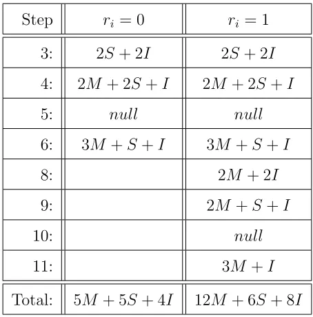
6.5 Complexity Analysis whenri = 0 . . . 58

6.6 Complexity Analysis whenri = 1 . . . 58

6.7 Comparison: the Number of Loops . . . 59

6.8 Computational Complexity Comparison . . . 59

(12)

LIST OF FIGURES

2.1 y2 ₌_x3₋₃_x_{+ 2 over}

R. [1] . . . 13

2.2 y2 ₌_x3 _over R. [1] . . . 13

2.3 y2 =x3+x+ 1 over _R. [1] . . . 13

2.4 y2 =x3−xover _R. [1] . . . 13

2.5 Elliptic Curve Points Addition. . . 14

2.6 Elliptic Curve Points Doubling. . . 15

3.1 The function (`P,Q) . . . 22

3.2 The function (`P,P) . . . 23

3.3 The function (νP+Q) . . . 23

4.1 A Function: (`[m]P,P/ν[m+1]P) . . . 29

4.2 Jump fromfm,P tof2m,P [1] . . . 31

6.1 Space-time Diagram of the Existing Works . . . 60

(13)

LIST OF ALGORITHMS

4.1 Miller’s Algorithm [2] . . . 32

5.1 Miller’s Algorithm Using Signed Digit Number [3] . . . 38

5.2 New Right-to-left Miller’s Algorithm . . . 44

(14)

LIST OF ACRONYMS

#E number of points on E

Fq finite field with prime numberq elements

Fqk full extension field

G a group of the bilinear map

D a divisor

Deg(D) the degree of a divisor D

e bilinear map

E(_Fq) elliptic curve over a finite field with prime number q elements

E(_Fqk) elliptic curve over a full extension field

r the largest prime order of a group inE(_Fq)

supp(D) the support of D

CPPA Conditional Privacy-preserving Authentication

DSRC Dedicated Short Range Communication

ECC Elliptic Curve Cryptosystem

(15)

1 INTRODUCTION

1.1 Pairing-based Cryptography and Its Applications

The Internet becomes increasingly important in our modern society. The Internet

technology has also progressed at a constant step to provide new and better services to

meet the demands from its users. Pairing-based cryptography (PBC) is an emerging

research area in the field of cryptography [4], which provides several new cryptographic

services over the Internet complement to conventional symmetrical and public key

cryptosystems. Some features and important facts about PBC include:

• PBC can provide several special security services, i.e., identity-based

encryp-tion, attribute-based encryption and anonymous authenticaencryp-tion, which are not

readily available from the conventional symmetrical and public key

cryptosys-tems.

• PBC studies mathematical bilinear function that can map a very complex

com-putational problem to a relatively simple one without compromising its security

strength.

• Pairing-based cryptography technology has been recently standardized in 2013

in P1363.3 “IEEE Standard for Identity-Based Cryptographic Techniques using

Pairings” [5].

Pairing-based cryptography can provide many unique or more efficient

cryptogra-phy and security services for the Internet, compared to conventional cryptographic

technology [6]. Its important applications are introduced as follows,

• Identity-based encryption [7]: in public key encryption system, the public key

of any user is based on his own identity. PBC is able to construct new

ID-based cryptographic primitives [8] to complement the conventional public key

(16)

• Key exchange: PBC can make a tripartite key exchange be done in one round

[9].

• Short signatures: Boneh-Lynn-Shacham (BLS) signature schemes [10] of PBC

only use a half of the length of other signature schemes [5].

• Anonymous authentication: the research work [11] has shown that

pairing-based cryptography can be applied to vehicular standard Dedicated Short Range

Communication (DSRC) [12]:

– DSRC is a communication service to distribute a message from a vehicle to all other vehicles or infrastructures to overcome the problem of the high

mobility environment [13] [14].

– The goals of DSRC are increasing road capacity [15], avoiding accidents, providing web or entertainment services. [16]

∗ The Conditional Privacy-preserving Authentication (CPPA) technique

[17] is one kind feasible scheme for DSRC, and it’s defined by the

fol-lowing algorithms: system setup, key generation, anonymous

authen-tication, and conditional tracking. These algorithms all use

pairing-based cryptography.

Bilinear map plays a central role in pairing-based cryptography. The popular

im-plementations of bilinear map are Weil pairing [18] and Tate pairing [19]. Miller’s

Algorithm [20], which is used to compute the Weil pairing and Tate pairing, is

prob-ably the most important and most computation-intensive algorithm in pairing-based

cryptography. This thesis proposes novel research works on improvement to Miller’s

(17)

1.2 Research Contribution

This thesis work concentrates on computational efficiency and security strength of

pairing-based cryptography. Since Miller’s Algorithm [20] is considered as the core

algorithm in pairing-based cryptography and most computational intensive, our

pro-posed work is aiming to improvement to Miller’s Algorithm [21] in terms of its

com-putational efficiency and resistance to side channel attacks. The proposed work can

be summarized as follows.

The original Miller’s Algorithm works in a manner of left to right. In this thesis

a right to left (R2L) version for Miller’s Algorithm is proposed. Moreover, the new

R2L algorithm has the feature of parallelism while the original version does not have.

When the algorithm is implemented in parallel architecture, it can be expected that

the proposed algorithm is much faster than the original Miller’s.

The second proposed work is a modified Miller’s Algorithm with enhanced security.

Compared to Miller’s Algorithm, the proposed algorithm not only makes parallel

computation possible but also has the nice property of resistance to certain side

channel attacks, i.e., simple power analysis.

The idea of using signed-digit binary number representation in Miller’s Algorithm

was first discussed in [3]. As an addition to the proposed works, an error in the

algorithm presented in [3] is found and corrected in this thesis.

1.3 The Scope and Organization of the Thesis

The organization of the rest of this thesis is as follows. In Chapter 2, mathematical

fundamentals which contain the modular operations, groups, finite fields and elliptic

curves over a finite field are introduced. In Chapter 3, the divisors and bilinear

map are explained, which provides important theoretical and algorithmic basis for

comprehending pairing-based cryptography. In Chapter 4 of the thesis, Weil pairing

(18)

are also reviewed and explained. The New Right-to-left Miller’s Algorithm and the

Modified Miller’s Algorithm with Enhanced Security are proposed in Chapter 5. In

Chapter 6, the complexities of the existing works and the proposed works are analyzed

and compared. It has been shown that the proposed algorithms have clear advantages

to the original Miller’s or its version using signed-digit binary number, in terms of

parallel-able computation and resistance to certain side channel attacks. Finally, the

(19)

2 MATHEMATICAL PRELIMINARIES

Finite field and elliptic curve are the cornerstones of pairing-based cryptography. In

this chapter, we introduce fundamental concepts, such like groups, finite fields and

their arithmetic, as well as elliptic curve defined over a finite field, and elliptic curve

point operations.

2.1 Modular Operations

2.1.1 Modular Operations (Integer)

1. x mod n means “the remainder of n dividing x” [22]. In other words, if x =

an+b, and a, b∈integer as well as 0≤b≤n−1, thenx modn =b.

2. Inverse: If ax= 1 mod n, then a is the inverse of x mod n [22]. There are two

popular methods to solve a:

• Method 1: Try every value fora < n until xa modn = 1.

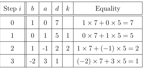
• Method 2: Euclidean method, which is usually used to solve the inverse of

big integers, so it is recommended to use Method 1 to solve the inverse of

small integers. No matter what usage Euclidean method is, Table 2.1 just

demonstrates how Euclidean method works with the 5a mod 7 = 1.

Table 2.1: Euclidean Method to Solve Inverse

Step i b a d k Equality

0 1 0 7 1×7 + 0×5 = 7

1 0 1 5 1 0×7 + 1×5 = 5

2 1 -1 2 2 1×7 + (−1)×5 = 2

3 -2 3 1 (−2)×7 + 3×5 = 1

(20)

– b0 = 1, a0 = 0, b1 = 0, and a1 = 1 are fixed, as well ask0 is null; – d0 = 7, d1 = 5 are given, then k1 is the quotient of d1 dividingd0; – b2 =b0−b1k1;

– a2 =a0−a1k1;

– d2 =d0−d1k1, d2 is also the remainder of d1 dividing d0; – k2 is the quotient of d2 dividingd1;

– Similarly, b3 = b1 −b2k2, a3 = a1 −a2k2, d3 = d1 −d2k2, k3 is the

quotient of d3 dividingd2;

...

bi =bi−2−bi−1ki−1,ai =ai−2−ai−1ki−1,di =di−2−di−1ki−1,ki is the

quotient of di dividingdi−1.

– Until di = 1 is gotten, stopping calculating and the value of ai is the final answer. Additionally, ki is unnecessary to be computed.

– In this instance, d3 = 1, so a3 = 3 is the answer.

2.1.2 Modular Operations (Polynomial)

1. Definition: f(x) mod P(x) means “the remainder of (f(x)÷P(x))” [22].

• It can be denotedf(x) =a(x)P(x)+b(x), where the degree ofb(x) is lower

than that of P(x), then f(x) mod P(x) = b(x).

• Polynomial division: (f(x)÷P(x)) to reap the remainder.

2. For example: x8 + 1 mod x3 +x2 + 1 = 6x2 −3x + 5, and the quotient is

(21)

2.2 Groups

2.2.1 Definition

A group is a setG together with a binary operation ∗ onG such that:

1. Binary operator ∗ is associative, i.e., for any a, b, c∈G,

a∗(b∗c) = (a∗b)∗c.

2. There exists an identity (or unity) element e∈G, i.e., for all a∈G,

a∗e=e∗a=a.

3. For each a∈G, there an inverse element a−1 _∈_G_{, such that}

a∗a−1 =a−1∗a=e.

2.2.2 Types of Groups

1. The operation ∗can be like ordinary multiplication or addition:

• Multiplicative group (and the unity is e= 1, if ∗ is multiplication.)

– Usually denoted by G×.

• Additive group (and the identity is e= 0, if ∗ is addition.)

– Usually denoted by G+_.

2. Infinite groups and finite groups

• Infinite group: there are infinite many elements in a group.

(22)

2.2.3 The Important Concepts of Groups

The computation details of the following concepts will be exemplified in “2.3

Back-ground Knowledge of Finite Field” . Hence, here just shows the outcomes.

1. A group Gis called cyclic group if there exists a group elementg such that any

other element in G can be written as gj _{for a certain integer} _{j >}_1.

• In this case, the group element g is called a generator of G, or a primitive

element inG.

• Example: G× = {1,2,3,4} under mod-5 multiplication is a cyclic group

with a primitive element 2. Because all the other group elements can be

written as a power of 2: G×={1,2,3,4}={24_,₂1_,₂3_,₂2_}_.

2. The order of group element a is defined as the minimal positive integer i such

that ai = the unity (or ai = 1 since the unity is 1 in this case). It is written

ord(a) =i. Clearly, a primitive element has the maximal order.

• In groupG× ={1,2,3,4}under mod-5 multiplication,ord(1) = 1; ord(2) =

4; ord(3) = 4; ord(4) = 2.

• G× ={1,2,3, ..., p−1}under mod-pmultiplication is a cyclic group, where

pis a prime.

– A primitive element in G× has the maximal order of p−1.

– Any other possible order of an element in this group has to be a factor of p−1.

(23)

2.3 Finite Fields

2.3.1 Definition

Finite field(or Galois field) is a set that has finitely many elements, and the result, which is operated by addition and multiplication of any two elements, is still closed

in the same set [22].

Note that the “closed” means the result, which is computed by any two elements,

still belongs to the same set, namely, the same finite field.

In other words to explain the definition, it is a set of finite many elements where

addition and multiplication are defined [23].

• The finite field is an additive group under the addition operation.

• All the nonzero elements in a finite field form a multiplicative group under

multiplication operation.

There are several popular families in finite fields, (_F is used to denote “Finite Field”), such as _Fq, F2k, _F₃k, and _F_qk [24]. Whereas, in this thesis, it just concerns

and discusses the _Fq and Fqk [25].

1. Finite field _Fq, where q is a prime number:

• The set is written as: _Fq ={0,1,2,3, ..., q−1}.

• The operations: modq addition, or mod q multiplication.

2. Finite field _Fqk, where q is a prime number, and k is an integer > 1:

• The set is written as: _Fqk ={polynomials of degree up to k−1 with

coef-ficients belonging to_Fq ={0,1,2,3, ..., q−1}, with irreducible polynomial f(x).}

• The operations: mod q polynomial addition; mod f(x) and mod q

(24)

2.3.2 The Arithmetic of Finite Field

It is an easy understanding way that demonstrates the arithmetic of finite field with

some examples of specific numbers operations.

1. Finite field _F5, and F5 ={0,1,2,3,4}:

• Mod q addition: a +b = (a +b) mod q. eg: (3 + 4) mod 5 = 2; (2 +

2) mod 5 = 4.

• Mod q multiplication: a ×b = (a×b) mod q. eg: (3×3) mod 5 = 4;

(2×4) mod 5 = 3.

2. Finite field _F22, and _F₂2 = {0,1, x, x+ 1} with irreducible polynomial f(x) = x2+x+ 1:

• Irreducible polynomials:

– Irreducible polynomial is similar to prime number for integers, an ir-reducible polynomial of degree n does not have a factor polynomial of

degree between 1 and n−1.

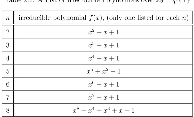
– Table 2.2 is a list of irreducible polynomials over _Z2 ={0,1}.

Table 2.2: A List of Irreducible Polynomials over_Z2 ={0,1}

n irreducible polynomial f(x), (only one listed for eachn)

2 x2+x+ 1

3 x3+x+ 1

4 x4+x+ 1

5 x5₊_x2_{+ 1}

6 x6₊_x_{+ 1}

7 x7₊_x_{+ 1}

(25)

• Addition: a+b = (a+b) mod 2. For example,

– (x+ (x+ 1)) mod 2 = (2x+ 1) mod 2 = 1

– (1 + (x+ 1)) mod 2 = (x+ 2) mod 2 =x

• Multiplication: a×b= (a×b) mod f(x) mod 2. For example,

– (x×(x+ 1)) mod f(x) mod 2 = (x2₊_x_{) mod (}_x2₊_x_{+ 1) mod 2 = 1} – ((x+ 1)×(x+ 1)) mod f(x) mod 2 = (x2 + 2x+ 1) mod (x2+x+

1) mod 2 = x

3. Another representation_F₂2, and_F₂2 ={0x+0,0x+1, x+0, x+1}={00,01,10,11}: the operations of addition and multiplication are similar to the previous

repre-sentation.

2.3.3 The Order of a Finite Field Element

1. For any a 6= 0 and a ∈ _Fq, the minimal positive integer j for aj = 1 is called the order of a, denoted by ord(a).

2. ai _with_i_{= 1}_,₂_{, ..., j}₋_{1 will be calculated. Till}_ai _{= 1, then}_i_{is called the order}

of a.

• Example: Find the order of all the nonzero elements in _F7. Solution:

ord(1) = 1, ord(2) = 3, ord(3) = 6,ord(4) = 3, ord(5) = 6,ord(6) = 2.

(26)

2.4 Elliptic Curve over a Finite Field

2.4.1 Definition

1. General Weierstrass equation for elliptic curves [1]:

E : y2+a1xy+a3y=x3+a2x2+a4x+a6 (1)

where a1, ..., a6 ∈F, this equation is usually used in F2k or _F₃k.

2. An elliptic curve E over a finite field is defined by

E : y2 =x3+ax+b where a, b∈_F (2)

• Basically, Equation (2) is called the short Weierstrass equation for elliptic

curves, in _Fq , Fqk and q6= 2 or 3.

• The thesis will always work on large prime fields, where the short

Weier-strass equation can cover all possible elliptic curves; thus, it will always be

used.

• The thesis only concentrates on an elliptic curve over finite fields. A finite

field has only finite many elements and a “curve defined over it should

have only finite many points.

3. What does an elliptic curve look like?

Usually, if elliptic curves are defined over finite field, they look like discrete

points sets; hence, the graphs with elliptic curves are demonstrated over _R so that they look like more smoothly.

(27)

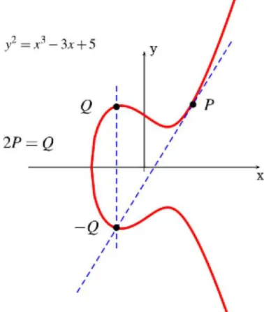
Fig. 2.1: y2 =x3−3x+ 2

over _R. [1] Fig. 2.2: y

2 ₌_x3 _over

R.

[1]

Fig. 2.3: y2 =x3+x+ 1

over _R. [1] Fig. 2.4: y2 ₌_x3₋_x_over

R. [1]

2.4.2 Elliptic Curve Points Operation

A point P(x0, y0) on elliptic curve E means: its coordinates x0 and y0 are elements

in the field, and the coordinates x0 and y0 satisfy Equation (2) [26].

1. Elliptic curve points addition:

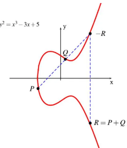
LetP, Qand Rbe three points on an elliptic curve. Points additionP +Q=R

(28)

Fig. 2.5: Elliptic Curve Points Addition.

Description: connect P and Q, then extend straight line `P,Q, it will intersect

elliptic curve on another point which is called point −R, and then mirror point

−R based on x-axis, pointR =P +Q is obtained.

2. Elliptic curve points doubling:

Let P, Qbe two points on an elliptic curve. Points doubling P +P = 2P =Q

(29)

Fig. 2.6: Elliptic Curve Points Doubling.

Description: pointP is the tangent point of straight line`P,P and elliptic curve,

then extend`P,P, it will intersect elliptic curve on another point which is called

point−Q, and then mirror point−Qbased onx-axis, pointQ= 2P is obtained.

2.4.3 Elliptic Curve Points Arithmetic

1. Let P1(x1, y1) and P2(x2, y2) be two points on the curve E : y2 =x3+ax+b,

where a, b∈_F [27].

• Assume P3(x3, y3) = P1(x1, y1) +P2(x2, y2)6=O, then

  

 

x3 =λ2−x1−x2

y3 =λ(x1−x3)−y1

where

λ

=

y2−y1

x₂−x₁ , if P1 6=P2; and

λ

=

3x2₁+a

2y₁ , if P1 =P2.

• For any elliptic curve, there exists the point at infinity O, defined by

P +O =P, or P + (−P) =P −P =O, for any point P ∈E.

(30)

– If y1 = 0 , then 2P1 =O.

– If P1 = (x1, y1)∈E, then −P1 = (x1,−y1)∈E.

2. Scalar multiplication [28]:

• LetP be a point on curveE defined in equation (2)

• Scalar multiplication nP is defined as

nP =P +P +P +...+P

| {z }

ntimes

where n is an integer; nP is also a point on the same curve E.

• The minimal positive integera for aP =O is called the order of P.

• Scalar multiplication is extensively required in elliptic curve cryptosystems.

2.4.4 The Structure for Points on Elliptic Curve

LetE(_Fq) denote the set of points on elliptic curve E defined over Fq.

1. Number of points on a curve E (the Hasse bound) [29]:

#E(_Fq) = q+ 1−t, |t|62

√

q. (3)

Note thatt is called the trace of Frobenius. It has been shown whenqis prime,

then every value N ∈[q+ 1−2√q, q+ 1 + 2√q] can be found as a group order

#E(_Fq) for some E.

2. E(_Fq) can be extended toE(Fqk) :kis the embedding degree is actually a

(31)

3. The Frobenius endomorphism π is defined as a map from E to E [31]

π: (x, y)7→(xq, yq) (4)

The Frobenius endomorphism maps any point inE(_Fq) to a point inE(Fq), but the set of points fixed by π is the group E(_Fq). As a result, π only does non-trivially on points in E(_Fq)\E(Fq), and more general representation is written as,

πi : (x, y)7→(xqi, yqi) (5)

acts non-trivially on points in E(_Fq)\E(Fqi).

Note that, E(_Fq) is a large set, which can be called E(Fqk) where k is the

embedding degree. Namely, E(_Fq) ⊂ E(Fq2) ⊂ E(_F_q3) ⊂, ..., ⊂ E(_F_qk−1) ⊂ E(_Fqk):

• E(_Fq)\E(Fq) means the set E(Fq) only excludes E(Fq).

• Likewise, E(_Fq)\E(Fqi) means the set E(_F_q) just excludes E(_F_qi), where

1< i < k.

2.4.5 Basics on Analytic Geometry

Let elliptic curve E be given as

E : y2 =x3+ax+b

And also let P = (x1, y1) and Q= (x2, y2) be two points on E.

(32)

solved as

k= y2−y1 x2−x1

and

d=y1−kx1 =

x2y1−x1y2 x2−x1

So it follows

`P,Q : y=

y2−y1 x2−x1

·x+x2y1−x1y2 x2−x1

(6)

Since in Chapter 4, Chapter 5 and Chapter 6, the Miller’s Algorithm with the

straight lines will be calculated, which includes the parameters of coordinates

x and y; consequently, Equation (6) can be written as

`P,Q: y−

y2−y1 x2−x1

·x−x2y1−x1y2 x2−x1

(7)

2. Let the tangent line `P,P toE at point P be given as y=k0x+d0. Thenk0 can

be solved as follows:

First find derivative ofE at point P:

(y2)0_x = (x3+ax+b)0_x

2yy_x0 = 3x2+a

It follows

k0 =y0_x|P =

3x2₊_a

2y

(x,y)=(x1,y1) = 3x

2 1 +a

2y1

then

d0 =y1−k0x1 =y1−

3x2 1+a

2y1

·x1 =

2y2

1 −3x31 −ax1

2y1

= −y

2

1+ 2ax1+ 3b

2y1

Hence,

(33)

Similarly, Equation (8) has the other representation,

`P,P : y− 3x2

1 +a

2y1

·x− −y 2

1 + 2ax1+ 3b

2y1

(9)

3. The vertical line νQ at point Q can be given as

νQ : x=x2 (10)

For the same reason, Equation (10) can be represented as

νQ : x−x2 (11)

The straight lines`P,Q,`P,P and νQare represented by Equation (7), (9) and (11),

re-spectively; so that they are conveniently substituted in the algorithms of the following

(34)

3 DIVISORS AND BILINEAR MAP

3.1 Divisors

Basically, divisors have wide definitions in algebraic geometry field, but this thesis

just concentrates on the parts which are used in the understanding of cryptographic

pairing computations [32].

3.1.1 Definition

A divisor D on curve E is a convenient way to denote a multi-set of points on E,

written as the formal sum [1]

D= X

P∈E( ¯Fq)

nP(P), wherenP ∈Z.

• The set of all divisors on E is denoted by Div

Fq(E) and forms a group, where

addition of divisors is natural.

• The zero divisor: it is the divisor with allnP = 0, the zero divisor 0∈Div_Fq(E).

• If the field _Fq is not specific, it can be omitted and simply written as Div(E) to denote the group of divisors.

A divisor D on curve E denotes the multiplicities of points on E; in other words,

it can represent a kind of relationship of lines and elliptic curve; moreover, it is the

cornerstone of pairing-based algorithms.

3.1.2 The Degree and Support of D

1. The degree of a divisor D is Deg(D) = P

(35)

2. The support of D, denoted by the set

supp(D) ={P ∈E(_Fq) :nP 6= 0}.

For instance,

Let P, Q, R, S ∈ E(_Fq). Let D1 = 3(P)−4(Q), and D2 = 4(Q) + (R)−2(S), so

the Deg(D1) = 3−4 = −1, and Deg(D2) = 4 + 1−2 = 3. The sum D1 +D2 =

3(P) + (R)−2(S), and naturally Deg(D1+D2) =Deg(D1) +Deg(D2) = 2.

The supports aresupp(D1) ={P, Q}, supp(D2) ={Q, R, S}, andsupp(D1+D2) =

{P, R, S}.

3.1.3 The Divisor of a Function f on E

1. The divisor of a function f on E is used to denote the intersection points (and

their multiplicities) of f and E.

• Let ordP(f) count the multiplicity of f atP, which is positive if f has a

zero at P, and negative if f has a pole at P. The divisor of a function f

is defined as

(f) = X P∈E(Fq)

ordP(f)(P).

• Notice that in all cases, Deg((`)) = 0. In fact, this is true for any function

f onE.

2. The relationship of a function f and a divisorD:

A divisor D=P

PnP(P) is a divisor of a function if and only if

X

P

nP = 0 and

X

P

[nP]P =O on E.

(36)

Let f be a line that intersects E at P and Q. Then divisor (f) = (`P,Q) =

(P) + (Q) + ([−1](P +Q))−3(O), since

X

P

nP =nP +nQ+n[−1](P+Q)+nO = 1 + 1 + 1−3 = 0

X

P

[nP]P =P +Q+ ([−1](P +Q)) =O (Elliptic Curve Points Operation)

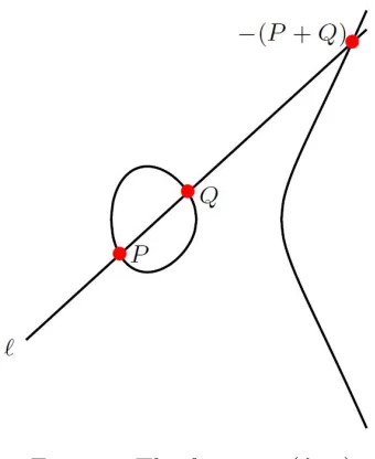
3. There are three scenarios that straight line f intersects curveE.

(a) In Fig. 3.1, the chord line `P,Q intersects E in P, Q and [−1](P +Q), all

with multiplicity 1, and `P,Q also intersects E with multiplicity−3 at O,

namely,`P,Q has a pole of order 3 atO. Thus, `P,Q has divisor

(`P,Q) = (P) + (Q) + ([−1](P +Q))−3(O). (12)

Fig. 3.1: The function (`P,Q)

(b) In Fig. 3.2, the tangent line`P,P intersectsEwith multiplicity 2 atP, with

(37)

case

(`P,P) = 2(P) + ([−2]P)−3(O). (13)

Fig. 3.2: The function (`P,P)

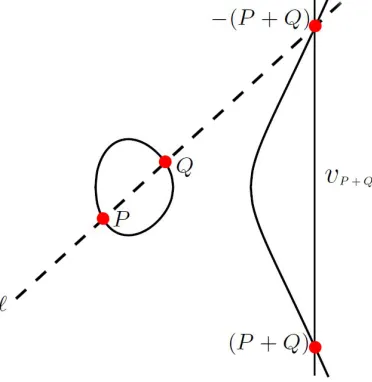
(c) In Fig. 3.3, the vertical line νP+Q intersectsE in (P+Q) and [−1](P +Q)

with multiplicity 1.

(νP+Q) = ((P +Q)) + ([−1](P +Q))−2(O). (14)

(38)

4. Properties of divisors of the functions:

(a) (f g) = (f) + (g)

(b) (f /g) = (f)−(g)

(c) (f) = 0 if and only if f is constant.

(d) If (f) = (g), then (f /g) = 0, sof is a constant multiple ofg.

3.1.4 Equivalence of Divisors

The divisorsD1 andD2 can be called equivalent, written as D1 ∼D2, D1 =D2+ (f)

for some function f. The notion of equivalence allows us to reduce divisors of any

size D into much smaller divisors.

For instance,

• LetR=P+QonE, so the line`joiningP andQhave divisor (`) = (P)+(Q)+

(−R)−3(O), whilst the vertical lineν=x−xR has divisor (ν) = (−R) + (R)−

2(O). In addition, the quotient `/ν has divisor (_ν`) = (P) + (Q)−(R)−(O).

Thus, the equationR =P+QonEis the same as the divisor equality (R)−(O)

= (P)−(O) + (Q)−(O)−(_ν`). It reduces (P) + (Q)−2(O) to (R)−(O)

• Similarly, in order to obtain ([2]Q)−(Q) = (Q)−(O), there exists a (f) = 2(Q)−

([2]Q)−(O). This equivalence will be used in following chapters’ algorithms to

substitute DQ = (Q)−(O) withDQ = ([2]Q)−(Q), so that it is convenient to

(39)

3.2 Bilinear Map

3.2.1 Definition

In pairing-based cryptography, bilinear map [33] plays a central role, it maps elements

of two cryptographic groups to a third group, in many literatures, it is written as

e:_G1×G2 →GT

Usually, bilinear map defines the groups _G1 inE(Fq),G2 inE(Fqk)/E(F_q), as well as

the target group _GT in the multiplicative group F∗_qk, so it can be called G1 and G2

are additive, whilst _GT is multiplicative [34].

If pointsP and Qare the elements of_G1 and G2, respectively. Then bilinear map

can be rewritten as

e(P, Q) :_G1×G2 →GT

where P ∈_G1 =E(Fq),Q∈G2 =E(Fqk)/E(_F_q), ande(P, Q)∈_G_T =_F∗ qk.

3.2.2 Properties

In many literatures, the properties of bilinear map are mentioned as,

• ForP, P0 ∈_G1 and Q, Q0 ∈G2,

e(P +P0, Q) = e(P, Q)·e(P0, Q),

e(P, Q+Q0) = e(P, Q)·e(P, Q0).

• For scalars a, b∈_Z,

e(P,0) =e(0, Q) = 1,

(40)

e([a]P, Q) =e(P, Q)a =e(P,[a]Q),

e([a]P,[b]Q) =e(P,[b]Q)a =e([a]P, Q)b =e(P, Q)ab =e([b]P,[a]Q).

3.2.3 Solve the Decision Diffie-Hellman (DDH) Problem with the Prop-erties

Bilinear map was initially found as an useful tool in cryptanalysis [35]; for instance,

it can solve the Decision Diffie-Hellman (DDH) Problem [36] [37]. In other words,

bilinear map can reduce the discrete logarithm problem on elliptic curves or

hyper-elliptic curves [18].

The Decision Diffie-Hellman (DDH) problem is: Given P,[a]P, b[P],andQ,

deter-mine whether Q= [ab]P or not [37].

Pairings make the DDH problem “easy”:

1) Computee(P, Q) =A,

2) Computee([a]P,[b]P) =B,

3) Q= [ab]P if and only if A=B.

Because e([a]P,[b]P) = e(P, P)ab ₌ _e₍_P,_[_ab_]_P_{), if} _e₍_P,_[_ab_]_P_{) =} _e₍_{P, Q}_{), then} _Q ₌

[ab]P.

3.2.4 Implementation Methods of e(P, Q)

There are two popular methods to implement e(P, Q):

• Weil pairingwr(P, Q)

• Tate pairing tr(P, Q) [38]

In this thesis, it concentrates on Weil pairing wr(P, Q) to implement bilinear map.

(41)

4 AN OVERVIEW OF MILLER’S ALGORITHM

AND RELATED WORKS

4.1 Weil Pairing

The Weil pairing (over finite fields):

LetP, Q∈E(_F_qk)[r] and letD_P andD_Qbedegree zero divisors withdisjoint supports

such thatDP ∼(P)−(O) and DQ∼(Q)−(O). There exist functions f and g such

that (f) = rDP and (g) = rDQ.

wr is a map:

wr :E(Fqk)[r]×E(_F_qk)[r]7→_F_qk[r],

defined as:

wr(P, Q) =

f(DQ) g(DP)

(15)

• Note thatr is the largest prime factor of #E(_Fq).

• For a pointP ∈E(_F_qk)[r], the functionf =f_r,P with divisorr(P)−r(O) plays

the major role in the Weil pairing definition.

• Likewise, for a point Q ∈ E(_Fqk)[r], the function g = g_r,Q has the divisor

r(Q)−r(O).

• According to Equation (15), wr(P, Q) equals to f(DQ) divides g(DP).

More-over,f(DQ) andg(DP) can be calculated with Miller’s Algorithm, respectively.

Consequently, this chapter just performs how calculates f(DQ) using Miller’s

Algorithm; on the other hand, under the Miller’s Algorithm,g(DP) can use the

(42)

4.2 Miller’s Algorithm

In this section, it is necessary to recall the knowledge of divisors and the function f.

Some important equations will be deducted:

• For any m ∈ _Z and P ∈ E, it follows that there exists a function fm,P with

divisor

(fm,P) = m(P)−([m]P)−(m−1)(O), (16)

– where it is noted that for m= 0, it can take f0,P = 1 with (f0,P) the zero divisor.

(f0,P) = 0(P)−([0]P)−(0−1)(O) = 0,

– where it is noted that for m= 1, it can take f1,P = 1 with (f1,P) the zero divisor.

(f1,P) = 1(P)−([1]P)−(1−1)(O) = 0,

– Note: (f0,P) = (f1,P) = zero divisor, according to “Properties of divisors of functions: (f) = 0 if and only if f is constant”, so it is convenient to

take f0,P =f1,P = 1 for setting the initial value.

• From fm,P tofm+1,P:

– When P ∈ E[r], means r is the order of P, then following (16), fr,P has divisor

(fr,P) =r(P)−r(O). (17)

Furthermore,

(43)

Observe that, Equation (18) subtracts Equation (16), then acquire

(fm+1,P)−(fm,P) = (P) + ([m]P)−([m+ 1]P)−(O). (19)

– In Fig. 4.1, according to the functions of chord line and vertical line, it is obtained

(`[m]P,P) = (P) + ([m]P) + (−[m+ 1]P)−3(O),

(ν[m+1]P) = (−[m+ 1]P) + ([m+ 1]P)−2(O),

Thus,

(`[m]P,P/ν[m+1]P) = (`[m]P,P)−(ν[m+1]P) = (P) + ([m]P)−([m+ 1]P)−(O)

(20)

where`[m]P,P andν[m+1]P are the chord and vertical lines used in the

chord-and-tangent addition of the point [m]P and P.

(44)

From (19) and (20) it can be seen that (fm+1,P)−(fm,P) is exactly the

divisor of the function `[m]P,P/ν[m+1]P, which means fm+1,P can be built

fromfm,P via

fm+1,P =fm,P ×

`[m]P,P ν[m+1]P

(21)

• From fm,P tof2m,P:

– In addition, according to Properties “ (f g) = (f) + (g) ”:

(f_m,P2 ) = (fm,P ×fm,P) = (fm,P) + (fm,P) = 2(fm,P),

Hence, following (16)

(f_m,P2 ) = 2(fm,P) = 2m(P)−2([m]P)−2(m−1)(O);

Moreover, also following (16)

(f2m,P) = 2m(P)−([2m]P)−(2m−1)(O),

Observe that,

(f2m,P)−(fm,P2 ) = 2([m]P)−([2m]P)−(O).

– Now, the functions of chord line and vertical line can be rewritten as:

(`[m]P,[m]P) = ([m]P) + ([m]P) + (−[2m]P)−3(O),

(45)

Similarly, according to (20), it is obtained

(`[m]P,[m]P/ν[2m]P) = (`[m]P,[m]P)−(ν[2m]P) = 2([m]P)−([2m]P)−(O),

Therefore,

(f2m,P)−(fm,P2 ) = 2([m]P)−([2m]P)−(O) = (`[m]P,[m]P/ν[2m]P)

At last,

f2m,P =fm,P2 ×

`[m]P,[m]P ν[2m]P

(22)

– Based on (22), it can be straightly jumped fromfm,P tof2m,P, in compar-ison with the naive method of progressing one-by-one in Fig. 4.2:

Fig. 4.2: Jump from fm,P tof2m,P [1]

So far, for any m, either fm+1,P, or f2m,P can be obtained quickly, Miller

observed that, then gives rise to a double-and-add style algorithm.

1. This is the Miller’s Algorithm, then an example will be given to demonstrate

(46)

Algorithm 4.1 Miller’s Algorithm [2]

Input: P ∈ E(_F_qk)[r], D_Q ∼ (Q)−(O) with support disjoint from (f_r,P), and r =

(rn−1...r1r0)2 with rn−1 = 1. Output: fr,P(DQ)←f.

1: R←P, f ←1.

2: for i=n−2 down to 0 do

3: Compute the line function `R,R.

4: R ←[2]R.

5: Compute the line function νR.

6: f ←f2 ×`R,R νR (DQ).

7: if ri = 1, then

8: Compute the line function `R,P.

9: R←R+P.

11: f ←f × `R,P νR (DQ).

12: end if

13: end for

14: return f.

• Steps 3-6 of Algorithm 4.1 can be called a doubling stage, which is different from elliptic curve points’ doubling operation.

• Steps 7-12 of Algorithm 4.1 can be called an addition stage, which is different from elliptic curve points’ addition operation.

• The algorithm calculates r from the most significant digit to the least

significant digit (where r is a binary number of length n), namely, the

sequence of computation is from left to right.

2. The details of the computation:

Input: P, DQ, r= 29 = (11101)2 Output: f29,P(DQ)←f

Compute:

(47)

i. `P,P

ii. 2P = 2×P

iii. ν2P

iv. f2,P =f12,P × `P,P

ν2P (DQ)

v. `2P,P

vi. 3P = 2P +P

vii. ν3P

viii. f3,P =f2,P × `2P,P

ν3P (DQ)

(c) r2 = 1:

i. `3P,3P

ii. 6P = 2×3P

iii. ν6P

iv. f6,P =f32,P × `3P,3P

ν6P (DQ)

v. `6P,P

vi. 7P = 6P +P

vii. ν7P

viii. f7,P =f6,P × `6P,P

ν7P (DQ)

(d) r1 = 0:

i. `7P,7P

ii. 14P = 2×7P

iii. ν14P

iv. f14,P =f72,P × `7P,7P

ν14P (DQ)

(e) r0 = 1:

i. `14P,14P

(48)

iii. ν28P

iv. f28,P =f142,P × `14P,14P

ν28P (DQ)

v. `28P,P

vi. 29P = 28P +P

vii. ν29P

viii. f29,P =f28,P × `28P,P

ν29P (DQ)

(f) return f29,P

• Note:

– The steps v to viii of (e) need to be noticed, becauser = 29 is the order of point P, that means 29P = O. As a result, O = 29P = 28P +P,

namely, 28P =−P.

– As a consequence, in step v of (e), it can be written `28P,P = `−P,P. Based on the geometry, the chord line `−P,P is just the vertical line

νP. Fortunately, it just conveniently computes νP instead of `28P,P in

step v of (e).

– In step vi of (e), O = 29P = 28P +P; thus, this step doesn’t need to be computed.

– In projective plane, O is defined as O = (0 : 1 : 0), and

νO : y= 1,

in step vii of (e), ν29P =νO, so ν29P equals to constant 1.

– Finally, in step viii of (e),

f29,P =f28,P × `28P,P

ν29P

(DQ) =f28,P × νP

(49)

In generalization, when computes the last loop of Miller’s Algorithm, it is

able to use

νP instead of`[r−1]P,P

and

constant 1 instead of ν[r]P

to simplify the last several steps.

Hence, the last step can be written as:

fr,P =fr−1,P ×

`[r−1]P,P ν[r]P

(DQ) = fr−1,P × νP

1 (DQ) = fr−1,P ×νP(DQ)

Additionally,O =rP doesn’t have to be computed.

3. Now, it is time to explain how to compute _ν`(DQ):

(a) DQ ∼ (Q)−(O), based on the concept of “Equivalence of Divisors” in

the Subsection (3.1.4) at the Page 24, ([2]Q)−(Q)∼(Q)−(O), so

equa-tion DQ = ([2]Q)−(Q) can be obtained. Although using this equivalence

“DQ = ([2]Q)−(Q)”, it still follows the input restriction of Miller’s

Algo-rithm (P and DQ with support disjoint from (fr,P)).

(b) Functions` and ν can be calculated respectively, according to the

Subsec-tion (2.4.5) at the Page 17.

(c) Under the divisor theory:

`

ν(DQ) =

`(DQ) ν(DQ)

= `(([2]Q)−(Q)) ν(([2]Q)−(Q))

moreover,

`(([2]Q)−(Q)) = `([2]Q)

`(Q) ; ν(([2]Q)−(Q)) =

(50)

Thus,

`

ν(DQ) =

`([2]Q) `(Q) ×

ν(Q) ν([2]Q) =

`([2]Q)×ν(Q)

`(Q)×ν([2]Q) (23)

(d) At last, correspondingly substituting the x-coordinates and y-coordinates

of point [2]Q and pointQinto the functions `and ν in Equation (23), the

result of _ν`(DQ) can be gotten.

Therefore, these steps are the details of calculating _ν`(DQ).

4. There is another existing work, Miller’s Algorithm Using Signed Digit Number

[3]. However, its one problem makes it cannot work, and the problem will be

(51)

5 PROPOSED WORKS

In this chapter, the correction of existing work “Miller’s Algorithm Using Signed Digit

Number” will be attested. Moreover, two new algorithms will be proposed: the New

Right-to-left Miller’s Algorithm and the Modified Miller’s Algorithm with Enhanced

Security. These two algorithms have different features and usages. In addition, their

examples and contributions will also be demonstrated.

5.1 The Correction of Miller’s Algorithm Using Signed Digit

Number

In every loop of Miller’s Algorithm, if ri = 0, then it just needs a doubling stage

(steps 3-6 of Algorithm 4.1); whilst, if ri = 1, then it needs a doubling stage plus

an addition stage (steps 7-12 of Algorithm 4.1), that means the total steps are steps

3-12 of Algorithm 4.1. Consequently, whenri = 1, the Algorithm needs around twice

computation steps in comparison with ri = 0 [39].

Hence, when the length of r = (rn−1...r1r0)2 is not changed, increasing the the

number of zero and decreasing the the number of nonzero, it is able to keep the number

of the doubling stages unchanged and lessen the number of the addition stages [40];

as a result, calculation will be more efficient [41].

For this motivation, Miller’s Algorithm Using Signed Digit Number substitutes

binary number system with signed digit number system, and the signed digit number

system can increase the number of zero and reduce the the number of nonzero, so it is

able to decrease the calculation steps relatively, such that it can make the computation

more efficient [42].

(52)

Algorithm 5.1 Miller’s Algorithm Using Signed Digit Number [3]

Input: P ∈ E(_F_qk)[r], D_Q ∼ (Q)−(O) with support disjoint from (f_r,P), and r =

(rn−1...r1r0)2 with rn−1 = 1.Additionally, ri ∈ {1,0,1}.

Output: fr,P(DQ)←f.

1: R←P, f ←1.

3: Compute the line function `R,R.

4: R ←[2]R.

6: f ←f2 ×`R,R νR (DQ).

7: if ri = 1, then

9: R←R+P.

11: f ←f × `R,P νR (DQ).

12: end if

13: if ri = 1, then

15: R←R−P.

16: Compute the line function `−R,P *

17: f ←f × νR

`−R,P(DQ). *

18: end if

19: end for

20: return f.

* These two steps of this algorithm [3] are wrong when ri = 1, it will be corrected

when calculating the step of ri = 1.

Likewise, the algorithm calculates r from the most significant digit to the least

significant digit (where r is a binary number of length n), namely, the sequence of

computation is also from left to right.

1. Correct the Miller’s Algorithm Using Signed Digit Number

When ri = 1, namely, it needs to be calculated the function from fm+1,P to

fm,P:

Based on (21),

(53)

Acquire that,

fm,P =fm+1,P ×

ν[m+1]P `[m]P,P

(24)

Therefore, when ri = 1, the corrected steps 16 and 17 should be

17: f ←f× νR

`R,P(DQ).

2. It will be exemplified the correction is accurate, but the two significant steps of

the original Miller’s Algorithm Using Signed Digit Number are wrong.

• This computation follows the correction:

Compute:

(a) P; f1,P = 1,

(b) r4 = 0:

i. `P,P

ii. 2P = 2×P

iii. ν2P

iv. f2,P =f12,P × `P,P

ν2P (DQ)

(c) r3 = 0:

i. `2P,2P

ii. 4P = 2×2P

iii. ν4P

iv. f4,P =f22,P × `2P,2P

(54)

(d) r2 = 1: these steps of (d) are different from the original Miller’s

Al-gorithm.

i. `4P,4P

ii. 8P = 2×4P

iii. ν8P

iv. f8,P =f42,P × `4P,4P

ν8P (DQ)

v. ν8P

vi. 7P = 8P −P

vii. `7P,P

viii. f7,P =f8,P × _`ν8P 7P,P(DQ)

(e) r1 = 0:

i. `7P,7P

ii. 14P = 2×7P

iii. ν14P

iv. f14,P =f72,P × `7P,7P

ν14P (DQ)

(f) r0 = 1:

i. `14P,14P

ii. 28P = 2×14P

iii. ν28P

iv. f28,P =f142,P × `14P,14P

ν28P (DQ)

v. `28P,P

vi. 29P = 28P +P

vii. ν29P

viii. f29,P =f28,P × `28P,P

(55)

The last steps v to viii of (f) are also able to follow the Note in the

Sub-section (4.2) at the Page 34 to calculate.

Thus, following the correction can smoothly obtain the final result.

• If the computations follow theMiller’s Algorithm Using Signed Digit

Num-ber, then the steps in (d) of the correction will be:

(d) r2 = 1:

i. `4P,4P

ii. 8P = 2×4P

iii. ν8P

iv. f8,P =f42,P × `4P,4P

ν8P (DQ)

v. ν8P

vi. 7P = 8P −P

vii. `−7P,P *

viii. f7,P =f8,P × _`₋ν8P

7P,P(DQ) *

There are two important aspects that incur the inaccuracy of theMiller’s

Algorithm Using Signed Digit Number:

– r = 29 is the order of point P, that means O = 29P = 22P + 7P, namely, 22P = −7P. In this way, `−7P,P could be `22P,P in step vii.

On the other hand, when it calculates the point 7P, it cannot jump to

reckon the point 22P because both Elliptic Curve points operation and

Miller’s Algorithm are accumulative computations. What is more, if

calculating`−7P,P in step vii, then the step vi (7P = 8P−P) is useless.

Therefore, in this circumstance, reckoning `−7P,P is neither accurate

(56)

– According to Equation (24)

fm,P =fm+1,P ×

ν[m+1]P `[m]P,P

f7,P should equal to

f8,P × ν8P `7P,P

(DQ)

neither

f8,P × ν8P `−7P,P

(DQ)

nor

f8,P × ν8P `22P,P

(DQ)

f7,P cannot be gotten using the last two representations, so the

com-putation cannot proceed to go. In other words,

f7,P =f8,P × ν8P `7P,P

(DQ)

f7,P 6=f8,P × ν8P `−7P,P

(DQ)

f7,P 6=f8,P × ν8P `22P,P

(DQ)

finally, `−7P,P should be`7P,P.

Conclusively, the correction of Miller’s Algorithm Using Signed Digit Number

is accurate and works.

5.2 New Right-to-left Miller’s Algorithm

New Right-to-left Miller’s Algorithm will use two core equations:

(57)

and

fm+n,P =fm,P ×fn,P ×

`[m]P,[n]P ν[m+n]P

(26)

Equation (25) has been proved in the Subsection (4.2) from the Page 28 to the

Page 31. Observe that, Equation (26) just substitutes m in Equation (25) with n;

moreover, it will be attested in divisor level.

• From fm,P and fn,P to fm+n,P:

According to Equation (16),

(fm,P) = m(P)−([m]P)−(m−1)(O) (27)

substituting m with n and m+n, then

(fn,P) =n(P)−([n]P)−(n−1)(O) (28)

(fm+n,P) = (m+n)(P)−([m+n]P)−(m+n−1)(O) (29)

Moreover,

(`[m]P,[n]P) = ([m]P) + ([n]P) + (−[m+n]P)−3(O), (30)

(ν[m+n]P) = (−[m+n]P) + ([m+n]P)−2(O), (31)

Therefore, in divisor level

Equation(29) =Equation(27) +Equation(28) +Equation(30)−Equation(31)

Namely,

(58)

The New Right-to-left Miller’s Algorithm calculates r from the least significant

digit to the most significant digit (where r is a binary number of length n), in other

words, the computational sequence is from right to left, but the existing works are

on the contrary, so the proposal proposed a new option. On the other hand, it can

compute the fr,P(DQ) more efficiently, and it will be compared with the existing

works in Chapter 6.

Algorithm 5.2 New Right-to-left Miller’s Algorithm

Input: P ∈ E(_F_qk)[r], D_Q ∼ (Q) − (O) with support disjoint from (f_r,P), and

r= (rn−1...r1r0)2, and ri ∈ {0,1}.

Output: fr,P(DQ)←fα.

1: P1 ← O, fα ←f1,P = 1; P2 ←P, fβ ←f1,P = 1.

2: for i= 0 up to n−1 do

3: if ri = 1, then

4: Compute the line functions `P1,P2; `P2,P2.

5: P1 ←P1+P2; P2 ←[2]P2.

6: Compute the line functions νP1; νP2.

7: fα ←fα×fβ× `P₁,P₂

νP1

(DQ); fβ ←fβ2× `P₂,P₂

νP2

(DQ).

8: else

9: Compute the line function `P2,P2.

10: P2 ←[2]P2.

11: Compute the line function νP2.

12: fβ ←fβ2× `P₂,P₂

νP₂ (DQ).

13: end if

14: end for

15: return fα.

1. There is a little trick to deal with the last loop:

ri ∈ {0,1} means the first digit rn−1 must equal to 1; in addition, the final

return is fα rather than fβ. Therefore, when the Algorithm 5.2 computes the

last loop (rn−1 = 1), just doing the process to compute the value of fα is fine,

and it is unnecessary to do the process to compute the value of fβ.

(59)

the steps of computing thefα and removes the steps of computing thefβ:

when rn−1 = 1,

• Compute the line function `P1,P2.

• P1 ←P1+P2

• Compute the line function νP1.

• fα ←fα×fβ × `P1,P2

νP₁ (DQ).

Consequently, when it preforms the little trick, it is capable of saving the steps

of computing the fβ in the last loop.

2. An example of the New Right-to-left Miller’s Algorithm:

Compute:

(a) O, f1,P = 1; P, f1,P = 1.

(b) r0 = 1:

i. `O,P; `P,P

ii. P =O+P; 2P = 2×P

iii. νP; ν2P

iv. f1,P =f1,P ×f1,P × `O,P

νP (DQ) = 1; f2,P =f

2 1,P ×

`P,P ν2P (DQ)

(c) r1 = 0:

i. `2P,2P

ii. 4P = 2×2P

iii. ν4P

iv. f4,P =f22,P × `2P,2P

(60)

(d) r2 = 1:

i. `P,4P; `4P,4P

ii. 5P =P + 4P; 8P = 2×4P

iii. ν5P; ν8P

iv. f5,P =f1,P ×f4,P × `P,4P

ν5P (DQ); f8,P =f

2 4,P ×

`4P,4P ν8P (DQ)

(e) r3 = 0:

i. `8P,8P

ii. 16P = 2×8P

iii. ν16P

iv. f16,P =f82,P × `8P,8P

ν16P (DQ)

(f) r4 = 1:

i. `5P,16P; `16P,16P

ii. 21P = 5P + 16P; 32P = 2×16P

iii. ν21P; ν32P

iv. f21,P =f5,P ×f16,P × `5P,16P

ν21P (DQ); f32,P =f

2 16,P ×

`16P,16P ν32P (DQ)

(g) r5 = 1:

i. `21P,32P; `32P,32P

ii. 53P = 21P + 32P; 64P = 2×32P

iii. ν53P; ν64P

iv. f53,P =f21,P ×f32,P ×

`21P,32P

ν53P (DQ); f64,P =f

2 32,P ×

`32P,32P ν64P (DQ)

(h) return f53,P

Notice:

(61)

(νP) = (P) + (−P)−2(O)

obtain (`O,P

νP ) = (`O,P −νP) = zero divisor, it can be f1,P = 1.

Generally, the equation can be an universal equation,

(`O,[m]P ν[m]P

) = (`O,[m]P −ν[m]P) = zero divisor, it can be 1.

because of

(`O,[m]P) = ([m]P) + (O) + ([−m]P)−3(O)

(ν[m]P) = ([m]P) + ([−m]P)−2(O)

Namely, when the computation needs to calculate `O,[m]P and ν[m]P, it

does not have to calculate them, and can obtain the result of `O,[m]P ν[m]P = 1,

directly.

• In step (g), it can use the little trick which is mentioned at the Page 44, so

that it can save the computational steps off64,P. Thus, the step (g) could

be:

(g) r5 = 1:

i. `21P,32P

ii. 53P = 21P + 32P

iii. ν53P

iv. f53,P =f21,P ×f32,P ×

`21P,32P ν53P (DQ)

3. The contributions of the New Right-to-left Miller’s Algorithm:

(62)

• This is a new option for some particular designs.

• It can make cyber attackers confused: even if they obtain every digits

ofr, they may not guess the sequence ofrwhich is not the conventional

sequence (from left to right).

Thus, the new sequence (from right to left) may be securer.

(b) Whenri = 1, there is a semicolon (;) to separate two computations in every step, that means the separated computations are independent, and their

computations can start at the same time and not influence each other.

In other words, the separated computations by a semicolon are parallel

computation.

Hence, when ri = 1, the computational time is just the maximum of

dou-bling stage and addition stage. Nevertheless, the existing works are all

se-rial computation that the computational time is the sum of doubling stage

and addition stage. Therefore, the New Right-to-left Miller’s Algorithm

speeds up and is more efficient. There will be more detailed comparison

in next chapter.

5.3 Modified Miller’s Algorithm with Enhanced Security

The aim of the modified Miller’s Algorithm is against certain side channel attack

in pairing-based cryptography (PBC), so it has to assure the complexities of two

conditions (when ri = 1 and ri = 0) are the same, so that attackers cannot analyze

out which ri equals to 1 or 0. Thus, they are not able to obtain the final value of

r. In other words, the modified Miller’s Algorithm is secure in against certain side

channel attack, i.e., simple power analysis.

The followings are the modified algorithm and its instance; additionally, the

(63)

Algorithm 5.3 Modified Miller’s Algorithm with Enhanced Security

Input: P ∈ E(_F_qk)[r], D_Q ∼ (Q) − (O) with support disjoint from (f_r,P), and

r= (rn−1...r1r0)2 with rn−1 = 1, and ri ∈ {0,1}.

Output: fr,P(DQ)←fα.

1: P1 ←P, fα ←f1,P = 1; P2 ←[2]P, fβ ←f2,P = `P,P ν[2]P(DQ).

3: if ri = 1, then

5: P1 ←P1+P2; P2 ←[2]P2.

7: fα ←fα×fβ× `P₁,P₂

νP₁ (DQ); fβ ←f

2

β × `P₂,P₂

νP₂ (DQ).

8: else

10: P2 ←P1+P2; P1 ←[2]P1.

12: fβ ←fα×fβ × `P1,P2

νP₂ (DQ); fα ←f

2

α× `P1,P1

νP₁ (DQ).

13: end if

14: end for

15: return fα.

1. Algorithm 5.3 still use the following two core equations:

f2m,P =fm,P2 ×

`[m]P,[m]P ν[2m]P

and

`[m]P,[n]P ν[m+n]P

They were proved in previous sections, the first one has been proved in the

Subsection (4.2) from the Page 28 to the Page 31, and the second one has been

proved in the Subsection (5.2) from the Page 42 to the Page 44.

2. An example of the Modified Miller’s Algorithm with Enhanced Security:

(64)

(a) P, f1,P = 1; 2P, f2,P = `P,P ν[2]P(DQ).

(b) r4 = 1:

i. `P,2P; `2P,2P

ii. 3P =P + 2P; 4P = 2×2P

iii. ν3P; ν4P

iv. f3,P =f1,P ×f2,P × `P,2P

ν3P (DQ); f4,P =f

2 2,P ×

`2P,2P ν4P (DQ)

(c) r3 = 0:

i. `3P,4P; `3P,3P

ii. 7P = 3P + 4P; 6P = 2×3P

iii. ν7P; ν6P

iv. f7,P =f3,P ×f4,P × `3P,4P

ν7P (DQ); f6,P =f

2 3,P ×

`3P,3P ν6P (DQ)

(d) r2 = 1:

i. `7P,6P; `7P,7P

ii. 13P = 7P + 6P; 14P = 2×7P

iii. ν13P; ν14P

iv. f13,P =f7,P ×f6,P × `7P,6P

ν13P (DQ); f14,P =f

2 7,P ×

`7P,7P ν14P (DQ)

(e) r1 = 0:

i. `13P,14P; `13P,13P

ii. 27P = 13P + 14P; 26P = 2×13P

iii. ν27P; ν26P

iv. f27,P =f13,P ×f14,P ×

`13P,14P

ν27P (DQ); f26,P =f

2 13,P ×

`13P,13P ν26P (DQ)

(f) r0 = 1:

(65)

iii. ν53P; ν54P

iv. f53,P =f27,P ×f26,P ×

`27P,26P

ν53P (DQ); f54,P =f

2 27,P ×

`27P,27P ν54P (DQ)

(g) return f53,P

3. The contributions of the Modified Miller’s Algorithm with Enhanced Security:

(a) As aforementioned, it is against certain side channel attack, i.e., simple

power analysis because the computational complexities of two different

conditions are equal; namely, no matter whenri = 1 orri = 0, the

compu-tations are balance, so that the value ofr cannot be analyzed out. Thus,

this proposed algorithm can be against certain side channel attack.

(b) The computational efficiency are not reduced in comparison with the

ex-isting works, even more efficient because of the parallel computation.

In every loop, there is a semicolon (;) to separate two computations in every step, that means the separated computations are independent, and

their computations can start at the same time and not impact mutually.

In other words, the separated computations by a semicolon are parallel

computation.

Consequently, the computational time is just the maximum of doubling

stage and addition stage. However, the existing works are serial

compu-tation which the compucompu-tational time is the sum of doubling stage and

addition stage. Therefore, the Modified Miller’s Algorithm with Enhanced

Security is not only more efficient than the existing works but also has the

(66)

6 COMPLEXITY ANALYSIS AND

COMPARI-SON

In this chapter, the comparison amongst the two existing works and the two

pro-posed works will be demonstrated. Additionally, it will analyze the complexities in

computational cost level. Namely,

• M: represents the computational cost of a multiplication;

• S: represents the computational cost of a squaring;

• I: represents the computational cost of an inversion.

The analyses ignore the computational cost of addition (A) because it is trivial in

comparison with any of M, S andI. What’s more, the computational costI 20M

over _Fq and Fqk, and “the multiplication to inversion ratio is commonly reported to

be 80 : 1 or higher” [1].

6.1 Computational Complexity Analysis

6.1.1 Complexity Analysis of Points Operation over Elliptic Curve

In the Section (2.4.3) at the Page 15:

Let P1(x1, y1) and P2(x2, y2) be two points on the curve E : y2 = x3 +ax+b,

where a, b∈_F.

* Assume P3(x3, y3) =P1(x1, y1) +P2(x2, y2)6=O,then

  

 

x3 =λ2−x1−x2

y3 =λ(x1−x3)−y1

where

λ

=

y2−y1 , if P 6=P ; and

λ

=

3x

2 1+a

(67)

Observably,

• Points doubling costs: 2M + 2S+I

• Points addition costs: 2M +S+I

6.1.2 Complexity Analysis of Straight Lines

In the Section (2.4.5) at the Page 17:

Let elliptic curve E be given as E : y2 ₌_x3₊_ax₊_b_{, and also let} _P _{= (}_x 1, y1)

and Q= (x2, y2) be two points on E.

• Chord line,

`P,Q: y−

y2−y1 x2−x1

·x−x2y1−x1y2 x2−x1

• Tangent line,

`P,P : y− 3x2

1 +a

2y1

·x− −y 2

1 + 2ax1+ 3b

2y1

• Vertical line,

νQ : x−x2

Note:

It just considers the costs which are caused by x1, y1 and x2, y2, excluding the

unknown coordinatesx, y.

In the existing works and the proposed works, the steps of computing lines just

calculate out the line FUNCTIONS; namely, they obtain the representations of x, y,

andx, y do not need to be calculated. On the other hand, after it completes the steps

of computing lines, substituting the values of x, y into the line functions are other

steps, and at that time x just multiplies a constant. Therefore, the costs which are

caused by x, y are ignored.

(68)

• Chord line costs: 2M + 2I

• Tangent line costs: 2S+ 2I

• Vertical line costs: null

6.1.3 Complexity Analysis of _ν`(DQ)

In the point (3) of the Section (4.2) at the Page 35:

Based on

`

ν(DQ) =

`([2]Q) `(Q) ×

ν(Q) ν([2]Q) =

`([2]Q)×ν(Q) `(Q)×ν([2]Q)

It can be observed that both chord line and tangent line have the same cost: 2M+I.

6.1.4 Complexity Analysis of the Existing Works and the Proposed Works

In this subsection, it will analyze the complexity of each step when ri = 0, ri = 1,

and ri = 1, respectively. In addition, they are all based on each computable step of

every algorithm and the previous complexity analyses.

Efficient Computation of Miller's Algorithm in Pairing-Based Cryptography

Scholarship at UWindsor

Scholarship at UWindsor

Efficient Computation of Miller's Algorithm in Pairing-Based

Efficient Computation of Miller's Algorithm in Pairing-Based

Cryptography

Cryptography

Efficient Computation of Miller’s Algorithm in

Pairing-Based Cryptography

by

Shun Wang

A Thesis

Submitted to the Faculty of Graduate Studies

through Electrical and Computer Engineering

in Partial Fulfillment of the Requirements for

the Degree of Master of Applied Science at the

University of Windsor

Windsor, Ontario, Canada

2017

c

Efficient Computation of Miller’s Algorithm in Pairing-Based

Cryptography

AUTHOR’S DECLARATION OF ORIGINALITY

ABSTRACT

DEDICATION

ACKNOWLEDGMENTS

TABLE OF CONTENTS

LIST OF TABLES

LIST OF FIGURES

LIST OF ALGORITHMS

LIST OF ACRONYMS

1

INTRODUCTION

1.1

Pairing-based Cryptography and Its Applications

1.2

Research Contribution

1.3

The Scope and Organization of the Thesis

2

MATHEMATICAL PRELIMINARIES

2.1

Modular Operations

2.2

Groups

2.3

Finite Fields

2.4

Elliptic Curve over a Finite Field

λ

=

λ

=

3

DIVISORS AND BILINEAR MAP

3.1

Divisors

3.2

Bilinear Map

4

AN OVERVIEW OF MILLER’S ALGORITHM

AND RELATED WORKS

4.1

Weil Pairing

4.2

Miller’s Algorithm

5

PROPOSED WORKS

5.1

The Correction of Miller’s Algorithm Using Signed Digit

Number

5.2

New Right-to-left Miller’s Algorithm

5.3

Modified Miller’s Algorithm with Enhanced Security

6

COMPLEXITY ANALYSIS AND

COMPARI-SON

6.1

Computational Complexity Analysis