Electromagnetic Tethers as Deorbit Devices - Numerical Simulation of Upper-Stage Deorbit Efficiency

Electromagnetic Tethers as Deorbit Devices -

Numerical Simulation of Upper-Stage Deorbit

Efficiency

Alexandru Ionel

INCAS - National Institute for Aerospace Research “Elie Carafoli”, Bdul Iuliu Maniu 220, Bucharest

ABSTRACT: This paper examines the deorbit efficiency of an electromagnetic tether deorbit device when used to deorbit an upper stage at end of mission from low Earth orbit. This is done via a numerical simulation in Matlab R2013a, using ode45, taking into account perturbations the upper stage’s trajectory. The perturbations considered atmospheric drag, 3rd body (Sun and Moon), and Earth’s gravitational potential expanded into spherical harmonics.

KEYWORDS: Electromagnetic tether, orbital debris, deorbit devices, ode45, spherical harmonics, 3rd body perturbation.

I. ORBITAL DEBRIS ISSUES

Space debris is a problem to which all space-faring nations have taken part to. In a similar manner, space debris pose a risk to all space-faring nations. The emerging problem of space debris first caught attention in the early 1960s. As stated in [1], the Space Surveillance Network tracked in the year 2014 more than 23,000 objects 10 cm in diameter or larger in Earth orbit. Of these, only 1100 of them were active satellites, the rest being recognized as space debris. [2] describes that in 2014 90 space launches placed more than 180 spacecraft into Earth orbit with the material mass in earth orbit reaching 6700 metric tons the same year, as shown in [2]. [3] describes the 800-1000 km altitudes in LEO as being the most populated by orbital debris. Debris smaller than 10 cm is of the hundreds of thousand number, are too small to be tracked but pose a certain threat to active satellites and the ISS. The U.S. Air Force Space Fence which is to be operational at the end of this decade will be capable of detecting fragments as small as 2cm in LEO and 10cm in GEO, as stated in [4]. To exemplify the potential danger these fragments pose, a collision with a 10cm object would catastrophically damage a typical satellite, a 1cm object can disable a spacecraft or penetrate the shields of the ISS and a 1mm object can disable satellite sub-systems. Furthermore, collisions with debris increase orbital fragments, and consequently the possibility of future collisions. NASA conducted hypervelocity tests to understand the potential danger high speed debris fragments pose to orbital spacecraft and some of the results are shown in [5]. These tests show that 0.2-0.3 cm-diameter aluminum particles with speeds around 7 km/s and various inclinations, nearly damage important spacecraft equipment almost passing through all of the spacecraft exterior shielding (thermal blankets, honeycomb layers, etc.) . Compliance with the “25 year rule” from the U.S. Orbital Debris Mitigation Standard Practice is mandatory for space missions and imply the maximum spacecraft post-mission lifetime of no more than 25 years. Besides mitigation measures, active debris removal is also considered as a solution to the increasing orbital debris quantity. Various methods of debris removal imply advanced rendezvous, proximity operations and sophisticated grappling techniques and include nets, inflatable struts, tethered harpoons, articulated tethers/lassos or electrostatic/adhesive blankets. Other solutions attached or used active thrust devices, or made use of the natural forces found in the space environment. The latter implies the use of electromagnetic tethers, solar-sails, inflatable envelopes or drag augmentation devices.

II.ELECTROMAGNETICTETHERSASDEORBITDEVICES

rotating controlled gravity laboratory, tethered space elevator), electrodynamics (i.e.,electrodynamic power generation, electrodynamic thrust generation), planetary (i.e. Jupiter inner magnetosphere maneuvering vehicle, Mars tethered observer), science (i.e. science applications tethered platform, tethered satellite for cosmic dust collection), space station (i.e. microgravity laboratory, attitude stabilization and control), transportation (i.e. tether reboosting of decaying satellites, tether rendezvous system).

Electrodynamic applications of tethers include electrodynamic power generation, electrodynamic thrust generation and ULF/ELF/VLF communications antenna. The possible use of the electrodynamic power generation or electrodynamic brake/drag concept is the generation of DC electrical power to supply primary power to on-board loads. A description of the applied concept is the following: a spacecraft is connected to a subsatellite through an insulated conducting tether, with plasma contactors used at both tether ends, and the motion through the geomagnetic field induces a voltage across the tether, so that DC electrical power is generated at the expense of spacecraft/tether orbital energy. The space missions which proved the electrodynamic brake/drag concept were TSS-1 (1992), TSS-1R (1996) and the PMG (Plasma Motor Generator) flights (1993).

The electro dynamic power generation concept and practice showed that a tethered space system of mass 900 to 19000 kg, having an aluminium tether of length 10 to 20 km produces approximately 1kW to 1MW power.

The generation of electro dynamic thrust can be used to boost the orbit of a spacecraft. Concept description: current from a spacecraft’s on-board power supply is fed into the conducting, insulated tether (which connects the spacecraft and a possible sub satellite) against the electromagnetic force induced by the geomagnetic field, producing a propulsive force on the spacecraft/tether system. The TSS-1, TSS-1R and PMG missions have demonstrated this principle. The application of the generation of electro dynamic thrust concept implies that a tethered system of mass between 100 and 20000 kg, having am aluminium tether of length between 10 and 20 km produces thrust of up to 200 N, being powered with up to 1.6 MW.

The electro dynamic drag concept is based on the exploitation of the Lorentz force due to the interaction between the electric current flowing in a conducting tether and the geomagnetic field. The motion of the conducting tether through the Earth’s magnetic field will generate a voltage along the tether. The electromagnetic interaction of a conducting tether deployed from an upper stage launcher vehicle at EOM (end of mission), moving at orbital speeds across Earth’s magnetic field will induce current flow along the tether, provided there exists a means for the tether to make electrical contact with the ambient plasma, such as a hollow cathode plasma contactor, field emission device or a bare wire anode. The electron current is leaving the space plasma and entering the tether near the end so the current will flow upwards through the tether, towards the upper stage body.

The movement of the tether carrying a current , while being embedded in a magnetic field , will generate an electro-dynamic force on each element of the tether. This force is always at right angles to both the magnetic field vector and the length vector of the tether, despite the variation of the angle between the length vector of the tether and the local vertical (in the tether frame of reference), to which the orbital velocity vector of the upper stage launcher vehicle is perpendicular. The resultant electro-dynamic drag force is a component of the electro-dynamic force and is parallel to the velocity vector of the upper stage launcher vehicle but opposite in direction.

III.DESCRIPTIONOFTHEWORKLOGIC

Moon and the Sun are shown in (1), (4) and (5), while (2) shows the time derivative of the upper-stage’s state vector. Earth’s gravitational potential was expanded in 2nd order spherical harmonics dependent on latitude. The integration of (2) over time, to find out the upper-stage’s orbital position was done in Matlab using the ode45 solver. (3) describes the general formula for the velocity derivation, in which represents all the perturbations acting on the upper-stage, including Earth’s ellipticity. In the following sections the equations used to describe the perturbations and objects’ orbital positions will be shown, ending with the numerical simulation

environment presentation and the simulation results. Lastly, conclusions and future work statements will be presented.

IV. GEOPOTENTIAL EQUATIONS

Generally, the gravitational potential can be expressed with the use of (6), in which G= 6.67384 ∙ 10−11 m3 Kg−1 s−2, and is gravitational constant, M = 5.972 ∙ 1024 , and is the mass of the Earth and r is the distance from the point of interest,P , to the centre of the Earth, as shown in Figure 1.

GM

U

r

= -

G

dU

dM

q

= -

(6) Holds true for a point mass M . For this study we will consider the Earth a prolate spheroid. (7) will be used, where q = ( r2 + s2 – 2rs cosθ )1/2 and

1

q

Figure1. The potential U of the Aspherical body is calculated at point P , which is external to the

mass M = ∫dM ; OP = r , the distance from the observation point to the center of mass. Note that r is constant and that s, q and θ are the variables. There is no rotation so U( P) represents the gravitational potential.

The second term of (8) vanishes, the third term represents the moment of inertia and can be written as (9) or more generally as (10). The fourth term of (8) represent the moment of inertia around OP and will be noted as .

For a spheroid we can take = ≠ , = +( − )cos2 and − = 2 2 so (8) becomes (11). 2=0.0010826. The rotational potential of the Earth is denoted by (12). So the geopotential can be written as (13), in which =6378.1 is Earth’s radius at the equator and =7.367∙10−5 / is the angular velocity of rotation of the Earth.

(13) can be expressed in terms of the latitude angle by substituting sin =cosθ. This new result is shown in (14).

Now, considering the polar radius, f =

a

c

a

the geometric flattening of the Earth, =(1− sin2 ) the Earth’s radius at latitude , (15) shows the final expression of the Earth’s geopotential in terms of latitude .

The geopotential at altitude ℎ above Earth’s surface was calculated using equation (16), in which represents the magnitude of the upper-stage’s position vector with respect to the ECEF frame.

V. LUNAR ORBIT AND THIRD BODY PERTURBATION

The Moon’s state vector at each instant in time will be calculated using (17) and (18), having been supplied the initial values 0and 0. and in (19) and (20) represent the Lagrange coefficients, with ̇ and ̇ being their time derivatives. ( ) and ( ) are Stumpff functions. represents the universal anomaly, which at 0=0 is 0=0. is

After we have found the Moon’s position at each moment in time, we need to find out the orbital elements at each instant so as to use them in the upcoming third body perturbation formula. The following algorithm, defines the orbital elements, where is the Earth – Moon distance, is the Moon’s orbital speed, is the Moon’s radial speed, is the Moon’s orbital angular momentum, is the vector node line of the Moon’s orbit, Ω is the right ascension of the

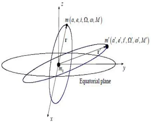
Having found the orbital elements at each moment in time we will use, we shall continue to describe the Moon’s third body perturbation affecting the upper stage on orbit. The system to be used to calculate the third body perturbation, in our case, the Moon, will be comprised of three bodies: one main body, the Earth, with mass 0, the second body, the upper stage with mass , and the third body, the Moon, with mass ′. The bodies are in this case assumed to be point

masses. The third body is in a three-dimensional Keplerian orbit around the main body having semimajor axis ′,

eccentricity ′, inclination ′, argument of pericentre ′, right ascension of the ascending node Ω′, and mean motion ′,

given by the general expression ′2 ′3= [ 0+ ′], where =6.67384∙10−11 3 −1 −2. The upper stage is in a three dimensional Keplerian orbit with semi major ,

eccentricity , inclination , argument of pericentre , right ascension of the ascending node Ω, and mean motion , given by the general expression 2 3= 0. The general form of the disturbing potential is shown in (43). The disturbing function of the third body influence is shown in (44), in the form of the Legendre polynomials expansion truncated up to the second order.

wherecos = ∙ ′ ′ and can be expressed as cos = cos + sin . and are two intermediate variables and are described in (46) and (47), with being the angle between and ′, =Ω−Ω′ being the difference of the perturbing

body’s and upper stage’s arguments of the longitudes and ′= ′+ ′, ′ being the perturbing body’s argument of latitude

and and ′ being the true anomalies of the upper stage and the perturbing body. The final form of the Moon’s third body perturbation affecting the upper-stage’s orbit and which will be used in the numerical simulations is denoted by (45).

The Sun’s orbit, Sun’s orbital elements and its third body perturbation upon the upper stage shall be described in a similar manner.

VI. PASSIVE ELECTROMAGNETIC TETHER DRAG

In (48), represents the resistivity and is the density of the conducting material of which the tether is made of. The tether’s resistance transforms this resulting power into heat, power which is then radiated away into space. This way, kinetic energy is extracted from the spacecraft. As specified in [8], a typical mass percentage of the tether, relative to the host spacecraft would be 1%. For an aluminium tether with mass =15 , resistivity =27.4 Ω ⁄ and density =2700 3⁄ , orbiting above the equator at a velocity of =7000 ⁄ relative to the Earth’s transverse magnetic field =20 , the power which will be dissipated will be =2650 . We can use this value, coupled with (49), to find out the time needed to lower a spacecraft’s circular orbit from radius 2 to radius 1 (with 2> 1. In (49), represents the spacecraft circular orbit’s semi-major axis, ⊕ is the Earth’s gravitational parameter, is the mass of the spacecraft and is the power dissipated by the drag force, given in (48). If we choose =1000 , 2=7378 , 1=6628 (a spacecraft descending from an orbit of initial altitude relative to Earth’s surface of 1000 km, to a final

altitude of 250 km), we get Δ =14.08 days.

The Earth’s magnetic field can be approximated by a magnetic dipole with the magnetic axis of the dipole tilted off from the spin axis of the Earth by =11.5 degrees. Using this magnetic dipole model, the magnetic field can be divided at any point in two components: a tangential, or horizontal component, , and a radial, or vertical component, .

In (50) and (51) represents the magnitude of Earth’s magnetic field on the magnetic equator at the surface of the Earth and is equal to 31 or 0.31 , =6378 is Earth’s radius, is the radial distance of a point from the centre of the Earth and is the magnetic latitude starting from the Earth’s magnetic equator. The 436 km offset of the magnetic dipole center from Earth’s center will not be taken into account. The calculations will be made with respect to the magnetic dipole frame of reference so the orbit inclination will have the formula = ± , where λ is the inclination

between the orbit and the plane of the magnetic dipole frame of reference, is the angle between the orbit and Earth’s frame of reference’s plane and is the angle between Earth’s plane of reference axes and the magnetic dipole frame of reference axes. The values of the inclination go from = + to =− once a day, as the upper stage orbits the Earth.

The motion of the tether across the geomagnetic field induces an electric field in the reference frame moving with the tether:

E = -υ × B (52)

Consequently, in the reference frame of the tether there will be a voltage along the tether: V = E .L (53)

By coupling (51), (52) and (54) into (54) and keeping in mind that = , now that we are doing the calculations in the magnetic dipole’s frame of reference, we get the following formula for the voltage along the tether:

The hallow cathode plasma contactor, field emission device, or bare wire anode, mounted at the end of the tether provides contact with the ambient plasma to the tether and allows current to flow through it. The tether material has a total resistance . This total resistance includes tether resistance, control circuit resistance, plasma contact resistance and parasitic resistances. The induced current flow through the tether will have the following formula:

ˆ

V

I

L

R

=

(56)

The movement of the tether, through which an electrical current flows towards the upper stage launch vehicle body, through Earth’s magnetic field, will generate an electrodynamic force (Lorentz force) on each element of the tether. When this force is integrated along the length of the tether, the net electrodynamic force will be:

Because of the tether’s movement on orbit, an electrodynamic drag force also appears, as component of the electrodynamic force , being parallel but opposite in direction to the velocity vector. This electrodynamic drag force

has the following formula:

VII. ATMOSPHERIC DRAG

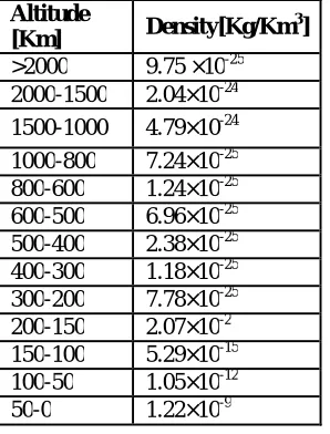
Table1. Atmospheric density variation with altitude

Table 2. Initial orbital elements of the Moon and the Sun

VIII. NUMERICAL SIMULATION AND RESULTS

For the numerical simulation in Matlab R2013a, the starting assumptions were considered. A tolerance of 10−8 was

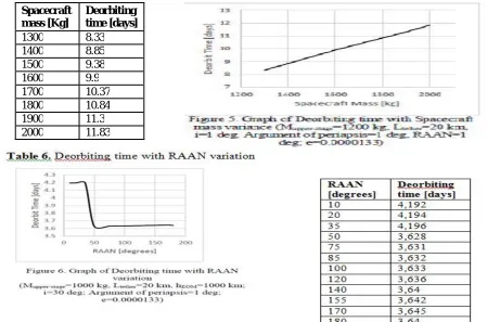
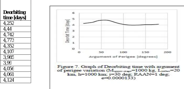
used within the ode45 solver, the integration time was considered to be 1 year, with a time step of 5 seconds. An aluminium electromagnetic tether of 20 km length was initially considered while the mass of the whole system (upper stage with electromagnetic tether and tether release mechanism) was taken to be 1000 kg. In Tables 3 – 8 and Figures 3 – 8 the deorbit times are shown with respect to the variation of the mass of the upper-stage, the initial orbital elements at end of mission and the length of the tether. While initial altitude, upper-stage mass, orbital inclination and tether length significantly affect the deorbit times, the RAAN and argument of periapsis variation have no observable influence over the deorbit efficiency.

Altitude

[Km] Density[Kg/Km

3

]

>2000 9.75 ×10-25 2000-1500 2.04×10-24 1500-1000 4.79×10-24 1000-800 7.24×10-25 800-600 1.24×10-25 600-500 6.96×10-25 500-400 2.38×10-25 400-300 1.18×10-25 300-200 7.78×10-25 200-150 2.07×10-2 150-100 5.29×10-15 100-50 1.05×10-12 50-0 1.22×10-9

Parameter Name Value for the Moon

Value for the sun

Unit of measure Eccentricity 0.0549 0.0167 n/a Semi-major Axis 3.86E+05 149.6+6 Km Inclination 28.58 23.4 Degrees Argument of

periapsis 318.15 102.947 Degrees Argument of

Table 4. Deorbiting time with Orbital inclination variation

Table 5. Deorbiting time with Spacecraft mass variation

Orbital inclination [degrees]

Deorbiting time [days]

10 15 6,89 20 7,05 25 7,18 25 7,46 30 7,81 35 8,25 40 9,08 45 9,88 50 11,03 55 12,04 60 13,18 65 14,41 70 16,53

Spacecraft mass [Kg]

Deorbiting time [days]

Table 7. Deorbiting time with argument of perigee variation

Table8. Deorbiting time with tether length variation

IX. CONCLUSIONS

The results presented in the last chapter conclude the efficiency of the electromagnetic tether deorbit device for an upper-stage in LEO at EOM, having reduced theoretically the deorbit time significantly, while taking in account the perturbations upon the upper-stage’s deorbit trajectory for a more realistic deorbit scenario. The simulations done with variance of the orbital elements, upper-stage mass and electromagnetic tether length have shown significant influence in deorbit time. Further improvements of the numerical simulations code and electromagnetic tether device analysis include taking into account of the influence of different tether materials and architecture higher numerical simulation accuracies and simulations which show how the orbital elements vary during the upper-stage deorbit.

REFERENCES

1. Hildreth AS, Arnold A, Threats to U.S. National Security Interests in Space: Orbital Debris Mitigation and Removal 2014.

2. Liou JC, USA Space Debris Environment, Operations, and Measurement Updates, 52nd Session of the Scientific and Technical Subcommittee Committee on the Peaceful Uses of Outer Space, United Nations, 2- 2015.

3. Matney M, The Challenge of Orbital Debris. 4. Orbital Debris Quarterly News, 2015; 19:7.

Orbital argument Perigee [degrees] Deorbiting time [days]

10 4,252 30 4,44 45 4,742 65 4,773 85 4,352 100 4,107 115 3,985 135 3,99 150 4,056 165 4,061 180 4,124

Tether length [Km] Deorbiting time [days]

5. Orbital Debris Quarterly News, 2007;11: 3.

6. Cosmo ML and Lorenzini (eds) EC, Tethers in space handbook, Third edition, Smithsonian Astrophysical Observatory, Cambridge, Massachusetts, USA, 1997.