A method for estimating the extent of denitrification of Arctic polar vortex air from tracer-tracer scatter plots

A method for estimating the extent of denitrification of arctic

polar vortex air from tracer-tracer scatter plots

J. G. Esler

Department of Mathematics, University College, London, England, UK

D. W. Waugh

Department of Earth and Planetary Sciences, Johns Hopkins University, Baltimore, Maryland, USA

Received 12 July 2001; revised 10 October 2001; accepted 11 October 2001; published 4 July 2002.

[1] A method for estimating the extent of denitrification of Arctic polar vortex air is

proposed. Previous estimates of denitrification using tracer-tracer scatter plots have not allowed for mixing-induced changes in tracer-tracer relationships in a sufficiently general way. This difficulty is overcome by constructing an artificial ‘‘reference tracer’’ from a linear combination of other long-lived tracers. The reference tracer is designed so that, as far as possible, it has a linear canonical relationship with NOy in midlatitudes. A linear relationship is unaffected by mixing, so denitrification is apparent as deviations of vortex measurements from the linear midlatitude relationship. The method is first demonstrated using data from a chemical transport model in which no denitrification processes are present. It is then applied to balloon, aircraft and shuttle-borne measurements made before and during the breakdown of the Arctic vortex in 1992 – 1993 and 1996– 1997. In each case the method indicates that little or no denitrification had occurred in any of the vortex air encountered. When the method is applied to the southern hemisphere vortex in 1994, by contrast, denitrified air is clearly seen to be present around 19– 23 km in the

vortex. INDEXTERMS:0340 Atmospheric Composition and Structure: Middle atmosphere—composition and chemistry; 0341 Atmospheric Composition and Structure: Middle atmosphere—constituent transport and chemistry (3334);KEYWORDS:denitrification, stratosphere, scatter plots, Arctic, vortex

1. Introduction

[2] The extent of denitrification and ozone loss in Arctic polar vortex air exhibits large interannual variability, which is due to the strong temperature dependence of the processes involved. Denitrification can be defined as irreversible removal of the nitrogen family NOy, where

NOy¼HNO3þHNO4þNOþNO2þClONO2þ2N2O5:

ð1Þ

Denitrification occurs through the sedimentation of HNO3 -bearing polar stratospheric cloud (PSC) particles, and these form at low temperatures during winter in the Arctic region. Significant denitrification leads to an increase in the lifetime of ozone-depleting chlorine species (ClOx), and therefore

leads to an increase in the duration and extent of springtime Arctic ozone loss. It has been suggested that slight cooling in the Arctic due to climate change could lead to enhanced denitrification in the future, and this could lead to larger seasonal ozone depletion, despite the projected decline in inorganic chlorine [Waibel et al., 1999; Tabazadeh et al., 2000].

[3] Small uncertainties in analyzed temperatures make quantitative modelling of denitrification subject to poten-tially large errors. This makes it particularly important that

denitrification can be inferred from direct observations. However, transport processes in the stratosphere mean that it is not possible to directly compare measurements at a given location with those made earlier in the winter. Instead, some authors have exploited the fact that long-lived tracers in the stratosphere tend to exhibit compact, robust relation-ships [Fahey et al., 1990;Plumb and Ko, 1992].

[4] Fahey et al. [1990] andRinsland et al. [1999] have both used the standard midlatitude NOy:N2O relationships to predict NOyconcentrations in the absence of denitrification

processes and interpreted deviations from this relationship in vortex measurements as being due to denitrification. Other authors have used a similar approach to estimate chemical ozone loss [Proffitt et al., 1990; Mu¨ller et al., 1996, 1997]. However, it has also been recognized that tracer relationships can also be altered by mixing processes, and deviations from standard relationships between long-lived species have been attributed to mixing byWaugh et al.[1997a] andMichelsen et al.[1998a, 1999]. Following this reasoningMichelsen et al. [1998b] and Kondo et al. [1999] attribute measured deviations from the standard midlatitude NOy:N2O relation-ship as being due to mixing rather than denitrification.

[5] An attempt to distinguish between mixing and deni-trification effects on the NOy:N2O relationship was recently made by Rex et al. [1999]. They analyzed data from the 1996 – 1997 and 1992 – 1993 northern winters, much of which will be further treated in this paper. Treating CH4 and N2O as long-lived species, they estimated the amount of Copyright 2002 by the American Geophysical Union.

0148-0227/02/2001JD001071

mixing undergone by vortex air by using the deviation from the standard midlatitude CH4:N2O canonical relationship. From this information the change to the standard NOy:N2O relationship due to mixing alone was estimated, and any remaining discrepancy with the observed NOy:N2O ratio was attributed to denitrification. They recognized, however, that their estimation of the mixing effect was dependent on their assumption that the ex-vortex air had undergone a single mixing event near the level at which it was observed (scenario A below). Comparing late winter measurements within the vortex with later measurements in filaments during the 1992 – 1993 winter/spring, Plumb et al. [2000, hereinafter referred to as PWC], argued that most mixing had in fact taken place before the vortex breakup. They suggested that midlatitude air may have been mixed into the vortex intermittently at several levels during the winter (scenario B below). If theRex et al.[1999] method is used in this case, PWC argued that using different long-lived tracers to esti-mate the mixing effect might yield different results.

[6] In section 2 the two mixing scenarios mentioned above are discussed, concentrating on their effect on tracer-tracer relationships. We then describe a method for determining denitrification (and irreversible loss in general) from direct measurements, in the presence of mixing of any kind. The information from the measurements of several long-lived tracers is exploited to account for the change in NOy

concentration due to mixing alone, as far as this is possible. The method is then applied to both chemical transport model data in section 3 and aircraft, balloon, and shuttle-borne measurements in sections 4 and 5. Our conclusions, as well as brief discussion of the possible application of the method to chemical ozone loss, are given in section 6.

2. Mixing Scenarios and the Reference Tracer Method

[7] In regions of the stratosphere where the following two conditions are satisfied, the isopleths of long-lived tracers become coincident and a tracer-tracer scatter plot of any two tracers shows a compact relationship (i.e., points on a scatter plot lie upon a straight or curved line.) The two conditions are the following [Plumb and Ko, 1992;Plumb, 1996]:

1. The timescale for transport along rapid exchange surfaces (in this case isentropic surfaces) is much faster than the timescale for transport across those surfaces.

2. The timescale for transport along isentropic surfaces is much faster than the local chemical timescale.

[8] These conditions are satisfied both in the winter midlatitude stratosphere and arguably in the interior of the polar vortex (although not in the vortex edge region) for long-lived species, e.g., N2O, NOy, CH4, and CFCs. If two species have everywhere spatially similar sources and sinks the relationship between them will be linear, that is, a scatter plot of measurements of both species will lie on a straight line. Differences in the spatial structure of sources and sinks lead to nonlinearity in tracer relationships, that is, curvature in the correlations between them.

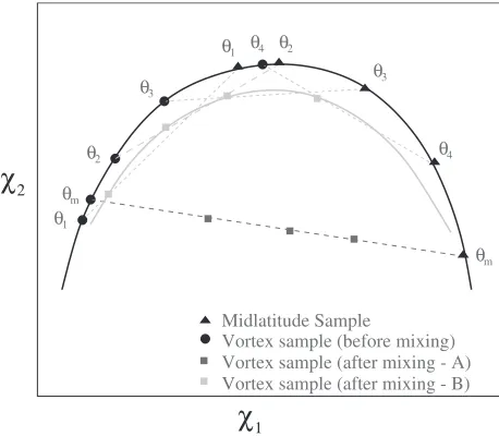
[9] The black curve in Figure 1 shows a hypothetical, nonlinear, canonical tracer-tracer relationship between two long-lived speciesc1andc2. At the beginning of the winter this relationship is expected to hold both inside and outside the polar vortex.

[10] During the winter, air within the vortex descends. If there is no mixing for a prolonged period the canonical c2:c1relationship still holds everywhere. If there is then a single mixing event, which we shall call scenario A, at level qmbetween the vortex and midlatitudes, the mixed air will

lie on an anomalous mixing line, illustrated by the dark grey dashed line, in tracer space.

[11] Mixing scenario B is that of continuous mixing. The grey curve and dotted lines illustrate how the vortex relation-ship evolves if there are mixing events at many levelsq1–q4 in midwinter. The mixing causes the vortex relationship to become distinct from that of the midlatitudes, which is less easily altered by mixing with the vortex (due to the greater area of the midlatitudes). Further mixing may then cause the vortex relationship to become yet more distinct.

[12] In principle, the information from several conserved tracers can be combined to reveal information about the mixing history of observed air parcels. A parcel descending in the vortex may have been mixed with extratropical air at several levels, changing its NOyconcentration even in the

absence of chemistry. It is therefore helpful to define [NOyy]

to be the expected concentration of NOyin an air parcel in

the absence of chemistry. Since long-lived tracers such as N2O, CH4, CFC-11, CFC-12, and CFC-113 have also undergone mixing, we might hope to predict [NOyy] using

information derived from the change in their canonical relationships. [NOyy] is essentially equivalent to [NO**]y

defined by Rex et al. [1999] but will be estimated by the method to be described.

[13] If a conserved tracer happened to have a linear canonical relationship with NOy at the beginning of the

winter, the situation is less complicated. Instead of causing

Figure 1. The effect on the canonical tracer-tracer relation-ship between long-lived species c1 and c2 of different mixing scenarios. In scenario A, no mixing takes place between vortex and midlatitude air until late in the winter when a single mixing event takes place on the isentropic level qm. Samples of mixed air then lie along the dark grey dashed

departures from the canonical relationship, mixing can only move parcels along it in tracer space. [NOyy] can therefore be

read directly from the canonical relationship, and denitrifi-cation is given by [NOyy][NOy].

[14] Unfortunately, no such tracer exists. However, we shall show in what follows that an artificial tracer (X) may be constructed by adding together a linear combination of long-lived tracers, in order to form a tracer which has, as near as possible, a linear relationship with NOy. We shall

refer to this tracer as the ‘‘reference tracer.’’ Note that as the reference tracer is constructed from long-lived tracers it will also be long-lived. Because it is a linear combination of other tracers, it undergoes linear mixing like any of its constituent tracers. Using this tracer, we can estimate [NOyy]

and denitrification.

[15] The method we used for constructing the reference tracer (X) is described in Appendix A. Our starting point was to obtain midlatitude canonical correlations between all the species to be used in each case and N2O. These relationships were then used as a guide to constructing the reference tracer. This was done by forming a set of simultaneous equations in the tracer coefficients, that were equivalent to forcing the midlatitude NOy:X relationship to intersect the straight line

[NOy] = [X] at several points. The positions of these points

were chosen by trial and error for best results.

[16] The result in each case is a double-valued canonical relationship. This can be expressed as functions of [X], i.e., [NOy]+ ([X]), and [NOy] ([X]). The two branches

correspond to the [N2O] ranges [N2O] > [N2O]M and

[N2O] < [N2O]M respectively, where [N2O]M (approx

40 – 65 ppbv) is the N2O concentration associated with the maximum NOy concentration in the mid-stratosphere.

Both of these branches lie on or close to the straight line [NOy]=[X] for the range of [N2O] values over which mixing is likely to take place. This canonical relationship can be used to estimate [NOyy] for vortex measurements

that may have undergone denitrification, using

½NOy_y ¼ ½NOyð½X Þ ½X ð2Þ

for the measured (X). The plus or minus branch is chosen depending on whether or not [N2O] > [N2O]M. The

appropriate estimate for denitrification is then simply [NOyy][NOy].

[17] It is important to emphasize that the initial canonical relationships are used merely as an aid to obtaining a linear NOy:X relationship; i.e. they are not necessary for its

construction. If the initial canonical relationships used do not accurately fit the data, then the data points need not lie along the calculated NOy:X canonical relationship. The

need for initial canonical relationships may be avoided by instead using a least squares fit of the data. In this method the coefficientsatoeof the reference tracer are obtained by finding those values ofatoethat minimize a function with the form

fða;b;c;d;eÞ ¼Xða½N2O þb½CH4 þc½CFC11

þd½CFC12 þe½NO

yÞ2: ð3Þ

Here the sum is taken over all the available midlatitude or early winter data. Note that for this method to work the data must cover the entire [N2O] range over which mixing may

occur. Regions of sparse data may need to be positively ‘‘weighted’’ when the sum is taken, and data points derived from canonical correlations might be used where data is absent. Provided this is not necessary, however, this alter-native method bypasses the need to use canonical relation-ships in deriving the tracer coefficients.

3. Application to Chemical Transport Model Results

[18] In this section the reference tracer method will be applied to results from a chemical transport model experi-ment [Waugh et al., 1997b; PWC]. No denitrification processes are included in the model chemistry, so NOy

behaves as a long-lived tracer throughout the model experiment (i.e., [NOyy] = [NOY]). Figure 2a shows a

typical midlatitude NOy:N2O scatter plot. The red, orange, and yellow points are samples from the Northern Hemi-sphere midlatitudes, colored according to their N2O concen-tration, taken from the 1 March results. The samples form a fairly compact canonical correlation for the model midlati-tudes, and the canonical curves shown on this and subse-quent plots are fits to this data. Also on this plot are blue and cyan points showing samples from the model arctic vortex on 1 April (blue- below 35 mbar level, cyan- above 35 mbar level). In the range 5 < [N2O] < 150 ppbv the vortex samples lie significantly below the midlatitude correlation. Prior to the vortex forming, the midlatitude and high-latitude NOy:N2O relationships are similar (PWC). The change cannot be due to denitrification as none has been included in the model chemistry, so it must be due to mixing. In fact, as shown in PWC, high [N2O] midlatitude air is mixed into the vortex throughout the winter in the model (scenario B above), causing the NOy:N2O relationship to change inside the vortex. Although there is also mixing of low [N2O] air out of the vortex, the much greater volume of the midlatitude surf zone means that the midlatitude NOy:N2O relationship barely changes.

[19] A contrasting picture can be obtained by using a reference tracer that has been constructed to be, as near as possible, linear in its canonical correlation with NOy. We

have constructed three different reference tracers from different combinations of long-lived tracers as shown in Table 1. Looking first at the NOy:X relationship in Figure

2b, the lack of significant deviations of the modelled data from a straight line demonstrates that no real denitrification is taking place. The tracer X is defined by the combination

X

½ ¼0:0335 CH½ 4ppbþ0:0040 CFC½ 11ppt

0:0393 CFC½ 12

ppt0:125 N½ 2Oppbþ8:759: ð4Þ

The NOy:X canonical correlation is close to being linear in

the midlatitudes for the range 300 ppbv > [N2O] > 6 ppbv, i.e., the red and orange points. Mixing between any two points in tracer space, with 300 ppbv > [N2O] > 6 ppbv, cannot cause significant departure from the canonical relationship. In Figure 2b the blue points from the vortex (below the 35 mbar level) lie along the NOy:X canonical

relationship. These are the same points that from a naive reading of Figure 2a might have been thought to represent denitrified air. The reference tracer method therefore proves directly from the model data that [NOy] [X] and no

[20] The light blue points in Figure 2a (not plotted on Figure 2b) are vortex samples measured on model levels above the 35 mbar surface. Most of these happen to have undergone mixing with air that originally had [N2O] < 6 ppbv, so it is not appropriate to use the NOy:X plot to distinguish

between denitrification and mixing for these points. In fact, they lie below the canonical curve in Figure 2b. Those orange points that do fall below the canonical curve in Figure 2b have also mixed with air that has [N2O] < 6 ppbv. (The points that lie above the curve have mixed with tropical air, which has separate distinct canonical correlations and therefore does not lie on [NOy] [X]). Clearly, the range in N2O space that the NOy:X midlatitude canonical relationship

remains linear is important, as the method cannot be applied when mixing with air that contains N2O concentrations outside the linear range has occurred. Perhaps surprisingly, we shall show in the next section that it is easier to construct a reference tracer that is linear with NOyto higher levels (1 – 3

ppbv [N2O]) with observed canonical correlations than it is with the CTM canonical correlations. This may be because of model lid effects in the CTM. The problem of limited applicability in altitude of the reference tracer method is therefore less problematic in the observational data sections that follow. The altitudes at which it is most important to be able to distinguish between mixing and denitrification effects are 18 – 22 km (below 50 mbar) [Kondo et al., 1999]. An important question for the method is whether or not a significant mass of air that has low N2O concentration, outside the linear range for the reference tracer, descends to this level over the course of the winter. Comparing vertical descent rates and vertical profiles of N2O [Schmidt et al., 1991;Bauer et al., 1994;Abrams et al., 1996b], the possi-bility that some mesospheric air with very low N2O reaches the 18 – 22 km level by the end of the winter cannot be completely ruled out. However, the absence of any hint of mixing lines with very low N2O air in any of the tracer data that we present here makes this seem unlikely for both the CTM data and the relatively warm winters, with correspond-ingly weak descent, of 1992 – 1993 and 1996 – 1997.

[21] Applying the method with a second combination of tracers,

Y

½ ¼0:0303 CH½ 4ppbþ0:030 CFC½ 11ppt

0:272 CFC½ 113

ppt0:119 N½ 2Oppbþ9:06 ð5Þ

yields very similar results (Figure 2c). We shall show in the following sections that it is useful to have more than one

possible combination when using observational data, because of variations in the range of applicability in altitude and error sensitivities when using different species. We have also exploited the fact that the CFC-11 coefficient in the definition of X (equation (4)) is effectively fairly small, by defining Z to be equal to X without a CFC-11 component; that is,

Z

½ ¼0:0335 CH½ 4ppb0:0393 CFC-12½ ppt

0:125 N½ 2Oppbþ8:759: ð6Þ

Again, this yields similar results (not shown), with the obvious advantage of requiring only three (rather than four) simultaneously measured species.

[22] Figure 3 show scatter plots of the species that make up X, Y, and Z with N2O, CFC-11:N2O (Figure 3a), CH4:N2O (Figure 3b), CFC-113:N2O (Figure 3c), and CFC-12:N2O (Figure 3d). In each panel it is clear that the blue vortex points lie on the concave ‘‘mixing’’ side of the midlatitude canonical correlation traced out by the orange and red points. That is, the blue points lie below the canonical correlation in the case of CH4:N2O, and above it for CFC-11:N2O, CFC-12:N2O, and CFC-113:N2O. It is clear, particularly from Figures 3a and 3c, that the vortex points do not lie along a single straight mixing line, illustrating that midlatitude air must have mixed into the vortex during several mixing events and/or by continuous weak mixing as suggested by PWC for this CTM experi-ment.

[23] The grey curves in Figures 2a and 3a – 3d represent reasonable bounds on the scatter of the midlatitude canon-ical correlation of the four species with N2O. If the devia-tions from each of these four midlatitude reladevia-tionships were completely independent from each other at every CTM grid point, the scatter in the NOy:X plot would be given by the

grey curves in Figure 2b; that is, it would be around 4 ppbv of NOy. However, the NOy:X scatter is actually much less

than the NOy:N2O scatter in the CTM. We believe the reason for this is most of the CTM scatter is due to weak vortex-midlatitude mixing, and the reference tracer method accounts for much of this just as it accounts for the stronger mixing into the vortex. However, this does mean that scatter caused by genuinely independent errors such as instrument inaccuracy will be greater for NOy:X than NOy:N2O. It is therefore difficult to place a priori bounds on the scatter in the NOy:X relationship, as ‘‘mixing scatter’’ will exist in the

real atmosphere as well as in the CTM. The actual scatter must necessarily be obtained by simply plotting out the reference NOy:X relationship.

[24] The above method works by efficiently combining the extra information on mixing history of an air parcel contained in the ratios of the long-lived species, e.g., CFC-11:N2O, CFC-113:N2O, and CH4:N2O. Each of these ratios

Figure 2. (opposite) Tracer-tracer scatterplots from the chemical transport model experiment ofWaugh et al.[1997b]: (a) NOy:N2O, (b) NOy:X, and (c) NOy:Y. The yellow-orange-red points are typical midlatitude samples from 1 March, (yellow,

[N2O] < 6 ppbv; orange, 4 ppbv < [N2O] < 40 ppbv; red, [N2O] > 40 ppbv). The cyan-blue points are vortex measurements from 1 April (cyan, p < 35 mbar; blue, p > 35 mbar). The black arrows in Figure 2a indicate ‘‘apparent denitrification.’’ Standard midlatitude canonical correlations are plotted as black curves and grey curves mark bounds on the scatter. The same points are plotted on each panel. See color version of this figure at back of this issue.

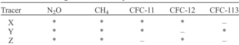
Table 1. Showing Constituents Species for Each Reference Tracer

Tracer N2O CH4 CFC-11 CFC-12 CFC-113

X * * * * –

Y * * * – *

is most sensitive to mixing between air masses with particular N2O concentrations. For example, as can be seen from Figure 3, CFC-11:N2O changes most rapidly when air with [N2O] > 130 ppbv mixes with air that has [N2O] < 130

ppbv, for CFC-113, the CFC-113:N2O ratio is most sensi-tive to mixing around [N2O] = 90 ppbv, CFC-12, 50 ppbv and CH4, 40 ppbv. The NOy:N2O ratio is most sensitive to mixing in the range 40 – 50 ppbv, so it is perhaps not

Figure 3. Tracer-tracer scatter plots from the chemical transport model experiment of Waugh et al.

surprising that CH4 and CFC-12 are key components in most of the tracers cited above, with CFC-11 possibly the least important component in each case, which is why it can be dropped when defining Z. The advantages and disadvan-tages of using of CFC-12 as opposed to CFC-113 are discussed in the following section. Attempts to define a reference tracer without using CH4as one of the constituent species did not result in a reference tracer that was linear with NOyacross much of the required range in N2O space. [25] Comparing two locations with the same N2O mix-ing ratio (64 ppbv), one from the vortex and one from the midlatitudes, the vortex location has the lower NOy

con-centration (16.2 ppbv compared to 19.1 ppbv) due to mixing. However, the same mixing has also caused the vortex [CH4] to be lower (568 to 641 ppbv), making its [Y] value lower by 2.22. Mixing has also increased the vortex [CFC-113] relative to midlatitudes (8.24 pptv to 5.39 pptv) causing the vortex [Y] to be a further 0.78 lower. The higher [CFC-11] in the vortex has the reverse effect, adding 0.15 to [Y]. The contributions from each species ensure that [Y] [NOy] both inside and outside

the vortex, with the change in CH4 the most important component in this example. However CH4, CFC-11, and CFC-113 make a more equal contribution to the change in [Y] when [N2O] = 120 ppbv.

4. Application to POLARIS Data

[26] During the spring and summer of 1997 a series of ER-2 aircraft flights and several MkIV balloon flights were made into the Northern Hemisphere extratropical lower stratosphere during the Photochemistry of Ozone Loss in the Arctic Region in Summer (POLARIS) mission [ New-man et al., 1999]. Vortex remnants with low N2O concen-trations (<150 ppbv) were encountered on several occasions during the mission at the ER-2 flight altitude, typically around 22 km, most notably on the flights of 26 April, 26 June, 29 June, and 30 June. Numerous species were measured by on-board instrumentation including NOy,

N2O, O3, CH4, CFC-11, CFC-12, and CFC-113.

[27] The MkIV balloon flights (MkIV Fourier Transform Infrared (FTIR) Interferometer [Toon et al., 1999]) we will examine occurred on 8 May, 8 July, and 9 July 1997 from Fairbanks, Alaska (64.5N, 147W). The balloon measure-ments are included as they extend up to a much greater altitude (38 km) compared with the aircraft data. We have concentrated on using measurements of N2O, CFC-12, CH4, and NOy. We use NOy calculated from the directly

observed HNO3, NO, NO2, N2O5, ClONO2, and HNO4(see equation (1)).

[28] We make the same basic assumption about the treatment of the ER-2 and MkIV data sets as Rex et al.

[1999], namely that two data sets can be compared directly without correction for systematic differences. Good agree-ment has been demonstrated between ER-2 and MkIV data for midlatitude NOy and N2O, [Sen et al., 1998], and for N2O, NOy, CH4and CFC-12 [Toon et al., 1999]. Measure-ment accuracies for each species [Toon et al., 1999] are NOy

(10%, 15%), N2O (2%, 5%), CH4(3%, 5%), CFC-11 (2%, 10%), CFC-12 (2%, 10%), and CFC-113 (3%, 20%), where the first number in brackets in each case is the ER-2 error and the second the MkIV error. We do not use MkIV

CFC-113 measurements in what follows because of the large bias between these and the ER-2 measurements [Toon et al., 1999].

[29] Comparison of the ER-2 and the ATMOS data, discussed in section 4 below, is also given byChang et al.

[1996], for CH4, NOy, and N2O. Note that ATMOS data are obtained using a similar solar occultation method to MkIV data. The reader is referred toRex et al.[1999] for further discussion of these issues. We choose the Airborne Chro-matograph for Atmospheric Trace Species (ACATS) instru-ment [Elkins et al., 1996] for our calculations involving ER-2 N2O and CH4, as this instrument is also used to simulta-neously measure the CFCs.

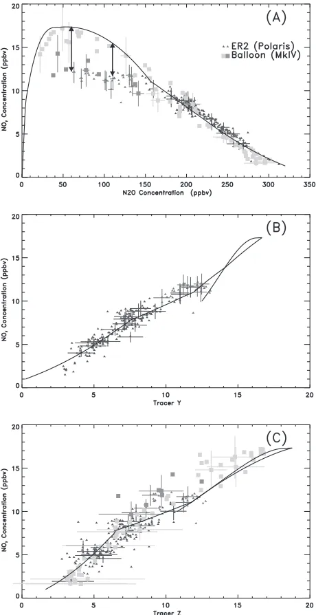
[30] Applying the reference tracer method described above to these data, we can make inferences about the degree of denitrification present in the air encountered during the above aircraft and balloon flights. Figure 4a shows the NOy:N2O scatter plot obtained from these data. The black curve denotes the midlatitude canonical correla-tion curve for these two species. The shape is identical to that given byMichelsen et al.[1998b] for ATLAS data but with some slight rescaling of axes to obtain a better fit to this different data. Balloon measurements are plotted as green and orange squares and aircraft measurements as blue and cyan triangles. The coloring has been chosen so that green and cyan points correspond to ‘‘apparently denitri-fied’’ air, i.e., air with N2O and NOyconcentrations located

significantly below the level of the midlatitude NOy:N2O canonical correlation. Orange and blue points denote sam-ples of ‘‘typical’’ midlatitude air that lie on or near the canonical correlation curve.

[31] Figure 4b shows the aircraft data only, plotted as an NOy:Y scatter plot, where Y in this case is given by

Y

½ ¼0:0179 CH½ 4ppb0:040 CFC-11½ ppt

0:187 CFC-113½ ppt0:0530 N½ 2Oppbþ4:9: ð7Þ

Note that it is necessary to use slightly different coefficients for Y compared with the CTM results above, because the CTM and observed canonical correlations differ fairly significantly. The black NOy:Y canonical

aircraft measurements of filaments (during the SPADE campaign [Wofsy et al., 1994]).

[32] Figure 4c shows similar results for NO_y:Z, where

Z

½ ¼0:0371 CH½ 4ppb0:0466 CFC½ 12ppt0:1 N½ 2Oppb5: ð8Þ

The NOy:Z plot reveals a greater scatter than NOy:Y (see

discussion below), but it has the advantage that Z can also be calculated for the MkIV data. (Another advantage is that this correlation remains near linear up to [N2O] 1 – 2 ppbv, meaning that the NOy:Z correlation is relatively unaffected

by mixing with air originating at higher levels compared with Y.) All the points on Figure 4c remain close to the canonical curve. Similar conclusions can therefore be drawn from Figure 4c as from Figure 4b, this time for both the ER-2 and the balloon data. The balloons have encountered layers of old vortex air at and above the height of the ER-2 flights, and the large deviations from the midlatitude NOy:N2O canonical correlation present these can again be accounted for by mixing alone. The greater scatter in this plot, however, means that the Z analysis can bound the level of possible denitrification to within only 1 – 2 ppbv or so.

[33] Error bars on Figure 4 show the (1s) accuracy of the instruments measuring each species. For Y and Z the 1s error bars are calculated assuming that the errors associated with each component are independent. The error bars for the balloon measurements of Y and Z in particular are large, especially for low values, and this sensitivity is due to the large degree of cancellation between the [CH4] and [N2O] components of Y and Z at low values.

[34] Figure 3 shows scatterplots of ER-2 and MkIV measurements of each of the species used to calculate Y and Z. In the case of CH4:N2O the canonical relationship is a rescaled version of the polynomial fit given byMichelsen et al.[1998b]. In the case of the CFCs the canonical relation-ships plotted are linear fits to the midlatitude data in the lower stratosphere, matched to quadratic fits in the mid-upper stratosphere where the CFC concentrations decay to negli-gible concentrations. The color coding of the points allows some insight into why the reference tracer method has indicated that mixing (rather than denitrification) has taken place. Green and cyan points that correspond to measure-ments of old vortex apparently denitrified air appear, in nearly every case, on the mixing side of each canonical correlation (i.e., below the black curve in Plate 4A, and above the black curves in Figures 4b – 4d). The orange and blue midlatitude samples lie on or near the curve. (The few points that are clear exceptions to this statement, mostly among the MkIV CFC-12 measurements, are responsible for the outlying points in Figure 4c.) The fact that the air represented by the cyan and green samples has undergone this mixing is reflected in the calculated values of Yand Z and is the reason that the cyan and green points remain near the canonical curves in Figures 4b and 4c.

[35] The vortex ER-2 measurements (cyan points) can be seen to lie on two separate lines in each of Figures 5a – 5d, as well as in Figure 4c (NOy:N2O). These correspond to separate flights, one in April, when the vortex was measured directly, and one in June when vortex remnants were measured. The June samples appear in each case to have undergone more mixing. When the same samples are plotted on the NOy:Y

plot the April and June measurements converge near the canonical curve, again illustrating the ability of the reference tracer method to account for different degrees of mixing.

[36] In summary the advantage of Z over Y turns out to be that it is easier to construct a tracer that is linear over a greater range in altitude (or equivalently N2O space) for Z compared with Y. However, the disadvantage with Z is that,

Figure 4. Tracer-tracer scatter plots of data collected during POLARIS (spring – summer 1997), including ER-2 and MkIV data: (a) NOy:N2O, (b) NOy:Y, and (c) NOy:Z.

comparing Figures 5b and 5d, the difference in the CFC-12:N2O ratio between vortex and midlatitude air is small compared with CFC-113:N2O. This means that NOy:Z is

more sensitive to scatter caused by (say) instrument error in measuring CFC-12 compared with NOy:Y, which explains

why there is greater scatter and larger error bars in Figure 4c compared with Figure 4b.

[37] These results provide a robust confirmation of the assertion byKondo et al.[1999] that the NOy:N2O measure-ments made in the ex-vortex air during this winter can be explained by mixing alone. However, as explained in

Kondo et al. [2000], satellite measurements showed that some denitrification did occur in the vortex, although much earlier than the POLARIS measurements (February 1997).

5. Application to ATLAS Data

[38] During the Atmospheric Laboratory for Applications and Science (ATLAS) shuttle missions, the Atmospheric

Trace Molecule Spectroscopy (ATMOS) instrument [Michelsen et al., 1998a, 1998b], was used to measure long-lived tracers in the northern hemisphere extratropical stratosphere during April 1993 (ATLAS-2) and November 1994 (ATLAS 3). Occultations during ATLAS 2 included measurements made inside the late winter vortex, identifi-able from vertical profiles with unusually low N2O in the midstratosphere, as well as measurements made in the midlatitudes. During ATLAS 3, similar midlatitude profiles were obtained as the Arctic vortex formed at the beginning of the 1994 – 1995 winter. We will use these latter data to help form standard midlatitude profiles for our reference tracer.Michelsen et al.[1998b] give the instrument accuracy for ATMOS to be 5% for N2O and CH4, and 6 – 16% for NOydepending on altitude, andAbrams et al.[1996a] quote

11% accuracy for CFC-11 and 9% accuracy for CFC-12. [39] Figure 6 shows the reference tracer method applied to the ATLAS data. The canonical correlations shown are the ATLAS midlatitude fits given by Michelsen et al. Figure 5. Tracer-tracer scatter plots from POLARIS: (a) CH4:N2O, (b) CFC-12:N2O, (c) CFC-11:N2O,

[1998b] and the CFC canonical relationships are linear/ quadratic fits as in Figure 4. The NOy:N2O scatter plot (Figure 6a) once again indicates apparent denitrification of the vortex measurements. If a reference tracer is used (Figure 6b), this time called X as CFC-11 and CFC-12 are both used

X

½ ¼0:0271 CH½ 4ppb0:0195 CFC½ 11ppt

0:0344 CFC½ 12

ppt0:0750 N½ 2Oppb0:05: ð9Þ

we see instead that both vortex (blue points) and midlatitude (green points, ATLAS 2; red points, ATLAS 3) observations fall close to the near linear midlatitude canonical relation-ship illustrated by the black curve. This is again strongly indicative that little or no denitrification has taken place during the winter 1992 – 1993 and that the apparent denitrification in Figure 6a is due to mixing. Error bars are omitted from this plate to avoid cluttering but are of a similar magnitude to the MkIV error bars shown on Figures 4a and 4c. Figures 6c – 6e show the measurements of the species making up X.

[40] The relative lack of simultaneous measurements of all four tracer X species in the ATLAS 2 data means, however, that some significant approximations were necessary in the construction of Figure 6b. Green and blue points marked by diamonds indicate that N2O and CH4 measurements were used to calculate X, but the remaining species were approxi-mated by [CFC-11]C and [CFC-12]C_{, respectively. Here}

[CFC-11]Cand [CFC-12]Chave been estimated from meas-ured [N2O] using the standard midlatitude canonical corre-lations (solid black curves in Figures 6c and 6e) for the midlatitude measurements (green points), and vortex canon-ical correlations (dotted black curves in Figures 6c and 6e) for the vortex measurements (blue points). By contrast, green and blue stars indicate that [N2O], [CFC-11], and [CFC-12] have been used along with [CH4]

C

. No such approximations were necessary for the ATLAS 3 data (red points).

[41] The use of the above approximations means that it is difficult to place a bound on the accuracy of the reference tracer method for this winter. It is possible that some denitrification (1 – 3 ppbv) may have occurred in some of the air encountered, but that this is not detectable owing to inaccuracy in the calculation of [X]. However it is notable from Figures 6c – 6e that the vortex measurements of CFC-11:N2O, CH4:N2O, and CFC-12:N2O nearly all lie on the mixing side of the midlatitude canonical correlation, just as with the CTM, POLARIS, and MkIV data (although there were very few ATLAS vortex measurements of CFC-11). This further supports the conclusion from the reference tracer method, also suggested by Michelsen et al.[1998b], that the vortex measurements of NOy:N2O during this winter can be explained by mixing alone.

[42] Figure 7a shows the NO_y:N₂O relationship during ATLAS 3 (November 1994) in the Southern Hemisphere. As the Antarctic vortex is colder than the Arctic, extensive denitrification takes place every year [Michelsen et al., 1998b]. Consistent with this, ATLAS 3 vortex measure-ments made entirely within the vortex (blue points), typi-cally have very low values of [N2O] (2 – 5 ppbv). Midlatitude samples (red points) follow a relationship similar to the northern hemisphere canonical relationship.

It is clear from the vertical N2O profiles that the green points that remain are derived from occultations that inter-sect the vortex edge at some altitude. Some of these points lie on the midlatitude relationship, while the rest show various degrees of apparent denitrification.

[43] Figure 7b shows the NOy:X relationship. Here X is

identical to equation (9) above. Note that the measurements in Figures 7a and 7b are further subdivided into measure-ments made below 19 km (stars), 19 – 23 km (squares), and above 23 km (triangles). It is notable that all the blue stars and squares lie significantly below the midlatitude NOy:X

relationship, marked out by all red points plus the green triangles. This confirms that the vortex occultations have measured air that is clearly denitrified up to 23 km, albeit by slightly less than is apparent from the NOy:N2O plot. Similarly, most vortex edge measurements below 19 km (green stars) also show denitrified air. However, between 19 and 23 km (green squares) these occultations have mostly measured air that appears denitrified on the NOy:N2O plot, but not on the NOy:X plot. This appears to be another

example of apparent denitrification due to mixing.

[44] Figures 7c – 7e contain further evidence that mixing into the vortex plays a role in the Southern Hemisphere. In each panel it is clear that the vortex measurements (blue points) lie to the mixing side of the midlatitude relationship defined by the red points. As with the NOymeasurements,

some green points have midlatitude characteristics and some vortex characteristics. The evidence for mixing is particu-larly clear in the CFC-11 plot, where vortex air with relatively low [N2O] values (50 – 100 ppbv) has significant levels of CFC-11 (10 – 20 pptv). This CFC-11 would be entirely absent if mixing of vortex and high N2O midlati-tude air had not occurred. This mixing is accounted for in Figure 5b and results in lower [X] and therefore lower calculated loss of NOy.

6. Discussion and Conclusions

[45] Given simultaneous measurements of NO_yand sev-eral long-lived species in (ex)-Arctic vortex air, we have described a method of obtaining a quantitative estimate of denitrification, even in the case where the vortex air has undergone a series of unknown mixing events with mid-latitude air. The method depends on creating a reference tracer, defined as a linear combination of long-lived species, that has a near-linear canonical relationship with NOy in

midlatitude air. Assuming that at the beginning of the winter the vortex air also has this near-linear relationship, mixing between descending vortex air and midlatitude air will not cause significant departure from this relationship. Denitrifi-cation can be quantified as the difference between [NOyy]

and [NOy] measured in the vortex, where [NOyy] is the

expected concentration of [NOy] at a fixed value of the

reference tracer.

[46] Applying this method to measurements made during the relatively warm winters of 1992 – 1993 and 1996 – 1997 our results have reinforced the arguments ofMichelsen et al.

denitrification did take place in other regions of the vortex during February 1997. One or two balloon flights also described byKondo et al. [1999] did pass briefly through air that they argued was denitrified. This method might have offered a way of quantifying this denitrification had more long-lived species been measured concurrently.

[47] Finally, it is worth discussing the possible applica-tion of this method, or some variaapplica-tion on it, to quantify chemical ozone loss in the Arctic. Some further problems must be overcome to achieve this. At the beginning of the winter the chemical timescale for ozone in midlatitudes is too short for compact relationships to form between it and longer-lived species (see Plumb and Ko’s condition (2) above). Compact relationships do form during the winter [Proffitt et al., 1990;Mu¨ller et al., 1996, 1997] but are likely to be different inside and outside of the polar vortex. If account is taken of these initially different relationships, and some midwinter vortex measurements are available to compare with later measurements during or after vortex breakup, then an analysis of the type described in this paper might be worthwhile.

Appendix A: Determining the Tracer Coefficients

[48] Our method for determining the tracer coefficients is as follows. First, the canonical correlations, which are fits to the compact relationships between long-lived tracers, are all expressed as a function of the concentration of the same species, in our case [N2O]. As NOyhas a maximum in the

midstratosphere, it is helpful at this point to define [N2O]M

as the concentration of N2O that corresponds to the max-imum concentration of NOy, defined as [NOy]M.

[49] Next, to obtain coefficients for a reference tracer made up of four species c1c4 (representing, e.g., N2O, CH4, CFC-11, CFC-113), we solve the five simultaneous equations:

a½c11þb½c21þc½c31þd½c41þe¼ NOy

1;

a½c12þb½c22þc½c32þd½c42þe¼ NOy

2;

a½c13þb½c23þc½c33þd½c43þe¼ NOy

3;

a½c14þb½c24þc½c34þd½c44þe¼ NOy

4;

a½c1Mþb½c2Mþc½c3Mþd½c4Mþe¼ NOy

M;

ð10Þ

fora,b,c,dande. This set of simultaneous equations can be solved using a standard matrix inversion method. The subscripts denote evaluation at different points in tracer space in the region of interest, i.e., if all the canonical correlations are initially functions of [c1] [N2O] the subscript 1 might correspond to evaluation at [N2O] = 50 ppbv, and subscript 2 to evaluation at [N2O] = 80 ppbv etc., so that for example [ci]1 = [ci]([N2O] = 50 ppbv) and [NOy]1= [NOy]([N2O] = 50 ppbv). The subscript M refers to the evaluation at that value of [N2O] for which [NOy] is at

a maximum.

[50] This process forces the NO_y:X canonical relation-ship, where

X ¼ac1þbc2þcc3þdc4þe;

to pass through five points ([X]1, [NOy]1), ([X]2, [NOy]2), ([X]3, [NOy]3), ([X]4, [NOy]4), and ([X]M, [NOy]M) that lie

on the straight line [NOy] = [X]. We are free to choose five

values of [N2O] to evaluate the simultaneous equations (10), that result in the best fit to this straight line for the entire NOy:X canonical relationship. There is no guarantee that a

good fit is possible, it just happens to be the case for the combinations of tracers used in this paper. In equation (10) we have included the [N2O]M, the value corresponding to

the maximum value of [NOy], as one of the points chosen.

This forces the rightmost point on the NOy:X canonical

relationship, with the maximum value of [NOy], to lie on the

straight line. For the remaining choices of [N2O], corre-sponding to subscripts 1 – 4, it is important that some are less than [N2O]Mand some are greater than [N2O]M. This is

necessary to force both branches of the double valued NOy:X relationship to pass through the straight line. Note

also that with these choices we do not force [X][NOy] = 0

at [N2O] = 0. This is because we are interested in mixing in the range 2 ppbv < [N2O] < 300 ppbv, and with a limited number of tracers to make up ourXit is more important that the NOy:X relationship is linear in the region where we

believe mixing will occur, as opposed to the range 0 ppbv < [N2O] < 2 ppbv. However, as discussed in section 2,Xwill be more useful if the NOy:Xrelationship remains near linear

for as great a range of [N2O] as possible.

[51] By including more tracers to make up X, we can make the NOy:X canonical curve pass through more points

on the [NOy] = [X] straight line (ntracersn+ 1 points).

Therefore, in principle, the more simultaneous measure-ments of different species are available, the straighter the NOy:Xcanonical relationship can potentially become.

How-ever, if one of the tracers has an entirely linear relationship with another (e.g., c2 = kc1) then the system of simulta-neous equations (10) will become degenerate and therefore unsolvable. This is because in this casec1:c2is unaffected by mixing, and therefore no new information about mixing is included by using both c1 andc2 to deriveX. Problems naturally arise in determining the constantsa–eif any two of the tracers used are near to having a linear relationship with each other. For the purposes of this paper, we have made small adjustments toa–ein order to obtain the best possible fit to a straight line over the entire range of interest.

[52] Acknowledgments. The authors would like to acknowledge Hope Michelsen and Alan Plumb for their insightful comments on an earlier version of this manuscript.

References

Abrams, M. C., et al., On the assessment and uncertainty of atmospheric trace gas burden measurements with high resolution infrared solar occul-tation spectra from space by the ATMOS experiment, Geophys. Res. Lett.,23, 2337 – 2340, 1996a.

Abrams, M. C., et al., Trace gas transport in the Arctic vortex inferred from ATMOS ATLAS-2 observations during April 1993,Geophys. Res. Lett.,

23, 2345 – 2348, 1996b.

Bauer, R., et al., Monitoring the vertical structure of the Arctic polar vortex over northern Scandinavia during EASOE, Geophys. Res. Lett.,13, 1211 – 1214, 1994.

Chang, A. Y., et al., A comparison of measurements from ATMOS and instruments aboard the ER-2 aircraft: Tracers of atmospheric transport,

Geophys. Res. Lett.,23, 2389 – 2392, 1996.

Elkins, J. W., et al., Airborne gas chromatograph for in-situ measurements of long-lived species in the upper troposphere and lower stratosphere,

Geophys. Res. Lett.,23, 347 – 350, 1996.

Kondo, Y., et al., NOy-N2O correlation inside the Arctic vortex in February

1997: Dynamical and chemical effects,J. Geophys. Res.,104, 8215 – 8224, 1999.

Kondo, Y., H. Irie, M. Koike, and G. E. Bodeker, Denitrification and nitrification in the Arctic stratosphere during the winter of 1996 – 1997,

Geophys. Res. Lett.,27, 337 – 340, 2000.

Michelsen, H. A., G. L. Manney, M. R. Gunson, C. P. Rinsland, and R. Zander, Correlations of stratospheric abundances of CH4 and N2O

derived from ATMOS measurements,Geophys. Res. Lett.,25, 2777 – 2780, 1998a.

Michelsen, H. A., G. L. Manney, M. R. Gunson, and R. Zander, Correla-tions of stratospheric abundances of NOy, O3, N2O and CH4derived from

ATMOS measurements,J. Geophys. Res.,103, 28,347 – 28,359, 1998b. Michelsen, H. A., et al., Intercomparison of ATMOS, SAGE II, and ER-2

observations in Arctic vortex and extra-vortex air masses during spring 1993,Geophys. Res. Lett.,26, 291 – 294, 1999.

Mu¨ller, R., P. J. Crutzen, J.-U. Grooß, C. Bru¨hl, J. M. Russell III, and A. F. Tuck, Chlorine activation and ozone depletion in the Arctic vortex: Ob-servations by the Halogen Occultation Experiment on the Upper Atmo-sphere Research Satellite,J. Geophys. Res.,101, 12,531 – 12,554, 1996. Mu¨ller, R., J.-U. Grooß, D. S. McKenna, P. J. Crutzen, C. Bru¨hl, J. M. Russell III, and A. F. Tuck, HALOE observations of the vertical structure of chemical ozone depletion in the Arctic vortex during winter and early spring 1996 – 1997,Geophys. Res. Lett.,24, 2717 – 2720, 1997. Newman, P. A., et al., Preface - Photochemistry and ozone loss in the Arctic

region in summer (POLARIS),J. Geophys. Res.,104, 26,481 – 26,495, 1999.

Plumb, R. A., A tropical pipe model of stratospheric transport,J. Geophys. Res.,101, 3957 – 3972, 1996.

Plumb, R. A., and M. K. W. Ko, Interrelationships between mixing ratios of long lived stratospheric constituents, J. Geophys. Res., 97, 10,145 – 10,156, 1992.

Plumb, R. A., D. W. Waugh, and M. P. Chipperfield, The effects of mixing on tracer relationships in the polar vortices,J. Geophys. Res.,105, 10,047 – 10,062, 2000.

Proffitt, M. H., et al., Ozone loss in the Arctic polar vortex inferred from high altitude aircraft measurements,Nature,347, 31 – 36, 1990.

Rex, M., et al., Subsidence, mixing and denitrification of arctic polar vortex air measured during POLARIS,J. Geophys. Res.,104, 26,611 – 26,623, 1999.

Rinsland, C. P., et al., Polar stratospheric descent of NOyand CO and Arctic

denitrification during winter 1992 – 1993,J. Geophys. Res.,104, 1847 – 1861, 1999.

Schmidt, U., et al., Profile observations of long-lived trace gases in the Arctic Vortex,Geophys. Res. Lett.,18, 767 – 770, 1991.

Sen, B., G. C. Toon, G. B. Osterman, J.-F. Blavier, J. J. Margitan, and R. J. Salawitch, Measurements of reactive nitrogen in the stratosphere,J. Geo-phys. Res.,103, 3571 – 3585, 1998.

Tabazadeh, A., M. L. Santee, M. Y. Danilin, H. C. Pumphrey, P. A. New-man, P. J. Hamill, and J. L. Mergenthaler, Quantifying denitrification and its effect on ozone recovery,Science,288, 1407 – 1411, 2000. Toon, G. C., et al., Comparison of MkIV and ER-2 aircraft measurements of

atmospheric trace gases,J. Geophys. Res.,104, 26,779 – 26,790, 1999. Waibel, A. E., et al., Artic ozone loss due to denitrification,Science,283,

2064 – 2069, 1999.

Waugh, D. W., et al., Mixing of polar vortex air into middle latitudes as revealed by tracer-tracer scatterplots,J. Geophys. Res.,102, 13,119 – 13,134, 1997a.

Waugh, D. W., et al., Three-dimensional simulations of long-lived tracers using winds from MACCM2, J. Geophys. Res.,102, 21,493 – 21,513, 1997b.

Wofsy, S. C., R. Cohen, and A. Schmeltekopf, Overview: The Stratospheric Photochemistry Aerosols and Dynamics Expedition (SPADE) and Air-borne Arctic Stratospheric Expedition II (AASE II),Geophys. Res. Lett.,

21, 2535 – 2539, 1994.

J. G. Esler, Department of Mathematics, University College London, Gower Street London, WC1E 6BT, England. ([email protected])

Figure 2. (oppposite) Tracer-tracer scatterplots from the chemical transport model experiment ofWaugh et al.[1997b]: (a) NOy:N2O, (b) NOy:X, and (c) NOy:Y. The yellow-orange-red points are typical midlatitude samples from 1 March, (yellow,

[N2O] < 6 ppbv; orange, 4 ppbv < [N2O] < 40 ppbv; red, [N2O] > 40 ppbv). The cyan-blue points are vortex measurements from 1 April (cyan, p < 35 mbar; blue, p > 35 mbar). The black arrows in Figure 2a indicate ‘‘apparent denitrification.’’ Standard midlatitude canonical correlations are plotted as black curves and grey curves mark bounds on the scatter. The same points are plotted on each panel.

Figure 3. Tracer-tracer scatter plots from the chemical transport model experiment of Waugh et al.

[1997b]: (a) CFC-11:N2O, (b) CH4:N2O, (c) CFC-113:N2O, and (d) CFC-12:N2O. Details are as for Figure 2.

Figure 4. Tracer-tracer scatter plots of data collected during POLARIS (spring – summer 1997), including ER-2 and MkIV data: (a) NOy:N2O, (b) NOy:Y, and (c) NOy:Z. Small triangles correspond to

ER-2 measurements and squares to MkIV measurements. Cyan and green correspond to ‘‘apparently denitrified’’ air in Figure 4a, and blue and orange to air with standard midlatitude correlations. Error bars showing the 1saccuracy of the measurements are included on some points. See the discussion in the text regarding the error bars on Y and Z.

Figure 5. Tracer-tracer scatter plots from POLARIS: (a) CH4:N2O, (b) CFC-12:N2O, (c) CFC-11:N2O, and (d) CFC-113:N2O. Details as Figure 4.

Figure 6. Tracer-tracer scatter plots of data collected during ATLAS 2 and ATLAS 3 (1993 – 1994): (a) NOy:N2O, (b) NOy:X, (c) CFC-11:N2O, (d) CH4:N2O, and (e) CFC-12:N2O. Red points correspond to ATLAS 3 data, green to ATLAS 2 midlatitude and blue to ATLAS 2 vortex data. The diamonds and stars in Figure 6b correspond to different ways of estimating X as described in the text. The dotted lines in Figure 6a are the (top) tropical and (bottom) protovortex canonical relationships [Michelsen et al., 1998b].

Figure 7. As Figure 6 but showing ATLAS 3 data measured in the Southern Hemisphere in November 1994: (a) NOy:N2O, (b) NOy:X, (c) CFC-11:N2O, (d) CH4:N2O, and (e) CFC-12:N2O. In this plot, red points correspond to occultations measuring midlatitude air and blue points to vortex air. Green points indicate that the occultation intersects the vortex edge. In Figures 7a and 7b, stars indicate measurements below 19 km, squares 19 – 23 km and triangles measurements from above 23 km.