R E S E A R C H
Open Access
Time-constrained detection probability and
sensing parameter optimization in cognitive
radio networks
Jae-Kark Choi and Sang-Jo Yoo
*Abstract
Sensing-throughput tradeoff has widely been investigated in cognitive radio networks. Detection probability and interference ratio are usually considered the main constraints to the protection of primary signals. However, the detection probability defined during a sensing duration does not fully capture the goal of primary protection because two important factors are not taken into consideration. Neither the detection latency during the detection of the primary signal nor the unavoidable misdetection of the primary signal due to its ability to only occupy the channel between two consecutive sensing durations are considered. Motivated by these problems, we propose a new detection probability called thetime-constrained detection probability(TDP) and investigate the effect of the sensing interval on the TDP. This sensing interval consists of a sensing duration and a transmission duration. Moreover, both an optimal sensing duration and an optimal sensing interval are proposed, which not only satisfy both the TDP and the interference ratio constraints for primary protection, but also maximize the achievable throughput for secondary users. Numerical analyses show the relationship between the sensing interval and the TDP and the optimal sensing parameters consisting of the optimal sensing duration and the optimal sensing interval.
Keywords:Cognitive radio, Detection probability, Sensing parameter optimization, Sensing-throughput tradeoff
1. Introduction
The rapid growth of wireless communications requires more spectrum bands, but most of the public radio spectrum bands are currently allocated to licensed users and severely underutilized in both time and spatial domains [1]. As a result, efficient use of spectrum bands is one of the challenging issues in wireless communica-tions. Cognitive radio (CR), a paradigm originated by Mitola [2], has been considered a promising technology to cope with the lack of radio resources.
In CR networks, one of the challenging issues is how to maximize the throughput for secondary users while pro-tecting primary users from interference, and accordingly the sensing-throughput tradeoff issue has widely been studied in the literature. In this field, secondary users sense the spectrum bands of interest during a sensing dur-ation in every sensing interval. While considering the
energy detection as the sensing method, the detection probability and the interference ratio (or collision prob-ability) are used as the metrics to measure how primary users are protected. In general, with a longer sensing duration, sensing accuracy can be improved (i.e., there will be fewer misdetections and false alarms) at the cost of reduced transmission duration. In [3], the effect of sensing duration on the throughput and sensing accuracy was investigated and optimal sensing duration, which maxi-mizes the throughput for secondary users while achieving at least the required detection probability, was derived. With the same constraint, the work is extended to add-itionally determine the optimal number of cooperative secondary users in [4]. Similar work was done in [5], which studies the optimal sensing duration for the multi-channel multi-user cooperative sensing. However, in these studies [3-5], a fixed sensing interval is used and the activ-ity of primary users is assumed to be synchronized with the secondary user’s sensing interval. Thus, the effect of sensing interval on the interference that primary users * Correspondence:[email protected]
Graduate School of Information Technology & Telecommunication, Inha University, 253 Yonghyun-dong, Incheon, Nam-gu 402751, Korea
experience is not considered. To the best of the authors’ knowledge, this effect is firstly considered in [6]. The authors investigated that a longer sensing interval results in more collisions between secondary and primary users. Based on this fact, they suggested the optimal sensing interval, which maximizes the throughput for secondary network while the collision probability does not exceed a certain threshold given by primary network. However, they assumed that a primary user continuously occupies the channel until the end of current sensing interval, once it arrives in the middle of data transmission period. With more practical primary traffic scenarios (i.e., a primary sig-nal arrives at or leave for the channel at any time during the data transmission duration), the collision probability has been used as the main constraint in the literature. In [7], with perfect sensing assumption, the optimal sensing interval maximizing the throughput for secondary net-work was derived, but the collision probability is mainly estimated in the viewpoint of secondary users, not for pri-mary user protection. Du et al. [8] presented the effect of sensing interval on the collision probability while consid-ering the exponentially distributed busy and idle periods for both the primary and secondary users. Similar work was done in [9], while additionally considering the quick-est sensing algorithm. Lee and Akyildiz [10] take the colli-sion probability (referred to interference ratio) as the main constraint for primary user protection, and derived both the optimal sensing duration and interval achieving the maximum throughput for secondary users.
However, the detection probability in these studies does not fully capture the primary protection goal, because (i) the detection latency during the detection of the primary signal and (ii) the misdetection of the primary signal due to its ability to only occupy the channel between two con-secutive sensing durations are not considered at all. To deal with these problems, we propose a new detection probability of the so-called time-constrained detection probability (TDP), which mainly focuses on the effect of the sensing interval on the detection probability. In our TDP, the detection of a primary signal within a certain time frame, the so-calledrequired detection time(RDT), is of interest. Moreover, the optimal sensing interval, which not only satisfies the constraint for protection of primary signals but also maximizes the achievable throughput for secondary users, is provided. The sensing interval opti-mization problem is expanded to the sensing parameter optimization problem where both the sensing duration and the sensing interval are optimized together.
The main contributions of this article can be summar-ized as follows. First, the proposed TDP supports the greater protection of primary signals by considering a more practical CR network scenario with a primary user traffic pattern. Second, the effect of the sensing interval on the proposed TDP is studied, an idea which has
previously not been taken into consideration. Third, the op-timal sensing interval maximizing the achievable through-put for secondary users is suggested with additional consideration of the interference ratio constraint. The effect of the sensing interval on the throughput and the interfer-ence ratio is also analyzed in detail. Finally, both the opti-mal sensing interval and the optiopti-mal sensing duration are simultaneously derived.
The remainder of this article is organized as follows. In Section 2, we present the motivation and the defin-ition of our new detection probability. In Section 3, the new detection probability is derived as a function of a sensing interval. The optimization problems are discussed in Section 4. In Section 5, numerical results are presented, and finally, we conclude the article in Section 6.
2. Motivation of the new detection probability In this section, we first review the definition of trad-itional detection probability and present its limitations. Then, the concept and definition of our TDP is pre-sented. Without loss of generality, a periodic sensing scheme is considered (i.e., in every sensing interval, a secondary user senses the channel of interest during the sensing duration). We assume that the sensing duration is relatively short compared to the sensing interval and the mean busy and idle periods of primary users are relatively long compared to the sensing interval. Based on these assumptions, the probability that a primary sig-nal changes its state during the sensing duration is very small, and thus considered as being negligible in this article.
2.1. Traditional detection probability
Traditional detection probability can be defined as the probability that a secondary user detects a primary sig-nalunder the condition that the primary signal occupies the channel during the sensing duration [3-5,10]. To avoid any confusion, we use the term per-sensing detec-tion probability(PSDP), in which the detection perform-ance is only measured during the sensing duration and denote it bypd. In most previous works, whenpdis lar-ger than or equal to the required detection probability (denoted by pd) that is predetermined by the primary network, i.e.,
pd≥pd ð1Þ
and Tb be the sensing intervals in Figure 1a and Figure 1b (Ta<Tb), respectively, and assume that, a pri-mary signal longer than Tb appears during the sensing interval. Obviously, with the same PSDP, the detection latency in Figure 1b is expected to be larger than that in Figure 1a, since the number of sensing durations that overlaps with the primary signal in Figure 1a is expected to be larger than that in Figure 1b. From the primary user’s standpoint, it is desired for a secondary user to detect the primary signal as soon as possible once it appears, since the larger detection latency may cause the more interference to the primary signal. On the other hand, when a primary signal only occupies the channel during the time between two sensing durations as illustrated in Figure 1c, it cannot be detected at all. In this case, if a secondary user utilizes the channel, the primary signal will fully be interfered. This situation (referred to as unavoidable misdetection) possibly occurs due to the periodic sensing, but has not been considered as a misdetection in the literature.
From these examples, we can see that considering only PSDP for the detection of primary signals does not fully capture the primary protection goal. Clearly, the longer sensing interval usually causes more inter-ference to primary signals due to the more unavoid-able misdetections and lengthy detection latency. The frequencies of unavoidable misdetection and lengthy interference could be reduced by adopting the shorter sensing interval.
2.2. TDP
To overcome the aforementioned limitations of the PSDP, we propose a new detection probability of the so-called TDP. TDP considers both the detection latency and the unavoidable misdetection in the stage of detec-tion. Prior to the definition of TDP, we first introduce a new parameter of the so-called RDT, which is conceptu-ally similar to the channel detection time specified in IEEE 802.22 STD [11-13]. The definition of RDT is given as follows.
Definition 1: The RDT (denoted by TRDT ) is the
maximum detection latency allowed by the primary network, during which any primary signal is detected with at least the required detection probability.
Since the RDT is associated with the required detec-tion probability for which a primary signal is defined as being sufficiently protected, both the values of RDT and the required detection probability should be given by the primary network. The definition of TDP is given as follows.
Definition 2: The TDP (denoted by PD) is the prob-ability that any primary signal is detected within the RDTTRDT.
To avoid any confusion, hereafter, we use the term required TDP to indicate the required detection prob-ability with RDT and denote it by PD. Then, the con-straint for sufficient protection of primary signals can be expressed as
PD≥PD ð2Þ
It should be noted that, for this constraint to be used, compared to the previous studies, the parameter that should additionally be given by a primary system is only the RDTTRDT. This constraint should be applied to any
primary signal (i) regardless of the arrival time of the primary signal and (ii) regardless of whether the appear-ance time of the primary signal is longer than the RDT or not. For example, when the RDT is 2 s andPD is 0.9, for 2 s from the time when a primary signal is interfered for the first time, the probability of detection of the primary signal should be at least 0.9 (equivalently, the probability of misdetection including the possible unavoidable misdetection should be at most 0.1).
A primary signal may be detected only during the sensing duration. When a shorter sensing interval is used, a secondary user has more chances to detect a primary signal for a certain time interval, since more sensing durations can be overlapped with a primary signal during the considered time interval. This also implies that the probability of unavoidable misdetection occurrence can be reduced. Thus, while considering a constant PSDP, with a shorter sensing interval, we can expect a larger TDP. On the other hand, when a constant sensing interval is considered, a larger PSDP yields better detection at each sensing duration, and thus achieves a larger TDP due to the reduction of expected
(a)
sensing Detection with per-sensing detection probability
(c)
( b)
Ta
Detection latency
Tb(>Ta)
primary signal
Unavoidable misdetection
sensing interval
detection latency. These imply that the TDP is dependent on not only the sensing interval, but also the PSDP.
3. Derivation of TDP
In this section, we derive the TDP as a function of a sensing interval, while assuming that the PSDP pd and per-sensing false alarm probability (PSFAP, similar to the concept of PSDP) which are denoted by pf are given. TBUSYandTIDLEdenote the random variables representing
busy and idle periods of a primary signal, respectively, while assuming that both are independent of each other. The appearance pattern of a primary signal in terms of mean busy and idle periods,E[TBUSY] andE[TIDLE], is assumed to
be known to the secondary network (e.g., by historic measurements). As a particular example, in this article, we will focus on the exponentially distributed busy and idle periods (as in [3,7,10,14]), which will allow us to obtain several main formulas such as the TDP in this section and the interference ratio and the achievable throughput for secondary users in the next section. Then, the pdfs of TBUSYand TIDLE can be expressed as fTBUSYð Þ ¼t αe
αt
andfTIDLEð Þ ¼t βe
βt, respectively, whereα−1
=E[TBUSY]
andβ−1=E[TIDLE]. A secondary user has one antenna
(i.e., sensing and transmission cannot be performed simultaneously).H1andH0represent that the channel
is actually busy and idle, respectively.
When a sensed channel is judged to be idle (denoted by D0), the secondary user uses the channel until its
next sensing duration. On the other hand, when a sensed channel is judged to be busy (denoted by D1),
the secondary user does not use the channel until its next sensing duration. During this sensing operation, either the newly arriving or the already existing primary signal on a channel should be detected within the RDT TRDTwith at least PD, once it is interfered. Obviously,
either the detection latency or the unavoidable misde-tection may occur if and only if a secondary user judges the channel to be idle. Thus, the two cases of interest are misdetection (i.e., D0|H1) and correct idle
detection (CID) (i.e.,D0|H0). To derive TDP, we consider
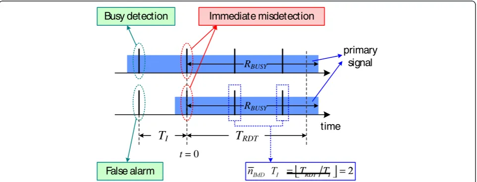
the cases where a secondary user, which has not used the channel due to either the last false alarm or the last busy detection, returns to the channel for spectrum sensing. First, the TDP for the case where the secondary user commits misdetection as soon as it returns to the channel (the so-called immediate misdetection, IMD) is derived. Then, the TDP for the case where the secondary user correctly judges the channel to be idle as soon as it returns to the channel (the so-called CID) is derived.
3.1. IMD
Let the time when IMD occurs be zero (i.e.,t =0) as in Figure 2. Either the false alarm or the correct busy detection can be followed by this IMD. If the residual number of sensing periods overlapped with a primary signal until the primary signal disappears isn(say that a secondary user has n detection opportunities), then the probabilityPd,ithat a secondary user detects the primary signal at itsith detection opportunity is
Pd;i¼ pdð1pdÞ i1;
if 1≤i≤n;
0; otherwiseðn¼i¼0Þ:
ð3Þ
The probability that a secondary user detects the primary signal withinndetection opportunities, Pd(n), is given by
Pdð Þ ¼n
Xn
i¼0Pd;i¼1ð1pdÞn: ð4Þ
In the IMD case, nis dependent on both the residual busy period (denoted byRBUSY) and the sensing interval
Immediate misdetection
primary signal
False alarm
time
RBUSY
TRDT
TI
t= 0
Busy detection
RBUSY
(denoted byTI). From the renewal theory, for a primary
signal’s alternating renewal process, if a primary signal is present at the time t= 0, then the residual busy period
RBUSYhas the pdf form asfRBUSYð Þ ¼x 1
E T½ BUSY. The probability that a secondary user has n detection opportunities withTIcan be given by
PIMDDO ðn;TIÞ ¼PrfRBUSY≥nTIg
PrfRBUSY≥ðnþ1ÞTIg: ð5Þ
Since we are interested in the detection probability within TRDT, the number of detection opportunities is
upper-bounded. This means that, even if the residual busy period of a primary signal is larger than the RDT (i.e., RBUSY > TRDT), the probability that the primary
signal is detected after TRDT does not contribute to
the TDP. The upper-bounded number of detection opportunities for the IMD case can be expressed as a function ofTIas can rewrite (5) as follows
PIMD
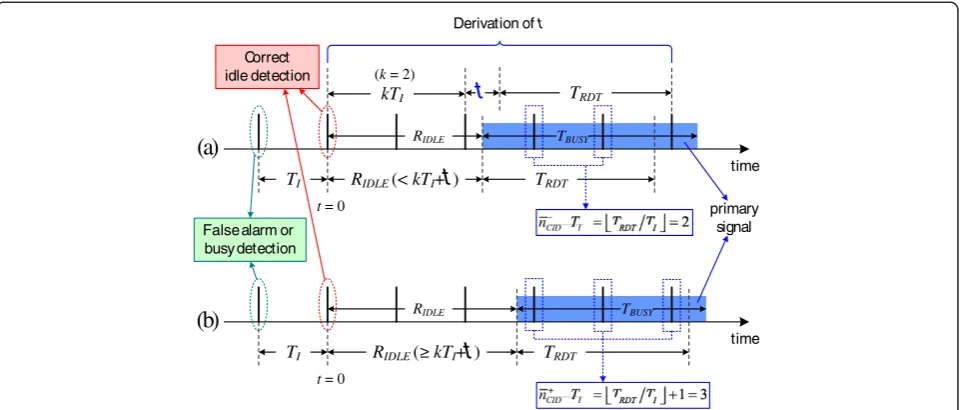
Then, the TDP for the IMD case can be obtained as follows
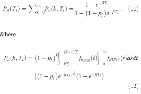
The principle to derive the TDP for the CID case is almost the same as that in the IMD case, but the residual idle periodRIDLE, followed byTBUSY, is additionally
consid-ered. Moreover, the upper-bounded number of detection opportunities for the CID case differs according to the range ofRIDLE. Similar toRBUSY, if a primary signal is not
present at the timet= 0, then the residual idle periodRIDLE
has the pdf form of fRIDLEð Þ ¼x 1
upper-bounded number of detection opportunities for the CID case (denoted by nCIDð ÞTI ). Letkbe an integer denoting the number of sensing intervals fully contained
in RIDLE, i.e., k= ⌊RIDLE/TI⌋(k = 0,1,2. . .) andτbe the
upper-bounded number of detection opportunities is the same as nIMDð ÞTI in (6), but ifkTI+τ≤RIDLE< (k+ 1) TI, one more upper-bounded detection opportunity is
expected, i.e., probability that a secondary user hasndetection oppor-tunities withTIdiffers depending on the range ofRIDLE.
To derive the number of detection opportunities under kTI ≤RIDLE< (k+ 1)TI, it is required that a secondary
user does not commit any false alarms during the fully idle intervals (i.e.,ksensing intervals). This is because, if a false alarm occurs during the ksensing intervals, this situation is considered as either a new CID case or a new IMD case. All the events that a primary signal arrives at the channel during any kth sensing interval occur with the probabilityPA(TI) given as
PAð Þ ¼TI
ondary user has n detection opportunities with TI is
PDOCID n;TI;k;nCIDð ÞTI
in derivation, because they are unavoidable misdetections (i.e., in (3),Pd,0= 0). However, they (negatively) contribute
to the TDP for CID cases since they are treated as the events of interest in (11) and (12).
The TDP for CID cases can be expressed as follows
PCIDD ð Þ ¼TI
XnCIDð ÞTI
n¼1 P
CID
DO n;TI;nCIDð ÞTI
Pdð Þn
þXnþCIDð ÞTI
n¼1 PDOCID n;TI;nþCIDð ÞTI
Pdð Þn:
ð19Þ 3.3. TDP
As aforementioned, we need to consider only the case of D0. However, when a secondary user declares that the
channel is idle, it does not know whether or not its decision is correct. The probability that the channel is busy is P(H1) = β/(α + β) and the probability that the
channel is idle isP(H0) =α/(α+β). From Bayes’theorem
and the law of total probability, the probability that the channel is actually idle when the channel is judged to be idle (i.e., the probability of CID occurrence) can be obtained byP(H0|D0) =P(H0)P(D0|H0)/
P
i∈{0,1}P(Hi)P(D0|Hi), where P(D0|H0) = 1 −pfand P(D0|H1) = 1 − pd. Similarly, the
probability that the channel is actually busy when the channel is judged to be idle (i.e., the probability of IMD occurrence) can be obtained byP(H1|D0) =P(H1)P(D0|H1)/
P
i∈{0,1}P(Hi)P(D0|Hi). Then, the final form of TDP can be
given by
PDð Þ ¼TI PðH1j ÞD0 PIMDD ð Þ þTI PðH0j ÞD0PCIDD ð ÞTI
¼P Hð Þ1ð1pdÞPDIMDð Þ þTI P Hð Þ0 1pf
PCID
D ð ÞTI P Hð Þ1 ð1pdÞ þP Hð Þ0 1pf
:
ð20Þ
4. Sensing parameter optimization
In this section, the sensing parameter optimization problem that maximizes the achievable throughput for the secondary users is presented. Two kinds of constraints for the protection of primary signals are considered: (i) required TDP pD and (ii) required interference ratio. The achievable throughput for secondary users and interference ratio are defined and derived in the following section. We first present the sensing interval optimization problem. Then, the sensing parameter optimization problem determining both the optimal sensing duration and interval is discussed.
4.1. Sensing interval optimization problem
When energy detection is used for a secondary user’s sensing method, the sensing durationTScan be expressed as a function of two variables, PSDPpdand PSFAPpf, as follows [3]
TS pd;pf
¼ 1
fs⋅γ2
Q1 pf Q1ð Þpd
ffiffiffiffiffiffiffiffiffiffiffiffiffiffi
2γþ1
p
2
;
ð21Þ
where fs is the sampling frequency,γ the target received signal-to-noise ratio (SNR) at the secondary user, andQ(∙) is theQ-function. Hereafter, the termTSis used instead of TS(pd,pf) for simplicity. To focus on the sensing interval optimization problem, we assume that pd and pf (and thus TS) are given. While considering the periodic sensing, once a secondary user judges the channel to be idle (i.e.,D0) duringTS, it utilizes the channel until
the next sensing duration (i.e., during TI – TS). We
assume that, during the secondary user’s transmission, the fraction of busy periods does not contribute to the throughput for both secondary and primary users due to the mutual interference. Then, the achievable throughput for secondary users can be defined as the expected fraction of idle periods under D0. Given the pdandpf, it can be expressed as a function of a sensing interval, denoted by R(TI). Similarly, the interference ratio can be defined as the expected fraction of busy periods interrupted by the secondary user’s transmission and expressed as a function of a sensing interval, denoted by I(TI). Then, our sensing interval optimization problem
can be expressed as follows
FindTIthat maximizeR Tð ÞI ; subject toPDð Þ≥TI PD
andI Tð Þ≤I I;
ð22Þ
where TI* is the optimal sensing interval and I is the required interference ratio given by primary network as in [10]. Since the exponential busy and idle periods with rate parametersαandβare assumed,R(TI) andI(TI) can easily
be obtained by using the renewal theory. If the judgment D0is correct (i.e.,D0|H0) at timet0, then the expected time
during which the channel is idle during the time betweent0
andt0+tcan be given by [14,15]
δIDLE
D0jH0ð Þ ¼t tP Hð Þ1 Δð Þt ;
ð23Þ
where Δ(t) = t + {e−(α+β)t − 1}(α + β)−1. Similarly, the expected idle time after misdetection (i.e., D0|H1) during
the upcomingttime is given by
δIDLE
D0jH1ð Þ ¼t P Hð Þ0 Δð Þt :
ð24Þ
R Tð Þ ¼I
On the other hand, from (23) and (24), the expected time during which the channel is busy during the time be-tweent0andt0+tis obtained byδBUSYD0jH0ð Þ ¼t tδ
misdetection, respectively. Then, from the definition, I(TI)
can be given by
It should be noted that,pd>pfis generally considered in CR networks (i.e.,pdcloser to one andpfcloser to zero for efficient primary protection and spectrum utilization are desired). Then, for any givenpdandpf,I(TI) is a
monoton-ically increasing function ofTI, since (i)Δt) is an increasing
function oftand (ii) obviously,TI>TS. Thus, there exists a
maximum affordable sensing interval for the interference ratio constraint, denoted by maxTIIR, such that I Tð Þ ¼I I. Moreover, as discussed in Section 3, for any givenpdandpf PD(TI) is a monotonically decreasing function ofTI.
There-fore, there is a maximum affordable sensing interval for the TDP constraint, denoted by maxTITDP,, such that PDð Þ ¼TI PD. Basically, these facts implies that the opti-mal sensing intervalTI*should be found within the range (TS, min(maxTIIR, maxTITDP)]. On the other hand, R(TI)
can be either a concave function or a monotonically
increasing function of TI, i.e., if pdpf
wise, a monotonically increasing function ofTI(the proof is
omitted in this article). Thus, if R(TI) is a monotonically
increasing function of TI, TI* = min{maxTIIR, maxTITDP},
and otherwise, TI* = min{ TImaxTH, maxTIIR, maxTITDP},
whereTImaxTHis the sensing interval that maximizesR(TI).
From the above discussion, we can say that, for any given pdand pf, there exists the one and only oneTI* that yields the maximum achievable throughput under the two con-straints, which can be obtained by 1D exhaustive search.
4.2. Sensing duration and interval optimization problem PD(TI), R(TI), and I(TI) are commonly affected by not
onlyTI, but also the parameterspdandpf. This implies that,
PD(TI),R(TI), andI(TI) can be expressed as functions of the
three parameters, i.e.,PD(pd,pf,TI),R(pd,pf,TI), andI(pd,pf,TI).
Obviously, any change inpdorpfresults in differentTSby (21), maxTIIR, and maxTITDP, and finally differentTI*andR (pd,pf,TI*). From this, the problem in (22) can be extended to the sensing duration and interval optimization problem as follows
Since the existence of optimal sensing interval TI* for any given pd and pf is proved in the previous section, it can be expected that, the one and only one pair of optimal sensing parameter and interval, denoted by TSOPTandTIOPT, can be found by using the 3D exhaustive
search with the three parameters,pd,pf, andTI.
5. Performance evaluation
In this section, we provide the numerical results related to the TDP. In every experiment, energy detection is consid-ered as the sensing method with sampling frequencyfs= 6 MHz and SNRγ=–15 dB. When the sensing accuracy of a secondary user (e.g., PSDP and PSFAP) is provided, the sensing durationTIcan be obtained by using (21). We first
show the effect of the sensing interval on the TDP. Then, the performance related to the sensing parameter optimization is presented in detail. The required TDP of 0.9 (i.e., PD¼0:9 ) and the required interference ratio of 0.1 (i.e., I¼0:1 ) are used as the constraints for primary user protection.
5.1. Effect of sensing interval on TDP
Figure 4 shows the TDP, PD(TI), explained in Section 3
in accordance with the sensing interval TI, for different
{α,β} pairs, whilepd= 0.9 andpf= 0.1 are used.TRDTis
set to be 2 s. First of all, it should be noted that when the required PSDP of 0.9 (i.e.,pd¼0:9) is solely considered as the constraint for primary user protection as in [3-5], it is believed that regardless of the length of sensing interval, all primary users in Figure 4 are sufficiently protected sincepd= 0.9 is used. In this case, however, the unavoidable misdetections and lengthy detection latency problems are not considered at all. On the contrary, our TDP considers these problems naturally and provides a maximum afford-able sensing interval based on the givenPD. In Figure 4, as expected, the TDP is a decreasing function of TI. The
intersection point between the TDP curve for each {α,β} pair and the line of the required TDP is maxTITDP. If the
required TDP larger than 0.9 is applied, the smaller max TITDPis expected. We can observe that every curve sharply
decrement of the upper-bounded number of detection opportunities in (6) and (10). When the channel state frequently changes (i.e., whenαandβare relatively large), a relatively small maxTITDP is obtained. In this case,
unavoidable misdetections are the main factors reducing the maxTITDP. On the other hand, when the channel state
infrequently changes, unavoidable misdetections are less considered and the maxTITDP is mainly affected by the
detection latency underTRDT. Hence, whenTRDTis fixed,
maxTITDP grows as α and β decrease. However, even
thoughαandβare very small, maxTITDPcannot exceed a
certain value. It can easily be understood by the example where pd¼PD as in Figure 4. In this example, maxTITDP
cannot exceedTRDTeven with very smallαandβ, because
the probability of an unavoidable misdetection is always larger than zero.
In this experiment, when α = 0.5, the mean busy period is 2 s. In this case, the RDT of 2 s is very large compared to the mean busy period of 2 s, which may be not desired by primary users due to the less protection degree (i.e., primary signals are expected to suffer from lots of unavoidable misdetections and lengthy detection latency). For this reason,TRDT = 0.1 × E[TBUSY] is used
in the rest of this section.
5.2. Optimal sensing interval with givenpdandpf
In this section, our optimal sensing intervalTI*in (22) is evaluated and compared with the conventional optimal sensing interval, under the condition that pdand pf are given. The conventional optimal sensing interval is derived by using the approach in [10], where the interference ratio constraint is solely used for primary user protection. On the other hand, the proposed optimal sensing interval uses both the interference ratio and TDP constraints. As the given values for sensing accuracy, any pd satisfying the condition pd≥ð1IÞ is used whilepfis fixed to 0.1. The condition forpdcomes from (26). The second term in (26)
is relatively small compared to the first term and always larger than zero. Besides, for the first term in (26),TS is usually very small compared to TI. Then, the dominant
factor of the interference ratio is (1−pd), and thus we only considerpd≥ð1IÞ.
First, Figure 5 shows that, according to the circum-stances, any of the three sensing intervals, maxTITDP,
maxTIIR, andTImaxTH [in Figure 5, every set satisfies the condition for R(TI) to be a concave function ofTI], can
be selected as the optimal sensing interval TI*. In each curve, the empty circle ‘o’, the empty triangle ‘Δ’, and the colored square ‘■’ represent maxTITDP, maxTIIR,
and TImaxTH, respectively. For dashed lines, maxTITDP≈
0.199 ms, maxTIIR≈0.251 ms, andTImaxTH≈0.263 ms, and 0.2
0.3 0.4 0.5 0.6 0.7 0.8 0.9 1
0 0.5 1 1.5 2 2.5 3
TI (s)
TD
P
, P
D
(T
I
)
required TDP
p = 0.9 p = 0.1 maxTTDP
0.321s I
maxTTDPI 1.889s
maxTITDP 1.372s
Figure 4TDP as a function ofTI, wherepd= 0.9 andpf= 0.1.
Figure 5Optimal sensing intervals selected for different environments: the lines with‘o’,‘Δ’, and‘■’represent the performance of TDP, interference ratio, and achievable throughput, respectively.
thusTI*for dashed lines isTI*= min{TImaxTH, maxTIIR, max TITDP}. Similarly, the optimal sensing intervals for solid
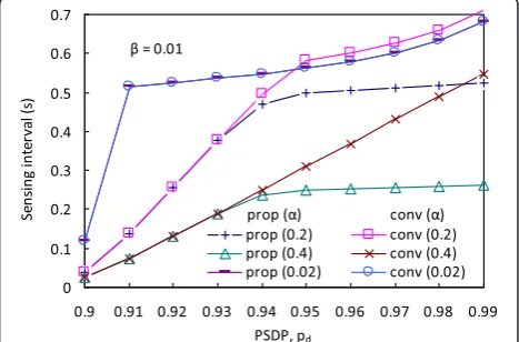
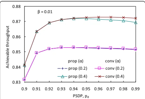
and dotted lines are maxTIIRandTImaxTH, respectively. Figure 6 shows the comparison between the proposed optimal sensing interval and the conventional optimal sensing interval for different (pd, pf) combinations. The TDP, achievable throughput, and interference ratio performances by those selected sensing intervals are shown in Figures 7, 8, and 9, respectively. In these experiments,
βis fixed to 0.01. In Figure 6, basically, we can see that the optimal sensing interval increases as the PSDP increases in both the proposed and conventional cases. This can be understood based on the relationships between the sensing interval and the performance metrics: (i) the larger PSDP yields the lower interference ratio, and thus the larger max TIIR, (ii) the larger PSDP yields the larger maxTITDP. In
Figure 6, when the primary signal infrequently changes its state (i.e., bothαandβare relatively small:α= 0.02 in the experiment), the proposed optimal sensing interval is the same with the conventional one. This means that those
sensing intervals commonly satisfy the TDP constraint in (2). However, when the primary signal infrequently occurs with a relatively short busy period compared to the idle period (i.e.,α is noticeably larger thanβ: α= 0.2 or 0.4 in the experiment), the proposed optimal sensing interval is smaller than the conventional one while the given pd is larger than or equal to 0.94 (it should be noted that the condition whereα is noticeably larger than βis the most desirable situation in CR networks, since the spectrum efficiency is remarkably low). This is due to the adoption of TDP constraint as shown in Figure 7. Figure 7 shows that the proposed optimal sensing interval satisfies the TDP constraint for any givenpd, while the conventional optimal sensing interval does not whenpd≥0.94. This means that the conventional optimal sensing interval may cause the unavoidable misdetections and lengthy detection latency more than the primary system’s tolerable limit. This problem becomes more critical as the PSDP or α grows. On the contrary, our approach effectively mitigates this problem by maintaining the sensing interval not to cause the TDP exceeding the required one. Due to the reduced optimal sensing interval, the achievable throughput for the proposed approach can be reduced, but is not significantly different compared to that for the conventional approach as shown in Figure 8. Moreover, as a result of the reduced sensing interval, the proposed optimal sensing interval may further reduce the interference ratio than the conventional one as shown in Figure 9.
5.3. Optimal sensing duration and interval
Let us focus on the case where α= 0.4 and β= 0.01 in Figure 8. With the proposed optimization problem in (27), for the given PSFAP of 0.1, the achievable throughput can be maximized by selecting the PSDP of 0.94 among others. In this case, the sensing duration is about 1.387 ms from (21) and the sensing interval is about 0.235 s as shown in Figure 6. These are not the global optimal sensing
Figure 7TDP performances associated with selected sensing intervals.
Figure 8Achievable throughput performances associated with selected sensing intervals.
parameters, because only the PSFAP of 0.1 has been considered in Figure 8. To find the global optimal sensing parameters for the proposed approach (TSOPTand T1OPT),
the more results with different PSFAP should be obtained and compared with each other. By comparing the results obtained for different PSFAPs (PSFAP decreases by 0.01 per experiment), the maximum achievable throughput is obtained when TI = 0.25 s and TS = 2.697 ms corre-sponding to (pd,pf) = (0.95,0.01). These sensing interval and duration are the global optimal sensing parameters (i.e.,TSOPT = 2.697 ms andT1OPT = 0.25 s) for the case
whereα= 0.4 andβ= 0.01. The global optimal sensing duration and interval for the conventional approach can be found in a similar way. Either very small PSFAP (e.g., 0.001) or very large PSDP (e.g., 0.999) could be considered, but we did not consider such values, since the sensing duration would be non-negligible (i.e., the probability that a primary signal may appear or disappear during the sensing duration is non-negligible). In the following experiments, pf∈{0.01, 0.02,⋯, 0.1} and pd∈ {0.9, 0.91,⋯, 0.99} are used to find the global optimal sens-ing parameters (the maximum senssens-ing duration with the
givenpfandpdis 3.721 ms wherepf= 0.01 andpd= 0.99).
αfrom 0.1 to 1 and a fixedβof 0.01 are used in the experi-ments, which reflects the low spectrum efficiency.
In Figure 10, bothTSOPTand T1OPTare relatively small
compared to the optimal sensing duration and interval for the conventional approach, except for the case where
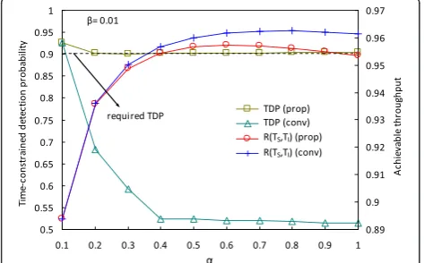
α= 0.1. The TDP and the achievable throughput corre-sponding to the optimal sensing parameters are also investigated in Figure 11. Similar to the results in the previous section, we can see that the achievable throughput for the proposed approach (withTSOPTandT1OPT) is slightly
smaller than that for the conventional approach, while satisfying the TDP constraint. On the other hand, the optimal sensing duration and interval for the conventional approach significantly violate the TDP constraint. Figure 12 additionally shows that the interference ratio can be further reduced with TSOPT and T1OPT, which implies that our
proposed approach can protect primary signals better than the conventional approach. From Figures 11 and 12, we can also see that, as α grows (as the spectrum efficiency decreases), the proposed approach with TDP constraint
Figure 10Optimal sensing duration and interval obtained by the proposed and conventional optimization problems.
Figure 11TDP and achievable throughput associated with optimal sensing parameters.
Figure 12Interference ratio associated with optimal sensing parameters.
1 1.5 2 2.5 3 3.5 4 4.5 5
0.1 0.2 0.3 0.4 0.5 0.6 0.7 0.8 0.9 1
O
p
ti
m
a
l s
e
n
s
in
g
d
u
ra
tio
n
(m
s
)
0 0.1 0.2 0.3 0.4 0.5 0.6 0.7 0.8 0.9
O
p
ti
m
a
l s
e
n
s
in
g
in
te
rv
a
l (s
)
opt Ts (0.9, 0.1) opt Ts(0.95, 0.1) opt Ts(0.9, 0.05)
Ti(0.9, 0.1) Ti(0.95, 0.1) Ti(0.9, 0.05)
β=0.01
opt.TS (0.9,0.1) opt .TS (0.95,0.1) opt.TS (0.9,0.05)
opt.TI (0.9,0.1) opt.TI (0.95,0.1) opt.TI (0.9,0.05)
( PD, I )
_ _
opt.TS & opt.TI( PD, I )
_ _
outperforms the conventional approach in terms of TDP and interference ratio, at the cost of slightly re-duced throughput.
Figure 13 shows the optimal sensing parameters for different TDP and interference ratio constraints. When the constraints with either the largerPD or the smallerI is applied, primary signals are supposed to be more protected. In this situation, at least either the larger pd or the smaller sensing interval is generally required. The results withPD = 0.9 andI = 0.1 are used as a reference to others. When the smallerI is applied,TSOPTincreases
andT1OPTdecreases. One of the key factors that increase T1OPTis the larger lower-boundedpddue to the smallerI (i.e.,pd≥1I). On the other hand, when the largerPDis applied, bothTSOPTandT1OPTdecrease.
6. Conclusions
In this article, we have introduced and defined a new detection probability, of the so-called TDP, by taking both the detection latency and unavoidable misdetection into account. The new detection probability is also derived as a function of a sensing interval. The sensing parameter optimization problem is also discussed while the achievable throughput, interference ratio, and their respective characteristics in the view point of the sensing interval are investigated in detail. The sufficient protection of primary signals can be achieved by the proposed optimal sensing parameters, which are especially satisfying to the TDP constraint, but not by the optimal sensing parameters focusing only on the PSDP or the interference ratio constraint. Even though the achievable throughput with the proposed optimal sensing parameters can be smaller than that with the conventional optimal sensing parameters, the difference is not significant. The appli-cation of the TDP constraint is required to sufficiently protect primary signals and more significantly when the spectrum efficiency is low.
Competing interests
The authors declare that they have no competing interests.
Acknowledgments
This study was supported by the Basic Science Research Program through the National Research Foundation of Korea (NRF) funded by the Ministry of Education, Science and Technology (No. 2011-0021152).
Received: 12 July 2012 Accepted: 11 December 2012 Published: 21 January 2013
References
1. FCC,Spectrum policy task force report. FCC 02155(2002)
2. J Mitola, Cognitive radio for flexible mobile multimedia communications, inProceedings of the IEEE International Workshop on Mobile Multimedia Communications (MoMuC 1999)(San Diego, California), pp. 3–10. November 1999
3. YC Liang, Y Zeng, ECY Peh, AT Hoang, Sensing-throughput tradeoff for cognitive radio networks. IEEE Trans. Wirel. Commun.7(4), 1326–1337 (2008)
4. ECY Peh, YC Liang, YL Guan, Y Zeng, Optimization of cooperative sensing in cognitive radio networks: a sensing-throughput tradeoff view. IEEE Trans. Veh. Technol.58(9), 5294–5299 (2009)
5. R Fan, H Jiang, Optimal multi-channel cooperative sensing in cognitive radio networks. IEEE Trans. Wirel. Commun.9(3), 1128–1138 (2010) 6. Y Pei, AT Hoang, YC Liang, Sensing-throughput tradeoff in cognitive radio
networks: how frequently should spectrum sensing be carried out? in Proceedings of the IEEE International Symposium on Personal, Indoor and Mobile Radio Communications (PIMRC 2007)(Athens, Greece), pp. 1–5. September 2007
7. D Xue, X Wang, E Hossain, Optimization of periodic channel sensing by secondary users in a cognitive radio network, inProceedings of the IEEE Global Communications Conference (Globecom 2010)(Miami, Florida), pp. 1–5. December 2010
8. H Du, Z Wei, L Ye, Y Wang, D Yang, Transmitting-collision tradeoff in cognitive radio networks: a flexible transmitting approach, inProceedings of the International ICST Conference on Cognitive Radio Oriented Wireless Networks and Communications (CrownCom 2011)(Osaka, Japan), pp. 271–275. June 2011 9. S Zarrin, TJ Lim, Throughput-sensing tradeoff of cognitive radio networks
based on quickest sensing, inProceedings of the IEEE International Conference on Communications (ICC 2011)(Kyoto, Japan), pp. 1–5. June 2011 10. WY Lee, IF Akyildiz, Optimal spectrum sensing framework for cognitive radio
networks. IEEE Trans. Wirel. Commun.7(10), 3845–3857 (2008) 11. IEEE Std 802.22-2011, IEEE Standard for Information
Technology-Telecommunications and Information Exchange between Systems Wireless Regional Area Networks (WRAN)-Specific Requirements Part 22: Cognitive Wireless RAN Medium Access Control (MAC) and Physical Layer (PHY) Specifications: Policies and Procedures for Operation in the TV Bands(2011) 12. C Cordeiro, M Ghosh, D Cavalcanti, K Challapali, Spectrum sensing for
dynamic spectrum access of TV bands, inProceedings of the International ICST Conference on Cognitive Radio Oriented Wireless Networks and Communications (CrownCom 2007)(Orlando, Florida), pp. 225–233. July-August 2007 13. H Kim, KG Shin, In-band spectrum sensing in cognitive radio networks:
energy detection or feature detection? inProceedings of the International Conference on Mobile Computing and Networking (ACM MobiCom 2008) (San Francisco, California), pp. 14–25. September 2008
14. H Kim, K Shin, Efficient discovery of spectrum opportunities with MAC-layer sensing in cognitive radio networks. IEEE Trans. Mob. Comput.
7(5), 533–545 (2008)
15. DR Cox,Renewal Theory(Butler and Tanner, London, UK, 1967)
doi:10.1186/1687-1499-2013-9
Cite this article as:Choi and Yoo:Time-constrained detection probability and sensing parameter optimization in cognitive radio networks.EURASIP Journal on Wireless Communications and Networking
20132013:9.
Submit your manuscript to a
journal and benefi t from:
7Convenient online submission 7Rigorous peer review
7Immediate publication on acceptance 7Open access: articles freely available online 7High visibility within the fi eld
7Retaining the copyright to your article