R E S E A R C H
Open Access
Structured optimal transmission control in
network-coded two-way relay channels
Ni Ding
*, Parastoo Sadeghi and Rodney A. Kennedy
Abstract
This paper considers a transmission control problem in network-coded two-way relay channels (NC-TWRC), where the relay buffers randomly arrived packets from two users, and the channels are assumed to be fading. The problem is modeled by a discounted infinite horizon Markov decision process (MDP). The objective is to find an adaptive
transmission control policy that minimizes the packet delay, buffer overflow, transmission power consumption and downlink error rate simultaneously and in the long run. By using the concepts of submodularity, multimodularity and
L-convexity, we study the structure of the optimal policy searched by dynamic programming (DP) algorithm. We show that the optimal transmission policy is nondecreasing in queue occupancies and/or channel states under certain conditions such as the chosen values of parameters in the MDP model, channel modeling method, and the preservation of stochastic dominance in the transitions of system states. Based one these results, we propose to use two low-complexity algorithms for searching the optimal monotonic policy: monotonic policy iteration (MPI) and discrete simultaneous perturbation stochastic approximation (DSPSA). We show that MPI reduces the time complexity of DP, and DSPSA is able to adaptively track the optimal policy when the statistics of the packet arrival processes change with time.
Keywords: Cross-layer optimization, Discounted Markov decision process, Discrete stochastic approximation, Dynamic programming,L,-convexity, Multimodularity, Network coding, Submodularity
1 Introduction
Network coding (NC) was proposed in [1] to maxi-mize the information flow in a wired network. It was introduced in multicast wireless communications to opti-mize the throughput and has attracted significant interest recently due to the rapid growth in multimedia applica-tions [2]. It was shown in [3] that the power efficiency in wireless transmission systems could be improved by NC. For example, in a 3-node network system, called the network-coded two-way relay channels (NC-TWRC) [4] as shown in Fig. 1, the messagesm1andm2are XORed at the relay and broadcast to the end users. This method, compared to the conventional store-and-forward trans-mission, reduces the total number of transmissions from 4 to 3 so that the transmission power is saved by 25 %. Since then, numerous optimization problems have been studied in NC-TWRC, e.g., the precoding scheme design
*Correspondence: [email protected]
Research School of Engineering, College of Engineering and Computer Science, Australian National University (ANU), 2601 Canberra, Australia
proposed in [5], the optimal achievable sum-rate prob-lem studied in [6] and the optimal beamforming method proposed in [7].
In [8], Katti et al. pointed out the importance of being opportunistic in practical NC scenarios. It was suggested that the assumptions in the related research work should comply with the practical wireless environments, e.g., decentralized routing and time-varying traffic rate. This suggestion highlighted a problem in the existing literature; the majority of the studies (e.g., [9, 10]) consider static environments (e.g, synchronized traffic) while ignoring the stochastic nature of the packet arrivals in the data link layer. On the other hand, the randomness of traffic in Fig. 1 poses the problem of how to make an optimal decision in a dynamic environment with a power-delay tradeof;: when there are packet inflows in the relay but no coding opportunities or XORing pairs (e.g., one packet arrives from one user, but no packet arrives from the other), waiting for coding opportunities by holding pack-ets saves transmission power but increases packet delay and results in more packets to be transmitted in the
Fig. 1NC-TWRC [4]. Two users exchange information (m1andm2) via the center nodeR(stands for relay)
future. Since a decision made at any instant affects both the immediate and future costs, the decision-making is a dynamic, instead of a one-time, process, i.e., the objec-tive is to determine a decision rule that is optimal over time. In [11, 12], this problem was studied and solved by a cross-layer design, NC-TWRC with buffering. The opti-mal policy by Markovian process formulation was shown to minimize the transmission power and packet delay simultaneously and in the long run. In [13], the buffer-assisted NC-TWRC was extended to include the dynamics of wireless channels (Fig. 2). In this system, a transmission policy that solves power-delay tradeoff may not be the best decision rule because it does not consider the possible loss in throughput due to the downlink transmission errors. For this reason, the scheduler is required to make an optimal decision that simultaneously minimizes the trans-mission power, packet delay, downlink BER in the long run by considering current queue and channel states and their expectations in the future. In [13], this problem was for-mulated by a discounted infinite horizon Markov decision process (MDP) [14] with channels modeled by finite-state Markov chains (FSMCs) [15]. The optimal transmission policy was shown to be superior to [11, 12] in terms of enhancing the QoS (quality of service, evaluated by packet delay and overflow in the data link layer, and power con-sumption and error rate in the physical layer) in a practical wireless environment, e.g., Rayleigh fading channels.
The optimal policy of a discounted infinite horizon MDP can be found by dynamic programming (DP) [16], value or policy iterations. However, the DP algorithm is burdened with high complexity. In Fig. 2, the sys-tem state is a 4-tuple (two channels and two queues), and the decision/action is a 2-tuple (each associated with the departure control of one queue). In such a high
dimensional MDP, the curse of dimensionality1becomes more evident [17]; the computation load grows quickly if the cardinality of any tuple in the state variable is large. To relieve the curse, one solution is to qualitatively under-stand the model and prove the existence of a monotonic optimal policy [18]. Then, a low complexity algorithm or a model-free learning method can be proposed, e.g., simul-taneous perturbation stochastic approximation (SPSA) [19, 20]. But, monotonic optimal policy does not exist in general. Most often, optimal policy exists, but it varies with the state variable irregularly. In order to prove the existence of certain feature in the optimal policy, we need to extensively analyze the MDP model and the recur-sive functions in DP algorithm. The basic approach in the existing literature is to show by induction that the submodularity is preserved in each iterative optimization process (maximization/minimization) in DP, e.g., [19, 21]. We adopt the same method in this paper but consider a submodularity in high dimensional cases. Moreover, we useL-convexity and multimodularity, two concepts that were originally defined in discrete convex analysis [22, 23], to describe the joint submodularity and integral convexity in a high dimensional space.
The aim of our work is to prove the existence of a monotonic optimal transmission policy in the NC-TWRC system in Fig. 2. By observing theL-convexity and sub-modularity of DP function, we derive the sufficient condi-tions for the optimal policy to be nondecreasing in queue and/or channel states. These structured results are used to derive two low complexity algorithms: monotonic policy iteration (MPI) and discrete simultaneous perturbation stochastic approximation (DSPSA). We compare the time complexity of MPI to that of DP and show the convergence performance of DSPSA algorithm. The main results in this paper are:
• We prove that each tuple in the optimal policy is nondecreasing in the queue state that is controlled by that tuple if the chosen values of unit costs in immediate cost function give rise to anL-convex or multimodular DP. Moreover, we show that the same results found in [19, 21] can also be explained by
L-convexity or multimodularity by a unimodular coordinate transform.
• By thinking of each iteration in DP as a one-stage pure coordination supermodular game, we show that equiprobable traffic rates and certain conditions on unit costs guarantee that each tuple in the optimal policy is monotonic in not only the queue state that is controlled by that tuple but also the queue state that is associated with the information flow of the opposite direction, i.e., the one that is not under the control of that tuple.
• By observing the submodularity of DP, we show the sufficient conditions for an optimal policy to be nondecreasing in both queue and channel states in terms of unit costs, channel statistics, and FSMC models.
• Based on the submodularity, multimodularity, and L-convexity of DP, we show that the optimal transmission control problem in Fig. 2 can be solved by two low-complexity algorithms. One is MPI, a modified DP algorithm with the action searching space progressively shrinking with the increasing indices of queue and/or channel states. It is shown that the time complexity of MPI is much less than that of DP when the cardinality of system state is large. The other algorithm is a stochastic optimization method. We formulate the optimal policy searching problem by a minimization problem over a set of queue thresholds and use the DSPSA algorithm to approximate the minimizer. We show that DSPSA is able to adaptively track the optimal values of queue thresholds when the statistics of packet arrival processes change with time. We run simulations in NC-TWRC with Rayleigh fading channels to show that the average cost incurred by the policy approximated by DSPSA is similar to that incurred by the optimal policy searched by DP.
The rest of this paper is organized as follows. In Section 2, we state the optimization problem in NC-TWRC with random packet arrivals and FSMC modeled channels and clarify the assumptions. In Section 3, we describe the MDP formulation, state the objective, and present the DP algorithm. In Section 4, we investigate the structure in the optimal transmission policy found by DP algorithm in queue and channel states. Section 5 presents MPI and DPSA algorithms.
2 System
Consider the NC-TWRC shown in Fig. 2. User 1 and 2 randomly send packets to each other via the relay. The relay is equipped with two finite-length FIFO queues, queue 1 and 2, to buffer the incoming packets from user 1 and 2, respectively. The outflows of queues are
controlled by a scheduler. The scheduler keeps making decisions as to whether or not to transmit packets from queues. If the decision results in a pair of packets in oppo-site directions transmitted at the same time, they will be XORed (coded) and broadcast. Otherwise, the packet will be simply forwarded to the end user. The objective is to minimize packet delay, queue overflow, transmission power (saved by utilizing the coding opportunities), and downlink transmission errors simultaneously and their expectations in the future. Obviously, the optimization concerns are contradictory to each other: (1) If there does not exist a pair of packets for XORing, waiting for coding opportunity by holding packets results in a high packet delay on average, while transmitting a packet without cod-ing results in one more packet to be transmitted in the future, i.e., more transmission power on average; (2) If the SNR of one channel is low, waiting for high SNR tran-sition by holding packets results in higher packet delay but lower transmission error rate. Therefore, the sched-uler must seek an optimal decision rule that solves this power-delay-error tradeoff.
It should be pointed out that the problem under consid-eration is a cross-layer multi-objective optimization one; we want to optimize both the power consumption and transmission error rate in the physical layer and the packet delay in the data link layer. As discussed above, since there are tradeoffs among these optimization metrics, it is not possible to get all of them optimized simultaneously. Therefore, in this paper, we are actually seeking the Pareto optimality of these optimization metrics.2
2.1 Assumptions
We consider a discrete-time decision-making process, where the time is divided into small intervals, called deci-sion epochsand denoted byt∈ {0, 1,. . .,T}. Leti∈ {1, 2} and assume the following:
A1 (i.i.d. incoming traffic) Denote random variable fi(t)∈Fias the number of incoming packets to queue i at decision epoch t. Let the maximum number of packets arrived per decision epoch be no greater than 1, i.e.,Fi= {0, 1}. Assume that two independenti.i.d. random processes with Prfi(t)=1=piandPr
fi(t)=0=1−pifor allt. A2 (modulation scheme) Packets are of equal length.
A3 (finite-length queues) Queuei can store maximum Lipackets. At eacht, the scheduler makes a decision and incurs an immediate cost before the event
f(t)=
f1(t),f2(t). Denoteb(it)∈Bias the occupancy of queuei at the beginning of decision epoch t, then Bi= queue occupationLi+1, the newly arrived packet will be dropped. We call it packet lost due to the queue overflow.
A4 (Markovian channel modeling) Let the full variation range ofγi(t), the instantaneous SNR of channeli, be partitioned intoKinon-overlapping regions
{[1,2), [2,3),. . ., [Ki,∞)}, called channel
states. Here, the SNR boundaries satisfy
1< 2< . . . < Ki. DenoteGi= {1, 2,. . .,Ki}as
the state set of channeli andgi(t)as the state of channeli at decision epoch t. We say thatgi(t)=kiif
γ(t)
i ∈[ki,ki+1). Each channel is modeled by a
finite-state Markov chain (FSMC) [15], where the state evolution of channeli is governed by the transition probabilityPg(t)
i g( t+1) i =Pr
gi(t+1) |gi(t).
A5 (downlink channel state information) Letg1(t)and
g(2t)be two independent andi.i.d. random processes. The relay has the channel state information (the value of channel state and its transition probabilities) of both channels before the decision making att.
3 Markov decision process formulation
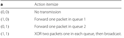
Based on A1, A4, and A5, we know that the statistics of the incoming traffic flow and channel dynamics associ-ated with user 1 or 2 are time-invariant. It follows that the transmission control problem in Fig. 2 can be formu-lated as a stationary Markov decision process (MDP). In the following context, we drop the decision epoch nota-tion t in A1-A5 and use the notation y and y for the system variableyat the current and next decision epochs, respectively. denotes the number of packets departed from queueiand A = A1×A2 = {0, 1}2. The terminology of actions are
(1, 1) XOR two packets one in each queue, then broadcast.
3.3 State transition probabilities The transition probabilityPa
xx = Pr(x|x,a)denotes the probability of being in statex at next decision epoch if actionais taken in statexat current decision epoch. Due to the assumptions of independent random processes in A1 and A5, the state transition probability is given by
Paxx =PabbPgg =
i is determined by channel statistics and FSMC
modeling method in A4 andPai
bibiis the queue state
transi-tion probability. At current decision epoch, the occupancy of queueiafter decisionaiis min{[bi−ai]+,Li}, where [y]+= max{y, 0}. The occupancy at the beginning of the next decision epoch is given by
bi=min[bi−ai]+,Li
+ fi. (2)
Therefore, the state transition probability of queueiis
Pai
where I{·} is the indicator function that returns 1 if the expression in{·}is true and 0 otherwise.
3.4 Immediate cost
C : X×A→ R+is the cost incurred immediately after actiona is taken in statexat current decision epoch. It reflects three optimization concerns: the packet delay and queue overflow, the transmission power, and the downlink transmission error rate.
3.4.1 Holding and overflow cost
We definehi, the holding and queue overflow cost associ-ated with queuei, as
hi(yi)=λmin{[yi]+,Li} +ξoI{[yi]+=Li+1}
=λ[yi]++(ξo−λ)I{[yi]+=Li+1}. (4)
min{[yi]+,Li}andI{[yi]+=Li+1}count the number of
pack-ets held in queue i and the number of packets lost due the overflow of queuei, respectively. We say that the term λmin{[yi]+,Li}accounts for the packet delay because by Little’s Law, the average packet delay is proportional to the average number of packets held in the queue in the long run for a given packet arrival rate [24]. We sum uphifor i∈ {1, 2}and obtain the total holding and overflow cost as
Since forwarding and broadcasting one packet, either coded or non-coded, consume the same amount of energy, we have the immediate transmission cost as
tr(a)=τI{a1=1 ora2=1}=
0 a=(0, 0)
τ otherwise , (6)
where τ > λ is the unit transmission cost and I{a1=1 ora2=1}counts the number of transmissions
result-ing from actiona.
Note that (5) and (6) form a power-delay tradeoff. A policy that always transmits whenever there is an incom-ing packet without considerincom-ing codincom-ing opportunities in the long run is penalized by (6), and a policy that always holds packet to wait for coding opportunities without considering the average packet delay is penalized by (5).
3.4.3 Packet error cost
Since packet errors in downlink transmissions happen only when we decide to transmit, we define the immediate packet error cost due to the actionaias
err(g−i,ai)=ηaiPe(g−i), (7)
whereηis the unit packet error cost and−i∈ {1, 2} \ {i}, i.e.,−i = 2 ifi = 1, and−i = 1 ifi = 2. The reason we have err(g−i,ai)is because the packet departing queueiis transmitted through channel−i, e.g., the relay sends one packet in queue 1 through fading channel 2 whena1=1.
Pe(gi)is estimation of the average BER when transmitting a packet, either coded or non-coded, through channeli when the state isgi. Since BPSK modulation is used at the relay, we definePeas
Note, the aforementioned power-delay tradeoff formed by (5) and (6) just poses the problem of whether or not to transmit if an instantaneous packet inflow is not able to form an XORing pair. However, if the scheduler consid-ers downlink transmission error rate in addition, a policy that always broadcasts XORed packets whenever there is
a coding opportunity without considering downlink chan-nel states is penalized by (7). Therefore, (5), (6), and (7) form a power-delay-error tradeoff.
In summary, we define the immediate cost as
C(x,a)=C(b,g,a)=Ch(b,a)+Ct(g,a), (9) tions (each quantifies an optimization concern). The unit costλ,ξo,τ, andηcan be considered as the weight fac-tors that are either given or adjustable depending on the real applications. In Section 4, we will derive the sufficient conditions of the existence of a structured optimal policy mainly in terms of the chosen values of these unit costs.
3.5 Objective and dynamic programming
Letx(t) and a(t) denote the state and action at decision epoch t, respectively, and consider an infinite-horizon MDP modeling where the discrete decision making pro-cess is assumed to be infinitely long. We can describe the long-run objective as counted factor that ensures the convergence of the series. It is proved in [14] that if the state spaceX is countable, the action setAis finite, and the MDP is stationary, there exists a deterministic stationary policyθ∗ : X →Athat optimizes (11), andθ∗can be searched by DP
V(n)(x)=min 0 for all x. Usually, a very small convergence
thresh-old > 0 is applied so that DP terminates when
V(N−1)(x)−V(N)(x) ≤ for all x and N < ∞.3 The optimal policy is obtained as θ∗(x) =
arg mina∈AQ(N)(x,a).
clear that a Pareto optimal solution is not optimal if we just consider an individual optimization metric, e.g.,θ∗is not the optimal solution if we just want to minimize the power consumption in the physical layer.
4 Structured optimal policies
The time complexity in iterationnin DP isO(|X|2|A|). There are |X| minimization operations, each of which requires |A| calculations of Q(n), and each Q(n) value requires |X| multiplications over statex. Since |X| = |B1||B2||G1||G2|, the complexity grows quadratically if the cardinality of any tuple in the state variable increases. If the node-to-node transmission in NC-TWRC is via multiple channels (e.g., single-user MIMO channels), the complexity grows exponentially with the number of user-to-relay channels, which may severely overload the CPU. In this section, we investigate the submodularity, L -convexity and multimodularity of functionsQ(n)(x,a)and V(n)(x) in DP to establish the sufficient conditions for the existence of a monotonic optimal policy. These results serve as the prerequisites for the low complexity algo-rithms proposed in Section 5. We first clarify some con-cepts as follows.
Definition 4.1(Monotonic policy).Letθ: Zn → Zm,
θ(x) is monotonic nondecreasing if θ(x+) θ(x−), for all x+,x− ∈ Zn such that x+ x−, where denotes componentwise greater than or equal to.
Definition 4.2(Submodularity [23, 25]).Letei∈Znbe
an n-tuple with all zero entries except the ith entry being one. f:Zn→R+is submodular if f(x+ei)+f(x+ej)≥ f(x)+f(x+ei+ej)for allx∈ Zn and1 ≤ i,j ≤ n. f is strictly submodular if the inequality is strict.
In DP, a submodular function Q(n)(x,a) has Q(n)(x,a−) − Q(n)(x,a+) nondecreasing in x for all
a+ a−, i.e., the preference of choosing actiona+over
a−is always nondecreasing inx. Therefore, an increase in the state variableximplies an increase in the decision rule θ(n)(x)=min
aQ(n)(x,a). This property is summarized in a general form in the following lemma.
Lemma 4.3. If g:Zn → R+is submodular in(x,y) ∈
Zn, then f(x) = min
yg(x,y)is submodular inx, and the minimizery∗(x) = arg minyg(x,y)is nondecreasing inx [26].
Definition 4.4(L-convexity [23]).f: Zn → R
+is L -convex ifψ(x,ζ)=f(x−ζ1)is submodular in(x,ζ), where 1=(1, 1,. . ., 1)∈Znandζ ∈Z.
Definition 4.5(multimodularity [23]).f:Zn → R+is
multimodular ifψ(x,ζ)=f(x1−ζ,x2−x1,. . .,xn−xn−1)
is submodular in(x,ζ), whereζ ∈Z.
L-convexity and multimodularity are two concepts defined in discrete convex analysis [27]. L-convexity implies submodularity while multimodularity implies supermoduarity5 [28]. They both contribute to a mono-tonic structure in the optimal policy.
Lemma 4.6.If g: Zn →R+is L-convex/multimodular
in (x,y) ∈ Zn, then f(x) = minyg(x,y) is L -convex/multimodular in x, and the minimizer y∗(x) =
arg minyg(x,y) is nondecreasing/nonincreasing in x [28, 29].
The unimodular coordinate transform below des-cribes the relationship between L-convexity and multimodularity.
Lemma 4.7(unimodular coordinate transform [23, 28]).
Let matrix Mn,i =
−Ui 0 0 Ln−i
, where Uiand Liare the
i×i upper and lower triangular matrix with all nonzero entries being one, respectively, then
(a) a functionf:Zn→R
+is multimodular if and only if it can be represented byf(x)=g(±Mn,ix)for someL-convex function g.
(b) a functiong:Zn→R+isL-convex if and only if it can be represented byg(x)=f±Mn−,1ixfor some multimodular function f.
Definition 4.8(First order stochastic dominance [18]).
Let ρ(˜ x) be a random selection on space X according to a probability measure μ(x) where x conditions the random selection, then ρ(˜ x) is first order stochastically nondecreasing in x ifE[u(ρ(˜ x+))]≥ E[u(ρ(˜ x−))]for all nondecreasing functions u and x+≥x−.
4.1 Structured properties of dynamic programming To propose the prototypical procedure of proving the exis-tence of a monotonic optimal policy, we first define aP property as follows:
Definition 4.9 (Pproperty).f: Zn → R
+ has P property in (x,y) ∈ Zn if f∗(x) = minyf(x,y) has P property inxandy∗(x) = arg minxf(x,y)is monotonic (nondecreasing/nonincreasing) inx.
Theorem 4.10.Submodularity, L-convexity and
multi-modularity havePproperty.
Proof. It can be directly proved by Lemma 4.3 and
Lemma 4.6.
Proposition 4.11.Let DP converge at Nth iteration. The
4.2 Monotonic policies in queues states
4.2.1 Nondecreasing a∗i in bi
Let the optimal action bea∗ = θ∗(x) = (θ1∗(x),θ2∗(x)). a∗i =θi∗(x)is the optimal action to queueidetermined by θ∗. The following theorem shows that the optimal action a∗i is monotonic inbi, the state of queue being controlled byaiif the unit costs satisfy a certain condition.
Theorem 4.12.Ifξo ≥ 2λ+η+τ,6 then for all i ∈
according to Lemma 4.7(b), it follows that proving the L-convexity of C(b,g,a) and Q(n)(b,g,a) in (bi,ai) is equivalent to showing the multimodularity of C˜(y,g,a)
andQ˜(n)(y,g,a)in(yi,ai). It is also clear that the mono-tonicity ofC(b,g,a)andQ(n)(b,g,a)inbiis equivalent to the monotonicity ofC˜(y,g,a) andQ˜(n)(y,g,a) inyi. See Appendix C for the proof of the monotonicity and multi-modularity ofC˜(y,g,a)andQ˜(n)(y,g,a)inyiand(yi,ai), respectively.
According to Proposition 4.7.3 in [14], V∗(x) is non-decreasing inbi. By Theorem 4.10 and Proposition 4.11, V∗(x)isL-convex inbi, anda∗i is nondecreasing inbi.
Note, Theorem 4.12 aligns with the existing results in the literature, e.g., the adaptive MIMO transmission control [21] and the Markov game modeled adaptive mod-ulation of cognitive radio [19]. In fact, both of them can be explained byL-convexity. In [21], the monotonicity ofa∗i inbiwas shown by the multimodularity in(bi,−ai). But,
By Lemma 4.7(b), we know that if the a function is mul-timodular in(bi,−ai), then it must beL-convex in(bi,ai). Consequently,V(n)(x)is integer convex inbibecauseL -convexity in one dimension is exactly integer -convexity7. In [19], the monotonicity of a∗i was shown by the sub-modularity ofQ(n) in (bi,ai). But, Q(n) is a function of
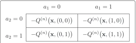
We formulate the optimization problem in thenth itera-tion of DP by a 2-player 2-strategy game, which is called one-stage game in Fig. 3. Assume that actiona1is taken by player 1, anda2is taken by player 2. Obviously, it is a pure coordination game where the utility−Q(n)(x,(a1,a2))is the same to player 1 and 2.
We prove, in Appendix D, that Fig. 3 is a supermod-ular game with utility function−Q(n)(x,(a
1,a2))strictly supermodular ina=(a1,a2)for allxandV(n−1)(x)that isL-convex inb=(b1,b2). It is proved in [30] that there exists at least one equilibrium(a∗1,a∗2)in the form of pure strategy in a supermodular game. Then, we have the fol-lowing theorem for the monotonicity of the optimal action a∗i inb=(b1,b2).
Theorem 4.13.If
(a) ξo ≥2λ+η+τ,
(b) one-stage game (in Fig. 3) has two pure strategy equilibria(0, 0)and(1, 1)for allx=(b1,b2,g1,g2) such thatbi<Li+1for alli∈ {1, 2},
then C(x,a) and Q(n)(x,a) are L-convex in (b,a) =
(b1,b2,a1,a2), the optimal value function V∗(x) is L
-convex inb=(b1,b2)and the optimal actiona∗=(a∗1,a∗2)
is nondecreasing inb=(b1,b2).
Proof. The proof is in Appendix E.
Here is a corollary of Theorem 4.13.
Corollary 4.14.If
(a) ξo≥2λ+η+τ, (b) p1=p2=0.5, (c) β ≤ 2(ττ+−ηλ),
then Theorem 4.13 holds.
Proof. The proof is in Appendix F.
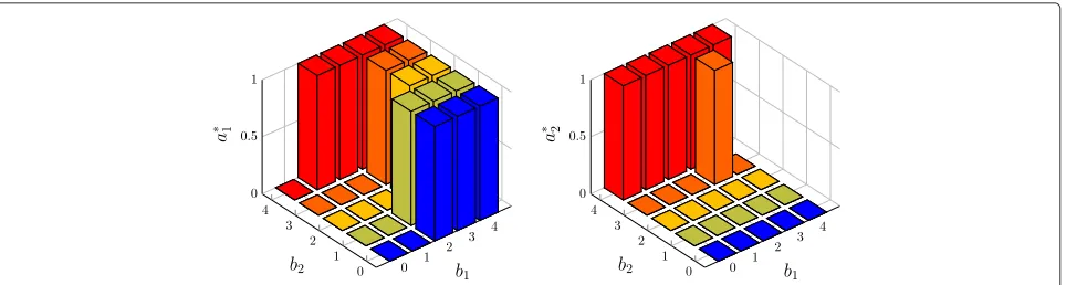
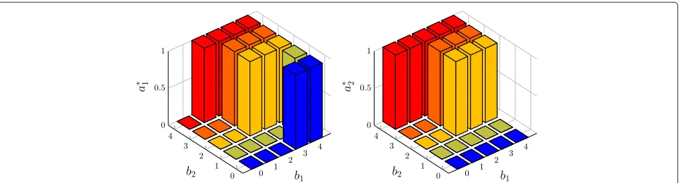
We show examples of Theorems 4.12 and 4.13 in Figs. 4, 5, 6 and 7. The results are collected by value iteration, a DP algorithm, applied on an NC-TWRC system with Bernoulli packet arrivals, 5 queue states, and 8 channel states, i.e.,fi(t) ∼ Bernoulli(pi), Li = 3 andKi = 8 for alltandi ∈ {1, 2}. In Fig. 4, we choose the values of unit costs to make Theorem 4.12 hold. As shown in the figure, the optimal actiona∗1anda∗2are monotonic inb1andb2, respectively, i.e., a∗i is nondecreasing in the queue state that is being controlled byai. In Fig. 5, we change the value of unit costξoto breach the condition in Theorem 4.12 so that the monotonicity ofa∗i inbiis not guaranteed. In this case,a∗1that is not monotonic inb1.
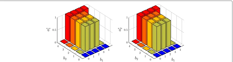
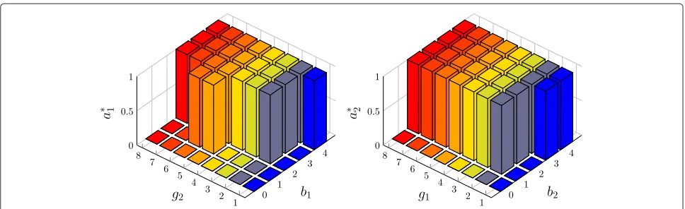
In Fig. 6, we choose the equiprobable packet arrival rates p1 = p2 = 0.5 and the unit costs according to Corol-lary 4.14 to make Theorem 4.13 hold. As shown in the
figure, the optimal actiona∗1anda∗2are both nondecreas-ing in (b1,b2). As compared to Fig. 4, in this case,a∗i is also monotonic inb−i, the queue state that is affected by the message flow and transmission control in the oppo-site direction, i.e., the queue state that is not controlled by ai. In Fig. 7, we switch unit cost η from 1 to 2 so that Theorem 4.13 no longer holds. In this case, neither a∗1nor a∗2is monotonic in(b1,b2). But, the condition in Theorem 4.12 is satisfied. Therefore, a∗1 anda∗2 are still nondecreasing inb1andb2, respectively.
4.3 Monotonic policies in channel states
The related research work in the existing literature con-siders the structure of the optimal policy in queue state only, e.g., [19, 21, 24]. This section breaks this limitation in that we extend the investigation of the monotonicity to the channel states. The main results are summarized as follows.
Theorem 4.15. If
(a) ξo≥2λ+η+τ, (b) Pe(gi)≥Pe(gi+1), (c) Pgig
iis first order stochastic nondecreasing ingi,
(d) β≤ Pe(gi)−Pe(gi+1) giPgigi(Pe(gi)−Pe(gi+1))
.
then C(x,a) and Q(n)(x,a) is submodular in(bi,g−i,ai), V∗(x)is submodular in(bi,g−i),and the optimal action a∗i is nondecreasing in(bi,g−i).
Proof. The proof is in Appendix G.
In Theorem 4.15, condition (b) is straightforwardly sat-isfied because of the definition ofPein (8) and assumption A4. Conditions (c) and (d) depend on the fading statistics and the FSMC modeling method. In fact, condition (c) is not hard to satisfy.
Fig. 4The optimal actiona∗1(left) anda∗2(right) vs. queue statesb1andb2wheng1=1 andg2=2.p1=0.1,p2=0.2,λ=0.05,τ=1,η=2,
Fig. 5The optimal actiona∗1(left) anda∗2(right) vs. queue statesb1andb2wheng1=1 andg2=2.p1=0.1,p2=0.2,λ=0.05,τ=1,η=2,
ξo=1, andβ=0.97. In this case,ξo<2λ+η+τ. Theorem 4.12 no longer holds. As can be seen,a∗1is not monotonic inb1
Corollary 4.16.If the FSMC of channel i adopts
equiprobable partitioning (of the full range of SNR), and channel i experiences slow and flat Rayleigh fading, then condition (c) in Theorem 4.15 are satisfied.
Proof.The proof is in Appendix H.
We show examples of Theorem 4.15 in Figs. 8 and 9. In Fig. 8, we use the same system parameters as in Fig. 4 except that the discount factorβ is switched from 0.97 to 0.95 in order to satisfy the inequality in condi-tion (d) of Theorem 4.15. The results are obtained from an NC-TWRC system where the channels experience slow and flat Rayleigh fading with average SNR γ1 = γ2 = 0dB. Both FSMCs are 8-state and adopt equiprob-able partition method. In this case, all the conditions in Theorem 4.15 are satisfied according to Corollary 4.16. Therefore,a∗1is nondecreasing in(b1,g2), anda∗2is non-decreasing in(b2,g1). In Fig. 9, we switch γ2 from 0dB to 3dB to breach condition (d) in Theorem 4.15. In this case,a∗1is not monotonic ing2. But, since Theorem 4.12 still holds, a∗1 and a∗2 are monotonic in b1 and b2, respectively.
Note, that the related previous studies usually placed constraints on the environments or the DP functions in order to prove the structure in the optimal policy. For example, in [19] the submodularity of the state transi-tion probability was proved by assuming uniformly dis-tributed traffic rates, and in [31], the strict submodularity ofQ(n)in DP iterations was assumed to be preserved by a weight factor in the immediate cost function (however, the exact value of this factor was not given). In contrast, the basic result in this paper, Theorem 4.12, is essen-tially given in terms of unit costs and discount factor, the parameters in the MDP model. The practical meaning of Theorem 4.12 can be interpreted in two ways. If the unit costs and discount factor are adjustable, we can tune them to get a structured optimal policy. If they are given, we can check the sufficient conditions for the existence of a monotonic optimal policy after the MDP modeling. In addition, we also derive the results, Theorems 4.13 and 4.15 by considering the uniform traffic rates, stochas-tic dominance of channel transition probabilities and channel modeling, and modulation scheme in this paper. They are also applicable if the associated conditions are satisfied.
Fig. 6The optimal actiona∗1(left) anda∗2(right) vs. queue statesb1andb2wheng1=1 andg2=5.p1=p2=0.5,λ=0.05,τ=1,η=1,ξo=4,
Fig. 7The optimal actiona∗1(left) anda∗2(right) vs. queue statesb1andb2wheng1=1 andg2=5.p1=p2=0.5,λ=0.05,τ=1,η=2,ξo=4,
andβ=0.97. In this case,ξo≥2λ+η+τbutβ >2(ττ+−ηλ). Theorem 4.12 holds, while Theorem 4.13 does not. As can be seen,a∗1anda∗2are monotonic inb1andb2, respectively, buta∗1is not monotonic inb2
5 Low complexity algorithms
This section considers the question of how to exploit the results in Section 4 to simplify the optimization process of problem (11). For this purpose, we present MPI and DSPSA algorithms for the MDP model in Section 3.
5.1 Monotonic policy iteration The idea of MPI is to modify (12) as
V(n)(x)= min a∈A(x)Q
(n)(x,a),∀x (19)
where A(x) ⊆ A is a selection of actions in A = {(0, 1)}2 = {(0, 0),(0, 1),(1, 0),(1, 1)}. Let θ(n)(x) = arg mina∈A(x)Q(n)(x,a). Note,θ(n)(x)can be obtained at the same time when V(n)(x) is calculated. We express
θ(n)(x)as
θ(n)(x)=θ(n)(b
1,b2,g1,g2)
=θ(n)
1 (b1,b2,g1,g2),θ (n)
2 (b1,b2,g1,g2)
. (20)
Assume that Theorem 4.13 holds. We can define the action selection set A(x) as follows. Due to the L -convexity ofQ(n)in(b
i,ai),θi(n) is always nondecreasing inbi. Therefore, we can defineA(x)as
A(x)=
a1∈ {0, 1}:a1≥θ1(n)([b1−1]+, [b2−1]+,g1,g2)
×a2∈{0, 1}:a2≥θ2(n)([b1−1]+, [b2−1]+,g1,g2)
whenb1=0 andb2=0 andA(x)=Awhenb1=b2= 0. For example, consider the case wheng1=1 andg2=1 at some iterationn. We need to determine the value of θ(n)(x)for allx=(b
1,b2,g1,g2)such thatg1=1 andg2= 1. We start with the lowest values ofb1andb2. For state
x=(0, 0, 1, 1), we haveA(x) = A= {0, 1}2. In this case, the minimization problem mina∈A(x)Q(n)(x,a) is equiv-alent to mina∈AQ(n)(x,a), i.e., we need to obtain four values ofQ(n)(x,a) ata = (0, 0),(0, 1),(1, 0), and (1, 1) to determine the minimum. If we getθ(n)(x) = (0, 1)for
x= (0, 0, 1, 1), thenA(x) = {0, 1} × {1} = {(0, 1),(1, 1)} forx=(0, 1, 1, 1),(1, 0, 1, 1)and(1, 1, 1, 1). It means that
Fig. 8The optimal actiona∗1vs. queue stateb1and channel stateg2whenb2=3 andg1=3 (left), anda∗2vs.b2andg1whenb1=2 andg2=1 (right).p1=0.1,p2=0.2,λ=0.05,τ=1,η=2,ξo=4 andβ=0.95. Two channels are both Rayleigh fading withγ1=γ2=0dB and are both modeled by 8-state equiprobable FSMCs. In this case,β≤ Pe(gi)−Pe(gi+1)
giPgigi(Pe(g
i)−Pe(gi+1))
, and according to Corollary 4.16, Theorem 4.15 holds. Therefore,
Fig. 9The optimal actiona∗1vs. queue stateb1and channel stateg2whenb2=3 andg1=3 (left), anda∗2vs.b2andg1whenb1=2 andg2=1 (right).p1=0.1,p2=0.2,λ=0.05,τ=1,η=2,ξo=4 andβ=0.95. Two channels are both Rayleigh fading and are both modeled by 8-state
equiprobable FSMCs. But,γ1=0dB andγ2=3dB. In this case,β≤ Pe(gi)−Pe(gi+1) giPgigi(Pe(g
i)−Pe(gi+1))does not hold for allgi. We can see thata ∗
1is not monotonic ing2
only two calculations ofQ(n)(x,a)are required when we want to determine the value of mina∈A(x)Q(n)(x,a) for these three states. In addition, if we find thatθ(n)(x) = (1, 1)forx= (1, 1, 1, 1), then, for allxsuch thatb1 > 1,
b2 > 1,g1 = 1 andg2 = 1,A(x) = {(1, 1)}and we can directly assign θ(n)(x) = (1, 1) without doing the min-imization mina∈A(x)Q(n)(x,a). We can find the optimal policy by repeating this process for all values ofg1andg2 in each iteration. From this example, it can be seen that (19) should be conducted in the increasing order of b1 andb2so that the cardinality of setA(x)is progressively reducing.
5.2 Discrete simultaneous perturbation stochastic approximation
Assume Theorem 4.12 holds.8Due to the monotonicity of the optimal policy in queue states, the optimization prob-lem (11) can be converted to a minimization probprob-lem over a set of queue thresholds.
Fori∈ {1, 2}, we defineφi(b−i,g1,g2)∈Bias
φi(b−i,g1,g2)=min{bi:θi(x)=1},∀b−i,g1,g2. (21)
Here, φi(b−i,g1,g2) is the threshold to queue i when the other user’s queue state isb−iand channel states are g1 and g2. Let φi be constructed by stacking φi for all
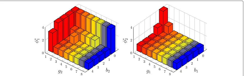
(b−i,g1,g2)∈B−i×G1×G2. The queue threshold vector is defined asφ=(φ1,φ2). In Fig. 10, we show the optimal queue threshold vectorφ∗=(φ∗1,φ∗2)where
φi∗(b−i,g1,g2)=min{bi:θi∗(x)=1},∀b−i,g1,g2 (22)
andθ∗is the optimal policy obtained in Fig. 4. Each queue threshold vectorφ= (φ1,φ2)determines a deterministic policyθφ(x)=(θ1φ1(x),θ2φ2(x))by
θiφi(x)=I{bi≥φi(b−i,g1,g2)}=
1 bi≥φi(b−i,g1,g2) 0 bi< φi(b−i,g1,g2) .
(23)
Since θi∗ is nondecreasing in bi for all i ∈ {1, 2} if Theorem 4.12 holds andθ∗determinesφ∗via (22), finding the optimal policyθ∗is equivalent to finding the optimal queue threshold vectorφ∗. We can convert problem (11) to
min
φ J(φ), (24)
where
J(φ)=
x(0)∈X E
∞
t=0
βtC(x(t),θ
φ(x(t)))|x(0)
. (25)
The advantage of formulating problem (24) is that the solutions can be approximated by the DSPSA algorithm [32] presented in Algorithm 1. The parameters/functions in this algorithm are explained as follows
• ˆJ(φ)is an estimation ofJ atφthat is obtained by simulation. The method is to simulate the state sequence{x(t)}governed by the transition probability
Pr x(t+1)|x(t)=Pθφ(x(
t))
x(t)x(t+1)for allx(0)∈X.ˆJ(φ)is obtained as
ˆ
J(φ)=
x(0)∈X T
t=0
βtCx(t),θ
φ(x(t))
. (26)
Each simulation stops if the increments over several successive decision epochs blow a small threshold (10−5), i.e., the simulation length is finite.
• The step size parametersA, B, andαare crucial for the convergence performance of DSA algorithms. In this paper, we set asA=0.3,B=100, and
Fig. 10The optimal thresholdφ1∗vs.b2andg2wheng1=2 (left), andφ2∗vs.b1andg1wheng2=1 (right). The system parameters are the same as in Fig. 4 so that Theorem 4.12 holds
where the computation budgetN, the total number of iterations, is fixed:B=0.095N,α=0.602andA is chosen so thatA/(B+1)αdφ˜(0) =0.1.
The DSPSA algorithm is a in fact a line search algorithm. It starts with any initial guessφ(0), sayφ(0)=0, and itera-tively updates the guess by the estimated descent direction −a(n)d(φ(n)). The gradient d(φ(n)) in each iteration is obtained based on two values ofˆJ,ˆJ φ(n) +1+2and ˆ
J φ(n) + 1−2.9According to a study in [34], the esti-mation sequence {φ(n)} slowly converges to the optimal queue threshold vectorφ∗.
Algorithm 1:DSPSA [32]
input : initial guessφ(0), total number of iterationsN, step
size parametersA,Bandα
output: [φ(N)], the closest integer point toφ(N)by Euclidean distance.
begin
forn=0to Ndo
a(n)=(B+n+A1)α;
Generate=(1,. . .,D)with each tuple
d∈ {−1, 1}being independent Bernoulli random
variable with probability 0.5. Obtaind(φ(n))with theith entry being
di(φ(n))=
ˆ J
φ(n) +1+
2
−ˆJ
φ(n) +1−
2
−1
i ,
(27)
wherexis the largest integer less thanx;
φ(n+1)=φ(n)−a(n)d(φ(n));
endfor end
5.3 Complexity
MPI is in fact a modified DP algorithm that exploitsL -convexity or submodularity of Q(n). It converges at the same rate as DP. But, sinceA(x)⊆Aand|A(x)|, the car-dinality ofA(x), is progressively decreasing inb1andb2, the complexity in each iteration in MPI is lower than that in DP. Letρbe the average size ofA(x)over all statesx. The complexity in one iteration of MPI isO(|X|2ρ), where
ρ ≤ |A|. The exact value ofρ varies with different sys-tems. To show the examples of the actual complexity of MPI, we do the following experiment. We use the same system settings as in Fig. 6 and set the number of chan-nel states of both chanchan-nels toK, i.e.,K1 = K2 = K. We vary K from 2 to 10. For each value ofK, we run both DP and MPI and obtain the complexity as the number of calculations ofQ(n) averaged over iterations. The results are shown in Fig. 11. It can be seen that the complexity of MPI is always less than that of DP, and MPI alleviates the
drastically growing complexity in DP when the size of the channel state space grows large.
Consider the complexity of the DSPSA algorithm. Letζ be the complexity of obtaining the value ofˆJby simulation. Since we only need two values ofˆJto calculate the gradi-entd, the complexity in each iteration of DSPSA isO(ζ). But, the convergence rate depends on the parameters of the DSPSA algorithm [35], e.g., the step size parameters, and may vary with different MDP systems, i.e., DSPSA may converge slower than DP or MPI. However, we have two advantages of implementing DSPSA algorithm over DP or MPI. One is that DSPSA is a simulation-based algo-rithm, the runs of which do not require the full knowledge of the MDP model. Based on (26), to obtainJˆ, we only require the knowledge of the state space X and a sim-ulation model that can generate a state sequence {x(t)}
based on a given queue threshold vectorφand the statis-tics of packet arrival and channel variation processes. If the packet arrival probabilities and/or channel statistics change suddenly, the optimal policy will change accord-ingly, and DSPSA algorithm can adapt slowly to the new optimal policy.
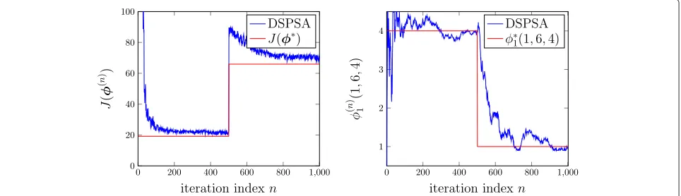
The results in Fig. 12 are based on an experiment of DSPSA in an environment where the system parame-ters change with time. The relay is assumed to serve the first pair of users with packet arrival probabilities being p1 = 0.1 and p2 = 0.2 in the first 500 iterations and serve another pair of users withp1 = 0.8 andp2 = 0.2 in the second 500 iterations. It can be seen that DSPSA is able to adaptively track the optimum and optimizer of problem (24). In contrast, to run DP or MPI, we require the full knowledge of the MDP model. If the statistics of packet arrival and channel variation processes change, we need to determine the new MDP model by calculat-ing all values of the state transition probabilityPxxa before
running DP or MPI. Alternatively speaking, MPI and DP are model-based algorithms while DSPSA is a model-free algorithm [36].
The other advantage of DSPSA is that it allows the scheduler to learn the optimal policy online. For exam-ple, assume that we start with any arbitrary threshold vector φ(0). We first let the scheduler adopt the pol-icy that is determined by the queue threshold vector φ(0) + 1+
2 (via (21)) for a while and obtain the value ofˆJ φ(0) + 1+2based on the actual immediate costs incurred. Then, we let the scheduler adopt the policy that is determined byφ(0) + 1−2for a while and obtain the value ofˆJ φ(0) +1−2. By doing so, the gradientdcan be calculated, and we update φ(0) and get a new queue vectorφ(1). By repeating this process, the scheduler can slowly update the estimationφ(n) towardsφ∗and hence find the the optimal policyθ∗.
It should be noted that low complexity algorithms for searching or approximating the optimal policy θ∗ are not restricted to MPI and DSPSA. With the results on monotonicity derived in Section 4, one can propose other algorithms, e.g., the random search method [37], the sim-ulated annealing method [38], the complexity of which could be even lower than MPI and DSPSA. For example, the random search method [37] can be applied to find the solution of the multivariate minimization problem (24). In this method, the descent direction is found by random sampling in each iteration. The complexity incurred by random sampling could be lower than that incurred by simulation (as in DSPSA). But, we still need to compare the convergence rates of the random search and DSPSA algorithms. In summary, the MPI and DSPSA are two examples of low complexity algorithms that are based on the monotonicity of the optimal policy. To propose more low complexity algorithms and compare the convergence
Fig. 12Convergence performance of DSPSA:J(φ(n)), the value of the objective function at thenth iteration of DSPSA (left);φ1(n)(1, 6, 4), the estimations of the optimal threshold to queue 1 whenb2=1,g1=6 andg2=4 (right). The channels are both Rayleigh fading with
γ1=γ2=0dB and modeled by 8-state FSMCs. The system parameters are set asp1=0.1,p2=0.2,λ=0.05,τ=1,η=2,ξo=4 andβ=0.97
performance are out of the scope of this paper and could be one of the future directions of research.
5.4 Simulation results
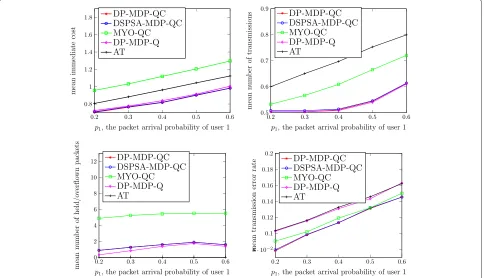
We run simulations in an NC-TWRC with Rayleigh fad-ing channels. Let DP-MDP-QC be the optimal policy searched by DP based on the MDP model in Section 3. We compare the performance of DP-MDP-QC to the following four policies:
• DSPSA-MDP-QC: This policy is searched by DSPSA
based on the MDP model in Section 3 with the total number of iterations beingN=1000. As explained in Section 5.2, the estimation sequence produced by the DSPSA algorithm should be slowly converging to the optimal policy. Therefore, DSPSA-MDP-QC should be close to DP-MDP-QC (in Euclidian distance) and the performance of DSPSA-MDP-QC should be similar to that of DP-MDP-QC.
• MYO-QC: This policy is obtained by
θMYO-QC(x)=arg minaC(x,a), whereC(x,a)is the immediate cost function as defined in (9). Recall that policy DP-MDP-QC searched by DP isθ∗(x)= θN(x)=arg min
aC(x,a)+βxPxxa V(N−1)(x), whereN is the iteration index when DP converges. MYO-QC is the policy that neglects the aftermath βxPaxxV(N−1)(x)that is incurred by the action taken at the current decision epoch. Alternatively speaking, MYO-QC is myopic while DP-MDP-QC is far-sighted.10In a stochastic environment, myopic policies usually incur a higher expected long-term cost than far-sighed ones.
• AT: This policy is denoted as
θAT(x)=(θAT1(x),θAT2(x))whereθATi(x)=1if bi=0, i.e., always transmit whenever queuei is not empty. This policy minimizes the costs incurred by the packet delay and queue overflow. But, the performance of this policy should not be as good as DP-MDP-QC if the purpose is to minimize the long-term cost incurred by not only the packet delay and queue overflow but also the transmission power consumption and downlink transmission error rate.
• DP-MDP-Q: This policy is determined by DP based on an MDP model that is the same as the one in Section 3 except that the immediate cost function is defined asC(x,a)=Ch(b,a)+tr(a). This policy was proposed in [12], where the authors assume that the channels are lossless so that the packet error cost
2
i=1err(g−i,ai)=0always. However, the wireless channels are usually not ideal in practice. If we adopt policy DP-MDP-Q, it should incur a higher downlink transmission error rate than DP-MDP-QC.
We fixp2= 0.5 and varyp1from 0.2 to 0.6. The other system parameters are the same as in Fig. 4. A simulation lasting for 105decision epochs is run for each value ofp
1. Each packet contains 100 bits, i.e., the packet lengthLP = 100. We obtain the number of holding and overflowing packets and the number of transmissions averaged over decision epochs. The former indicates the mean packet delay and queue overflow costs, and the latter indicates the average transmission power consumption. The trans-mission error rate is calculated as the ratio of the number of erroneous bits received to the total number of bits sent. We also obtain the immediate cost averaged over decision epochs, which indicates the long-term cost (the minimand in (11)). The results are presented in Fig. 13. It can be seen that the average immediate cost of DSPSA-MDP-QC almost overlaps with that of DP-DSPSA-MDP-QC. It means that if we allow the total number of iterations in the DSPSA algorithm large enough, e.g., 1000 iterations, it is able to converge to a policy that is very close to DP-MDP-QC.
For policy MYO-QC, we can see that it always incurs a greater number of transmissions and holding and over-flow packets and a higher transmission error rate than DP-MDP-QC. The average immediate cost of this policy is at least 0.23 higher than those of DP-MDP-QC, which is the worst among all policies. Therefore, a far-sighted pol-icy outperforms a myopic one when we want to minimize the long-term cost in a stochastic system.
The number of holding and overflow packets incurred by policy AT is always zero. However, it results in the high-est number of transmissions and transmission error rate. The average immediate cost incurred by AT is at least 0.09 higher than DP-MDP-QC, which justifies our expec-tation; AT minimizes the packet delay and queue overflow costs but incurs higher transmission power consumption and downlink transmission error rate. Therefore, the long-term cost incurred by AT is not as low as that incurred by DP-MDP-QC. For policy DP-MDP-Q, the number of transmissions is almost the same as DP-MDP-QC, and the number of holding and overflow packets is even lower than DP-MDP-QC. However, since this policy assumes that the wireless channels are ideal (but they are in fact not), the transmission error rate is about 1.3 times higher than DP-MDP-QC (almost as high as AT). Therefore, the average immediate cost is still higher than DP-MDP-QC. In summary, in a stochastic environment where the long-term loss can be incurred by multiple causes, the policy that considers all such causes simultaneously outperforms those that only consider some and neglects others.
6 Conclusion
Fig. 13Simulation results: the mean immediate costC(x,a)(top left); the mean number of transmissionsI{a1=1 ora2=1}(top right); the mean number
of holding packets min{[yi]+,Li}(bottom left); the mean number of lost packets due to queue overflowI{[yi]+=Li+1}, and the mean transmission error rate (bottom right). These are the values averaged over 105decision epochs. The channels are both Rayleigh fading withγ
1=γ2=0dB and modeled by 8-state FSMCs. The system parameters are set asp2=0.5,λ=0.05,τ=1,η=2,ξo=4 andβ=0.97.p1is varying from 0.2 to 0.6
monotonic optimal transmission policy that minimized packet delay, queue overflow, transmission power, and the downlink transmission error rate in the long run. We proved that the optimal policy is nondecreasing in queue and/or channel states by investigating how certain properties (submodularity,L-convexity and multimodu-larity) varied with the system parameters. Based on these properties of DP, we presented two low-complexity algo-rithms, MPI and DSPSA.
As a part of the conclusion, we point out two direc-tions for the research work in the future. The structured results derived in Section 4 can be used to design model-free learning algorithms, e.g., monotonic Q-learning. Since queue-assisted transmission control is also used in cross-layer variable-rate adaptive modulation problems, it would be of interest if we can use submodularity,L -convexity, and multimodularity to establish the sufficient conditions for the existence of monotonic optimal trans-mission policies in these systems.
Endnotes
1The complexity of the algorithm grows drastically
with the cardinality of the system variables [16]. 2The definition of Pareto optimality is given in
Appendix A. In Section 3.5, we will explain the Pareto optimality of the optimal policy of MDP.
3In this paper, we use=10−5.
4See the definition of Pareto optimality and description
of scalarization technique in Appendix A. The Pareto optimality ofθ∗has also been discussed in [31].
5f:Zn→R
−is (strictly) supermodular if−f is (strictly) submodular.
6The interpretation ofξ
o≥2λ+η+τis that the cost of overflowing a packet is greater than or equal to the sum of the cost of holding two packets, the cost when transmission error rate is increased byηand the cost of missing a coding opportunity.
7In [21], integer convexity was used to denote the one
dimensional discrete convexity as explained in Lemma B.1(b).
8According to the conditions in Theorems 4.12, 4.13
and 4.15, Theorem 4.12 is straightforwardly satisfied if either Theorem 4.13 or Theorem 4.15 holds. Therefore, if DSPSA can be applied when Theorem 4.12 holds, it can be also applied when Theorem 4.13 and 4.15 hold.
9The gradientdin (27) is defined based on the discrete
mid-point convexity [32].
10More comparisons of far-sighted and myopic policies
in NC-TWRC are presented in [13].
allx ∈ Z. Moreover, by Definition 4.4 and 4.5,his both L-convex and multimodular.
12A functionf:Z2→R
+is multimodular if and only if it is (1) supermodualr:ijf(x)≥0 and (2) superconvex:
if(x + ei) ≥ if(x + ej) for alli,j ∈ {1, 2}, where
if(x) = f(x) − f(x − ei)andei∈Z2is a 2-tuple with all zero entries except theith entry being one.
Appendix A
In multi-objective optimization [39], there are N opti-mization metrics. Each of then can be quantified by a loss functionfn:RM→R. The problem can be expressed as
min
x∈RM(f1(x),f2(x),. . .,fN(x)), (28)
wherexis the decision vector. We sayxPareto dominates
x if fn(x) ≤ fn(x) for all n ∈ {1,. . .,N}. We call x∗ a Pareto optimal decision vector if nox∈RMPareto dom-inatesx∗. In a multi-objective optimization problem, we always want to seek a Pareto optimal solution. One way to solve this problem is called scalarization technique. The idea is to convert (28) to a single-objective problem
min
x∈RMw1f1(x)+w2f2(x)+. . .+wNfN(x)), (29)
wherewn>0 is the weight. It is shown that the solution of problem (29) is a Pareto optimal solution of problem (28) in [39]. Note, based on the definition of Pareto optimality, a Pareto optimal solution is not an optimal solution if we purely consider only one optimization metric.
Appendix B
Lemma B.1.submodularity, L-convexity and
multi-modularity has the following properties:
(a) Iffi: Zn→R+is
submodular/L-convex/multimodular inx∈Znand αi≥0for all i, thenmi=1αifi(x)is
submodular/L-convex/multimodular inx. (b) Ifh:Z→R+is convex11, thenf(x)=h(x [26, 28, 29]. We show proof of (c). Consider function f first. Sinceψ(x,ζ)= f(x−ζ1) = h(x1−x2), according to Definition 4.4, it suffices to show the submodularity of hin(x1,x2). But, because of the convexity ofh,
Cis nondecreasing iny1because h1is nondecreasing in
y1. By assuming thatV(n−1) is nondecreasing inb1, we have Q˜(n) nondecreasing in y1 since min{[yi]+,Li} +fi is nondecreasing inyi. Next, consider the multimodular-ity by using Proposition 112in [40]. The supermodulariry and superconvexity ofC˜ in(y1,a1)can be proved by the convexity ofh1. So,C˜ is multimodular in(y1,a1). Assume the monotonicity andL-convexity ofV(n−1) inb1.Q˜ is supermodular and superconvex in(y1,a1)because
Appendix D definition in [30], the game is supermodular.
Appendix E actiona∗is nondecreasing inb.
Appendix F
We just need to show that condition (b) in Theorem 4.13 is satisfied. Letbi−a1<Li+1 for alli∈ {1, 2}. It suffices
The second last inequality in (35) is obtained by using a similar approach as in (32), and the last one is due to the conditionβ ≤ Pe(gi)−Pe(gi+1)
In an equiprobable partitioned slow and flat Rayleigh fad-ing channel, the channel transitions can be worked out by level crossing rate (LCR) [15] and only happens between adjacent states, i.e.,gi∈ {gi−1,gi,gi+1}. Further,Pgg =
NC-TWRC: network-coded two-way relay channels; MDP: Markov decision process; DP: dynamic programming; MPI: monotonic policy iteration; DSPSA: discrete simultaneous perturbation stochastic approximation; NC: network coding; FSMC: finite-state Markov chain; QoS: quality of service; SPSA: simultaneous perturbation stochastic approximation.
Competing interests
The authors declare that they have no competing interests.
Received: 9 July 2015 Accepted: 20 October 2015
References
1. R Ahlswede, N Cai, S-YR Li, RW Yeung, Network information flow. IEEE Trans. Inf. Theory.46(4), 1204–1216 (2000). doi:10.1109/18.850663 2. Y Wu, Information exchange in wireless networks with network coding
and physical-layer broadcast. Technical Report MSR-TR-2004-78, Microsoft Research, Redmond WA (2004)
3. S Katti, H Rahul, W Hu, D Katabi, M Médard, J Crowcroft, Xors in the air: practical wireless network coding. SIGCOMM Comput. Commun. Rev. 36(4), 243–254 (2006)
![Fig. 2 NC-TWRC with random packet arrivals and fading channels [13]. The incoming packets are buffered by two finite length first-in-first-out (FIFO)queues](https://thumb-us.123doks.com/thumbv2/123dok_us/944576.1115172/2.595.57.291.87.136/random-packet-arrivals-fading-channels-incoming-packets-buffered.webp)