R E S E A R C H
Open Access
Non-data-aided ML SNR estimation for AWGN
channels with deterministic interference
Fangjiong Chen, Yabing Kang, Hua Yu
*and Fei Ji
Abstract
Communication channels not only suffer from ambient noise but also from deterministic interference. In this paper, we consider signal-to-noise ratio (SNR) estimation in the presence of constant deterministic interference. A maximum likelihood (ML) non-data-aided algorithm is proposed for SNR estimation. We first consider a real-valued model and then extend this to a complex-valued model. The proposed algorithm applies an iterative approach initialized with approximate closed form estimates so as to guarantee stability and convergence. Furthermore, the Cramer-Rao bound (CRB) is also derived as the theoretical limit of the jitter variance. Computer simulations based on
pulse-amplitude modulation (PAM) and quadrature amplitude modulation (QAM) sources show that the performance of the proposed algorithm is close to the CRB.
Keywords: SNR estimation; Maximum likelihood estimation; Non-data aided estimation; Cramer-Rao bound
1 Introduction
Besides ambient noise, the communication channels may suffer from deterministic interference. In terrestrial wire-less systems, the competing users sharing the same spec-trum resource, or simply the drift of the system’s baseline, may introduce some sort of deterministic interference [1,2]. When a direct conversion receiver is applied, the demodulator output is usually impaired by a direct cur-rent (DC) offset due to self-mixing [3], which might be considered as some sort of deterministic interference. More recently, based on an experimental underwater communication system, Wang et al. [4] observed that unknown users transmitting multiple sonar waveforms in the same environment may lead to significant perfor-mance degradation. In [4], the deterministic interference is modelled as known waveform with unknown param-eters. Interference reconstruction and cancelation was applied to improve the system performance.
The signal-to-noise ratio (SNR), defined as the ratio of the signal power to the noise power, is frequently used as the system performance measure [5-8]. In cases where interference is present, the interference can be estimated and removed from the estimated signal [2,3]. In [1,6,7], the signal-to-interference-plus-noise ratio (SINR), instead of
*Correspondence: [email protected]
School of Electronic and Information Engineering, South China University of Technology, Guangzhou 510640, China
SNR, is applied as the system measure. In [1], a non-data-aided (NDA) algorithm, based on fourth-order statistics, was proposed for SINR estimation, where the interference was modeled as a constant. In [6] and [7], SINR estimation in cellular systems is investigated, where the interference stems from competing users in other cells.
In [6,7], the interference was modelled as zero-mean random variable. The algorithms indeed cannot deal with deterministic interference. The fourth-order statistics-based algorithm in [1] requires a large quantity of samples (more than 1,000). It may not be effective to assume that the interference is constant during thousands of symbols. The maximum likelihood (ML) algorithm in [2] needs only tens of samples. However, the algorithm assumes no attenuation of the source signal and hence is not applica-ble to SNR estimation.
Our goal in this paper is to develop a NDA SNR esti-mation algorithm which provides satisfactory estimates with a small size of samples (e.g., tens of samples). We assume a slowly time-varying channel such that over the observation interval, the channel gain and the interference can be assumed to be constant. In natural, therefore, this is an additive noise channel model with attenuation fac-tor and deterministic interference during the observation interval.
In this paper, an iterative maximum likelihood (ML) algorithm is proposed for SNR estimation. A sim-ple moment-based estimator is applied to initialize the ML algorithm. Simulation results show that the pro-posed algorithm converges within 10 iterations. We also derive the theoretical performance bound, i.e., the Cramer-Rao bound (CRB) as the performance bench-mark. Computer simulations based on pulse-amplitude modulation (PAM) and quadrature amplitude modula-tion (QAM) sources show that the performance of the proposed algorithm with tens of samples is close to the CRB.
2 Development of the iterative ML algorithm
2.1 Real-valued system with PAM signaling
We first consider a real-valued system with PAM signal-ing. The received signal is given by
xn=Asn+I+vn, (1)
wheresnis the source signal andvnis the ambient noise. We assume that vn is zero-mean white Gaussian noise with variance σ2. A stands for the channel gain/atten-uation, andIis the deterministic interference. We assume that sn is generated randomly by aM-ary PAM source with equiprobable constellation points at±(2m−1),m= 1, 2,· · ·,M/2, withM = 2p andp ∈ N. Therefore, the average power of aM-ary PAM signal is given byEM
PAM = (M2−1)/3. As a result, the SNR of the received signal is
defined as
γ = A
2EM PAM
σ2 . (2)
We note that in the open literature [1], the SINR, defined asγ = A2EPAMM
I2+σ2 has also been applied as the per-formance measure. On top of that, cancellation of the DC offset is discussed in [3] and [9], where the SNR is used as the major figure of merit (it was argued that the DC offset has a less significant impact on the system perfor-mance than noise [3]). In the current paper, the constant deterministic interference (i.e. the DC-offset) was esti-mated and suppressed from the received signal, and then the SNR is applied as the performance measure. Our the-oretical analysis further shows that varying the value of deterministic interference has no effect on the accuracy of parameter estimation (i.e. the estimation of A, I and
σ2; see also Section 3). Hence, we argue that the SNR is a more proper performance measure in the presence of deterministic interference.
We shall separately estimate A,I,σ2 and then use these estimates to calculateγ. Without loss of generality, Ais assumed to be a positive number in this paper. The PDF ofxnis given by
f(xn)= 1 M√2π σ2
M/2
m=1
exp
−(xn−I−A(2m−1))2 2σ2
+ exp
−(xn−I+A(2m−1))2 2σ2
= 2
M√2π σ2exp
−(xn−I)2 2σ2
M/2
m=1
exp
−A2(2m−1)2 2σ2
cosh
A(xn−I)(2m−1)
σ2
.
(3)
Assume there are N available samples, denoted as x = [x1,x2,· · ·,xN]. Since the transmitted symbols are assumed to be independent and identically distributed (i.i.d.) and the additive noise is white, then the corre-sponding received samples are independent and their joint probability density function (PDF) is simply the product of the PDF of each sample. Consequently, the log-likelihood function ofxis given by
L(x)=ln N
n=1
f(xn)=Nln
2 M√2π σ2
− N
n=1
(xn−I)2 2σ2
+ N
n=1
ln
⎛
⎝M
/2
m=1
hcm,n
⎞
⎠, (4)
wherehcm,nis given as
hcm,n=exp
−A2(2m−1)2 2σ2
cosh
A(xn−I)(2m−1)
σ2
,
(5)
By forcing the derivatives ∂L∂(Ax), ∂L∂(Ix), ∂∂σL(x2) to zero, we obtain the subsequent relationships:
A=
N
n=1(xn−I)Hns
N
n=1Hnc
, (6)
I = 1 N
N
n=1
xn−AHns
, (7)
σ2 = 1
N N
n=1
(xn−I)2+A2Hnc−2A(xn−I)Hns
,(8)
where
Hnc = M/2
m=1
(2m−1)2hcm,n M/2
m=1hcm,n
, (9)
Hns = M/2
m=1
(2m−1)hsm,n M/2
m=1hcm,n
, (10)
hsm,n=exp
−A2(2m−1)2 2σ2
sinh
A(x
n−I)(2m−1)
σ2
. (11)
which has to be initialized properly. For this purpose, we consider the initialization based on the moments of the received signal.
By directly calculating the first-order sample raw moment of the received signal, we obtain the following initialization ofI:
ˆ I0=
1 N
N
n=1
xn. (12)
The second- and fourth-order central moments of the signal population are respectively given as,
μ2=Es,v
(xn−I)2
=Es,v
(Asn+vn)2
=A2Es2n+Ev2n=A2ν2+σ2, (13) μ4=Es,v
(xn−I)4
=Es,v
(Asn+vn)4
=A4ν4+6A2ν2σ2+3σ4, (14)
whereν2=E
s2
n
=EM
PAMandν4=E
s4
n
are the second-and fourth-order raw moments of theM-ary PAM signal {sn}, respectively. And
ν4= 2
M M/2
m=1
(2m−1)4= 1
15
3M2−7 M2−1.
(15)
According to (13) and (14), one has an equation forAas
3μ22−μ4=A43ν22−ν4. (16)
Equating the population moments with the sample moments, one moment-based estimator for A can be derived as
ˆ A0=
3μˆ22− ˆμ4
3ν22−ν4
1/4
, (17)
whereμˆ2andμˆ4are the second- and fourth-order sample
central moments of the received signal and are given by, respectively,
ˆ
μ2=
1 N
N
n=1
xn− ˆI0
2
, μˆ4=
1 N
N
n=1
xn− ˆI0
4
.
(18)
When ˆI0 and Aˆ0 are available, σ2 can be estimated
by exploiting the second-order central moment of the received signal, as follows:
ˆ
σ02= 1
N N
n=1
xn− ˆI0
2
− ˆA20EM
PAM. (19)
As a result, the moment-based estimator forγ can be expressed as
ˆ
γ0=
ˆ A0EPAMM
ˆ
σ02 . (20)
These moment-based estimators are only valid in the high SNR range. Unfortunately, they usually require a large quantity of samples to obtain accurate estimation, which is not realistic in practical time-varying systems. In order to obtain a more accurate estimation and speed up the convergence, we propose that the iterative method in (6) to (8) is initialized by the closed form estimates given by (12), (17) and (19). The procedure stops when a prede-fined maximum of iterations is achieved or when the error is lower than a specified value. The algorithm is outlined in Algorithm 1, whereK is a predefined maximal num-ber of iterations,εis a predefined small constant, and the iterative errorεkis defined as
εk =
ˆ
γk− ˆγk−1
ˆ
γk 2
, k=1, 2,· · ·. (21)
Algorithm 1Iterative ML SNR estimation algorithm for PAM signaling
Initialization:
Set k = 0, and calculate the initial estimation ofI,A andσ2, denoted as Iˆ0, Aˆ0andσˆ02based on (12), (17)
and (19), respectively; Iteration:
1: repeat
2: Calculate thek-th estimation of hcm,n and hsm,n by (5) and (11), respectively, withA,I, andσ2replaced byAˆk,ˆIkand σˆk2, respectively; denote the results as ˆ
hmc,n,kandhˆsm,n,k;
3: Calculate thek-th estimation of Hnc and Hns by (9)
and (10), respectively, withhcm,n and hsm,nreplaced byhˆcm,n,kandhˆsm,n,k, respectively; denote the results asHˆnc,kandHˆns,k;
4: k←k+1;
5: Calculate thek-th estimation ofA, Iandσ2by the equations (6), (7) and (8), respectively, withA,I,σ2, HnsandHncreplaced byAˆk−1,Iˆk−1,σˆk−2 1,Hˆns,k−1and
ˆ
Hnc,k−1, respectively; denote the results asAˆk,ˆIkand ˆ
σk2.
6: untilk=Korεk < ε. Output:
ˆ
Ak, Iˆk, σˆk2, and γˆk = ˆA2kEPAMM /σˆ 2
2.2 Complex-valued system with QAM signaling
Considering the complex-valued signal system, the signal model is revised as
rn=Gsn+I+wn =(A+jB)an+jbn
+(C+jD)+un+jvn
=(Aan−Bbn+C+un)+j(Ban+Abn+D+vn)
xn+jyn. (22)
We assumesn=an+jbnis aM-ary square QAM source, that is,sn∈S= {Siq=ai+jbq=(2i−1−2p)+j(2q−1− 2p),i,q = 1,· · ·, 2p}, whereM=22pfor any natural numberp,G= A+jBis the complex channel gain,I =C+jD andwn=un+jvnare respectively the complex interference and complex noise. The average power of the square QAM constellation power is given byEM
QAM=E
|Siq|2
=2(M−1)/3. The SNR of the received signal is defined as
γ = |G| 2EM
QAM 2σ2 =
A2+B2EM QAM
2σ2 . (23)
We shall separately estimate the unknown parameters of the vector{A,B,C,D,σ2} and then use these estimates to calculateγ. Without loss of generality,AandBare assumed to be positive numbers in this paper.
The joint PDF of the real and image parts ofrnis given by:
frn(xn,yn)=
1 2Mπ σ2
Siq∈S
exp
−
(xn−C)−(Aai−Bbq)
2+
(yn−D)−(Bai+Abq)
2
2σ2
= 1
2Mπ σ2exp
−(xn−C)2+(yn−D)2 2σ2
Siq∈S
exp
−|GSiq|2 2σ2
exp
(xn−C)(Aai−Bbq)+(yn−D)(Bai+Abq)
σ2
(24)
According to the symmetry of the square QAM constellation,frn(xn,yn)can be written as
frn(xn,yn)=
1 2Mπ σ2exp
−(xn−C)2+(yn−D)2 2σ2
Siq∈S
exp
−|GSiq|2 2σ2
exp
(A(xn−C)+B(yn−D))ai+(A(yn−D)−B(xn−C))bq
σ2
= 2
Mπ σ2exp
−(xn−C)2+(yn−D)2 2σ2
2p−1
i=1
exp
−(A2+B2)(2i−1)2 2σ2
cosh
(A(xn−C)+B(yn−D)) (2i−1)
σ2
2p−1
q=1
exp
−(A2+B2)(2q−1)2 2σ2
cosh
(A(yn−D)−B(xn−C)) (2q−1)
σ2
= 2
Mπ σ2exp
−(xn−C)2+(yn−D)2 2σ2
where
Assume there areNavailable received samples, denoted asr = [r1,r2,· · ·,rN]. As a result, the logarithmic likeli-(see Appendix) to zero, we obtain the following equations:
A= 1
Similar to the case of PAM signaling, we adopt the moment-based estimators as initialization and then apply iterative estimation based on (31) to (35) to refine the esti-mated results. At first, the moment estimate ofIis given as
The second- and fourth-order central moments of the signal’s real and imaginary parts are respectively given as,
μx2 =Es,w(xn−C)2=Es,u(Aan−Bbn+un)2 order raw moments of the real/imaginary part of theM -ary QAM signal{sn}, respectively. And
real/imaginary part of received signal, and are given by,
by exploiting the second-order central moment of the received signal, as follows:
ˆ
As a result, the moment-based estimator forγ can be expressed as metric such that they cannot be decoupled from these equations. Therefore, they are temporally assumed to be equal and then they are refined by the iteration. That is, the rough estimates ofAandBare given as
ˆ
A0= ˆB0=
| ˆG0|2/2. (55)
The iterative algorithm is similar to the case of PAM signaling and will not be shown here for saving space.
3 The Cramer-Rao bound
3.1 The real-valued system with PAM signaling
In this section, we derive the CRB for unbiased estima-tion of γ. Letθ = [θ1,θ2]= Fis the Fisher information matrix (FIM) defined as
F j =E
whereE{·}denotes the expectation w.r.t the random vari-ables{sn}and{vn}. After some algebra, we have (61). By using this kind of substitution, it is easily observed thatHncandHns do not includeIas well. For convenience,
white Gaussian noisevwith varianceσ2. It is not possible to obtain closed-form expressions for the above inte-grations. Numerical computation is applied to calculate
that, in theory, an increase of the interference level would not hurt the accuracy in estimatingA,σ2,γ.
3.2 The complex-valued system with QAM signaling Next, we consider the complex-valued system with QAM Signaling. Letθ =[θ1,θ2,θ3]=A,B,σ2andγ =g(θ)=
F is the Fisher information matrix, whose elements are defined as
where E{·}denotes the expectation w.r.t to the random variables{an},{bn},{un}, and{vn}.
With some calculation, we have (see Appendix)
∂L(r) In fact, since
xn−C = Aan−Bbn+un, (74) can be calculated by
F j =
is the joint PDF of the real and image parts of the complex additive white Gaussian noisew=u+jvwith varianceσ2. In the simula-tion, numerical computation is applied to calculateη j(s),
μ (s)and then the CRB.
4 Numerical results
Computer simulation results are presented to show the performance of the proposed algorithm. Unless otherwise specified, a sample size ofN = 80, 2×10⁴independent trials and an interference-to-noise ratio (INR) of 0 dB are applied in the simulation. To guarantee convergence,is set to a small value of 10−6andKis set to a large value of 100. To obtain a performance measure for a fair compari-son of different parameters, we use the normalized sample mean square error (NMSE) defined by
NMSE= 1
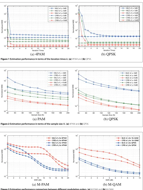
whereNtris the number of total independent trials andγˆi is the estimated value of the true SNRγ from theith trial. Figure 1 shows the convergence property of the pro-posed ML estimator (MLE). It can be observed that the algorithm has fast convergence speed since that it con-verges in several iterations, and the performance of the proposed MLE is close to the CRB and significantly out-performs the moment-based estimator (k=0).
Figure 2 shows the estimation performance under differ-ent sample sizes. It can be observed that the proposed ML estimator results in almost identical performance to the CRB. We therefore argue that tens of samples is enough to obtain efficient estimation. Although in this paper we assume time-invariant interference level and noise power, the proposed algorithm indeed is applicable to slow time-varying systems where the parameters can be assumed to be invariant within tens of samples. We also observe that an increased number of samples will be required to obtain an accurate SNR estimation, especially at low SNR.
0 2 4 6 8 10 12 14 16 18 20 10−1
100 101 102 103 104
Normalized MSE
Iteration Times
0 2 4 6 8 10 12 14 16 18 20 10−2
10−1 100 101 102 103
Normalized MSE
Iteration Times
MLE of γ= 0dB MLE of γ= 5dB MLE of γ=10dB CRB of γ= 0dB CRB of γ= 5dB CRB of γ=10dB
(a) 4PAM
(b) QPSK
MLE ofγ= 0dB MLE ofγ= 5dB MLE ofγ=10dB CRB ofγ= 0dB CRB ofγ= 5dB CRB ofγ=10dB
Figure 1Estimation performance in terms of the iteration timesk.(a)4PAM and(b)QPSK.
40 60 80 100 120 140 160 180 200 10−2
10−1 100 101 102
Sample Size (N)
Normalized MSE
MLE of γ = 0dB CRB of γ = 0dB MLE of γ = 5dB CRB of γ = 5dB MLE of γ =10dB CRB of γ =10dB
40 60 80 100 120 140 160 180 200 10−2
10−1 100
Normalized MSE
Sample Size (N)
MLE of γ= 0dB MLE of γ= 5dB MLE of γ=10dB CRB of γ= 0dB CRB of γ= 5dB CRB of γ=10dB
(a) PAM
(b) QPSK
Figure 2Estimation performance in terms of the sample sizeN.(a)4PAM and(b)QPSK.
0 2 4 6 8 10 12 14 16 18 20 10−2
10−1 100 101
SNR (dB)
Normalized MSE
0 1 2 3 4 5 6 7 8 9 10
10−2 10−1 100 101
SNR (dB)
Normalized MSE
(a) M-PAM
(b) M-QAM
MLE ofγ for 8PAM CRB ofγ for 8PAM MLE ofγ for 4PAM CRB ofγ for 4PAM
MLE ofγ for 16−QAM CRB ofγ for 16−QAM MLE ofγ for QPSK CRB ofγ for QPSK MLE ofγ for 8PAM
CRB ofγ for 8PAM MLE ofγ for 4PAM CRB ofγ for 4PAM
MLE ofγ for 16−QAM CRB ofγ for 16−QAM MLE ofγ for QPSK CRB ofγ for QPSK
0 2 4 6 8 10 12 14 16 18 20 10−6
10−5 10−4 10−3 10−2 10−1 100
SNR per Symbol (dB)
BER
8−PAM MB Estimator 8−PAM ML Estimator 8−PAM Perfect Parameters 8−PAM AWGN Theory 4−PAM MB Estimator 4−PAM ML Estimator 4−PAM Perfect Parameters 4−PAM AWGN Theory
0 2 4 6 8 10 12 14 16
10−6 10−5 10−4 10−3 10−2 10−1 100
SNR per symbol (dB)
BER
16−QAM MB Estimator 16−QAM ML Estimator 16−QAM Perfect Parameters 16−QAM AWGN Theory QPSK MB Estimator QPSK ML Estimator QPSK Perfect Parameters QPSK AWGN Theory
(a) M-PAM
(b) M-QAM
Figure 4BER performance comparison.(a)M-PAM and(b)M-QAM.
The figure suggests that both the ML and MB estima-tors work better for smaller constellation sizes. It can be observed from the above figures that the NMSE of the proposed MLE forγ is decreasing as the SNR increases. Some numerical evaluation and simulation results, which are not shown here because of limited space, reveal that the variation of interference level has no effect on the NMSE of MLE and CRB of channel parameters of
G,I,σ2,γ. This result agrees also with the analysis in Section 3.
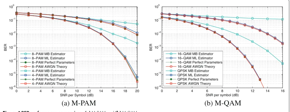
Figure 4 shows the bit-error-rate (BER) performance of the proposed algorithm. We apply the estimated chan-nel gain and interference level for symbol detection. As a comparison, the moment-based estimator is also evaluated in the simulation. It can be observed that the proposed estimator significantly outperforms the moment-based estimator in the cases of high SNR, and it shows almost the same performance as knowing the per-fect system parameters. On the other side, it also can be seen from Figure 3 and Figure 4 that the large estimation deviation of the system parameters at low SNR has little effect on the BER performance.
5 Conclusions
SNR estimation in an additive noise channel with atten-uation factor and deterministic interference has been considered. A non-data-aided iterative estimation algo-rithm has been proposed based on the ML criterion. The proposed algorithm provides satisfactory performance, although this is achieved to the price of an increased com-putational complexity. Simulation results show that the algorithm provides applicable results on the order of tens of samples. And, its performance is almost identical to the corresponding bounds over a wide range of the true SNR. Moreover, the additive noise channel of this paper also includes the case where the interference is determined by
a Gaussian random variable with non-zero mean. In this case, the interference can be divided into a constant and a zero-mean Gaussian random variable. As far as the SNR is concerned, the zero-mean Gaussian random part of the interference can be attributed to the additive Gaussian noise. Therefore, the model is also validated in this case. This case represents channels where there are many weak interferers plus noise but no dominant interferers and also represents channels where there is one dominant constant interferer plus noise. Furthermore, next step of work may focus on extending the algorithm to multipath channel environments.
Appendix
Derivations of the likelihood function for QAM signaling
∂L(r) ∂A =
N
n=1
1
H(Xn)
2p−1
i=1
(2i−1)(xn−C)
σ2 h
s i(Xn)−
(2i−1)2A
σ2 h
c i(Xn)
+
N
n=1
1
H(Yn)
2p−1
i=1
(2i−1)(yn−D)
σ2 h
s i(Yn)−
(2i−1)2A
σ2 h
c i(Yn)
= 1
σ2
N
n=1
((xn−C)Hs(Xn)+(yn−D)Hs(Yn))
− A
σ2
N
n=1
(Hc(Xn)+Hc(Yn))
(84)
∂L(r) ∂B =
N
n=1
1
H(Xn)
2p−1
i=1
(2i−1)(yn−D)
σ2 h
s i(Xn)−
(2i−1)2B
σ2 h
c i(Xn)
−
N
n=1
1
H(Yn)
2p−1
i=1
(2i−1)(xn−C)
σ2 h
s i(Yn)−
(2i−1)2B
σ2 h
c i(Yn)
= 1
σ2
N
n=1
((yn−D)Hs(Xn)−(xn−C)Hs(Yn))
− B
σ2
N
n=1
(Hc(Xn)+Hc(Yn))
∂L(r)
The authors declare that they have no competing interests.
Acknowledgements
The authors would like to thank the anonymous reviewers for their very contributive comments in making the paper more appealing. This work is supported in part by the National Natural Science Foundation of China (61372081, 61171083, 61271209), Key Grant Project of Chinese Ministry of Education (313021), Program for New Century Excellent Talents in University (NCET-12-0196) and the Fundamental Research Funds for the Central Universities of SCUT (2014ZG0028, 2014ZG0042).
Received: 27 March 2013 Accepted: 6 March 2014 Published: 25 March 2014
References
1. Y Chen, NC Beaulieu, NDA estimation of SINR for QAM signals. IEEE Commun. Lett.9(8), 688–690 (2005)
2. F Chen, F Ji, T Cao, S Xiong, Maximum likelihood based measurement of interference level and noise power for memoryless gaussian channel with deterministic interference. IEEE Trans. Commun.60(1), 19–22 (2012) 3. CH Yih, Analysis and compensation of DC offset in OFDM systems over
frequency-selective rayleigh fading channels. IEEE Trans Vehicular Technol.58(7), 3436–3446 (2009)
4. Z Wang, S Zhou, J Catipovic, P Willett, Parameterized cancellation of partial-band partial-block-duration interference for underwater acoustic OFDM. IEEE Trans. Signal Process.60(4), 1782–1795 (2012)
5. N Merhav, Universal decoding for memoryless Gaussian channels with a deterministic interference. IEEE Trans. Inform. Theory39(4), 1261–1269 (1993)
6. Y Zhao, J Wu, S Lu, Efficient SINR estimating with accuracy control in large scale cognitive radio networks, in2011 IEEE 17th International Conference on Parallel and Distributed Systems (ICPADS),(Los Alamitos, CA, USA: IEEE Computer Society, 2011), pp. 549–556
7. S Sorooshyari, CW Tan, HV Poor, On maximum-likelihood SINR estimation of MPSK in a multiuser fading channel. IEEE Trans. Vehicular Technol. 59(8), 4175–4181 (2010)
8. W Gappmair, Cramer-Rao lower bound for non-data-aided SNR estimation of linear modulation schemes. IEEE Trans. Commun.56(5), 689–693 (2008) 9. M Inamori, AM Bostamam, Y Sanada, H Minami, IQ imbalance
compensation scheme in the presence of frequency offset and dynamic DC offset for a direct conversion receiver. IEEE Trans. Wireless Commun. 8(5), 2214–2220 (2009)
doi:10.1186/1687-1499-2014-45
Cite this article as:Chenet al.:Non-data-aided ML SNR estimation for
AWGN channels with deterministic interference.EURASIP Journal on Wireless Communications and Networking20142014:45.
Submit your manuscript to a
journal and benefi t from:
7Convenient online submission 7Rigorous peer review
7Immediate publication on acceptance 7Open access: articles freely available online 7High visibility within the fi eld
7Retaining the copyright to your article