R E S E A R C H
Open Access
A semi-analytic method with an effect of
memory for solving fractional differential
equations
Kyunghoon Kim and Bongsoo Jang
**Correspondence:
[email protected] Department of Mathematical Sciences, Ulsan National Institute of Science and Technology (UNIST), Ulsan, 689-798, Republic of Korea
Abstract
In this paper, we propose a new modification of the multistage generalized
differential transform method (MsGDTM) for solving fractional differential equations. In MsGDTM, it is the key how to impose an initial condition in each sub-domain to obtain an accurate approximate solution. In several literature works (Odibatet al.in Comput. Math. Appl. 59:1462-1472, 2010; Alomari in Comput. Math. Appl.
61:2528-2534, 2011; Gökdo ˘ganet al.in Math. Comput. Model. 54:2132-2138, 2011), authors have updated an initial condition in each sub-domain by using the approximate solution in the previous sub-domain. However, we point out that this approach is hard to apply an effect of memory which is the basic property of fractional differential equations. Here we provide a new algorithm to impose the initial conditions by using the integral operator that enhances accuracy. Several illustrative examples are demonstrated, and it is shown that the proposed technique is robust and accurate for solving fractional differential equations.
1 Introduction
In recent years, fractional differential equations have been considered as an important mathematical modeling in various fields of applied sciences and engineering because of describing memory properties. Several numerical methods for solving fractional differen-tial equations have been introduced. Authors in [, ] presented the predictor-corrector approach based on the Adams-Bashforth-Moulton type numerical method that has been successful to obtain the stable approximate solutions for many fractional differential equa-tions. Some of semi-analytic methods for solving fractional problems such as the Adomian decomposition method (ADM) [–], homotopy analysis method (HAM) [–], homo-topy perturbation method (HPM) [, ], variational iteration method (VIM) [–] and generalized differential transform method (GDTM) [–] have been introduced to pro-vide analytic or numeric approximations. In this paper, we propose a new modification of multistage generalized differential transform method (MsGDTM) to obtain an accu-rate approximate solution for solving fractional differential equation. The new proposed method gives an algorithm to impose an accurate initial condition in each sub-domain which contains the effect of memory. The paper is organized as follows. Section intro-duces some definitions and notations of fractional calculus that we shall use. In Section , we present the basic ideas and some properties of GDTM. Difference between the stan-dard MsGDTM and the proposed MsGDTM are described in Section . Several numerical
illustrations are demonstrated, and they show the effectiveness of the proposed method in Section . Finally, we give a conclusion.
2 Preliminary
In this section we give some basic definitions and properties of the fractional calculus presented in this work.
Definition The Riemann-Liouville fractional integral operator of orderα≥ of a func-tionf(t)∈Cμ,t>a≥,μ≥–, is defined by
The Riemann-Liouville fractional derivative is defined by
Dα
wherem– <α≤mandm∈N. The Riemann-Liouville fractional derivative has been studied by many mathematicians. However, it is not suitable to model real world physical phenomena because it has difficulties to define the fractional order physical conditions such as initial condition. Here, we shall introduce a modified fractional differential oper-atorDα
a proposed by Caputo [].
Definition The fractional derivative in the Caputo sense off(t),f(t)∈C–m,t>a≥,
3 Generalized differential transform method
all coefficients in Taylor series can be determined by solving the recursive equation that is induced from the given differential equation. In order to apply the DTM to solve frac-tional problems, we adopt the generalized Taylor formula that was introduced in []. In what follows we describe the basic idea of the generalized differential transform method (GDTM) and its properties. Let us introduce the generalized Taylor series formula with the Caputo fractional derivative.
Theorem . (Generalized mean value theorem []) Suppose that f(t)∈C[a,b]and Dα
af(t)∈C(a,b],for <α≤,we have f(t) =f(a) +
(α)D α
af(η)(t–a)
α
with a≤η≤t for all t∈(a,b]. Let us define (Dα
a)nby
Dα
a n
=Dα
a·Dαa· · ·Dαa(n-times).
Theorem .(Generalized Taylor’s formula []) Suppose that(Dα
a)kf(t)∈C(a,b]for k=
, , . . . ,n+ ,where <α≤,then we have
f(t) =
n
i=
(t–a)iα
(iα+ )
Dα
a i
f(a) + ((D α
a)n+f)(η)
((n+ )α+ )(t–a) (n+)α
with a≤η≤t,for all t∈(a,b].
Let us define the generalized differential transform (GDT) of thekth derivative off(t) att=tas follows:
F(k) =
(αk+ )
Dαtkf(t)t=t ,
where <α≤,k= , , , . . . , and the generalized differential inverse transform ofF(k) is defined as follows:
f(t) =
∞
k=
F(k)(t–t)αk.
In case ofα= , the GDT reduces to the classical differential transform.
Theorem . Several fundamental properties of the GDT are listed below[].
. Iff(t) =g(t)±h(t),thenF(k) =G(k)±H(k).
. Iff(t) =ag(t),thenF(k) =aG(k),whereais a constant. . Iff(t) =g(t)h(t),thenF(k) =kr=G(r)H(k–r). . Iff(t) =Dα
tg(t),thenF(k) =
(α(k+)+)
(αk+) G(k+ ).
. Iff(t) = (t–t)nα,thenF(k) =δ(k–n),whereδ(k) =
. Iff(t) =Dβtg(t),m– <β≤m,then
F(k) = (αk+β+ )
(αk+ ) G
k+β
α
.
4 The multistage generalized differential transform method with an effect of memory
4.1 The standard generalized multistage differential transform method
The basic idea of multistage generalized differential transform method (MsGDTM) is to apply the standard GDTM to the given problem in each sub-domain. In order to describe the MsGDTM, let us consider the following fractional initial value problem:
Dα
ty(t) =f
t,y(t), t> ,y(t) =y. ()
In order to apply the GDTM, we assume that the solutiony(t) is expanded by the gener-alized Taylor series att=t
y(t) =
∞
k=
Y(k)(t–t)αk,
where
Y(k) =
(αk+ )
Dαtkf(t) t=t .
Some fundamental properties in Theorem . give the following recursive relation for the differential transform:
(α(k+ ) + )
(αk+ ) Y(k+ ) =F(k), k= , , , . . . , () whereF(k) is the generalized differential transform off(t,y(t)) att=t. Combined with
Y(), that is, the initial conditiony(t), the recursive equation () can be easily solved. Recalling that GDTM is based on the generalized Taylor series, an approximate solution can be obtained in a radius of convergenceR
R=|t–t|α lim
n→∞
(nα+ )
((n+ )α+ )· (Dα
t)
n+f(t)
(Dα
t)nf(t)
t=t .
In other words, it is impractical to achieve an accurate approximation by using the GDTM outside the radius of convergenceR. To overcome this difficulty, the standard GDTM is applied in each sub-domain, which is called the MsGDTM.
For the equally spaced partitionP: =t<t<· · ·<tN–<tN=T, where the nodesti=i· h,h=T/N. On theith sub-domaini≡(ti,ti+),i= , , . . . ,N– , we definey(t)|i≡yi(t)
andf(t)|i≡fi(t). The generalized differential transformYi(k) ofyi(t) att=tiis defined
by
Yi(k) =
(αk+ )
The generalized differential inverse transform ofYi(k) is defined by
yi(t) =
∞
k=
Yi(k)(t–ti)αk.
Then the generalized differential transformYi(k) is obtained by solving the following
re-cursive relation:
(α(k+ ) + )
(αk+ ) Yi(k+ ) =Fi(k), k= , , , . . . , () whereFi(k) is the generalized differential transform off(t,y(t)) att=ti. Suppose thatsi,ni
is theni-partial sum ofyi(t) ini, that is,
yi(t)≈ ni
k=
Yi(k)(t–ti)αk≡si,ni(t).
Then the solutiony(t) in () can be approximated by
y(t)≈
N–
i=
χi(t)si,ni(t),
where
χi(t) =
ift∈i,
otherwise.
In order to solve (), it is necessary to have the initial conditionyi(ti) in each sub-domain
i,i≥. Fori= , the initial condition givesY() =y(). However, there are no given initial conditionsyi(ti),i≥. In the standard multistage differential transform method
(MsDTM) for solving differential equations with integer order, the initial conditionyi(ti)
can be approximated by computingsi–,ni–(ti). In other words,Yi() =si–,ni–(ti),i≥. This approach has been successful to obtain accurate approximate solutions []. In the MsGDTM for solving fractional differential equations the same technique has been em-ployed in [, ].
4.2 Effect of memory in the standard multistage generalized differential transform method
Suppose thatyi(t) is a solution of the following problem:
Dαtiyi(t) =fi
t,yi(t)
, t∈i= (ti,ti+),i≥. ()
The analytical solution of () with an initial conditionyi(ti) can be obtained by taking the
Riemann-Liouville integral operator as follows:
yi(t) =yi(ti) +
(α)
t
ti
(t–τ)α–f
i
τ,yi(τ)
Lemma . Suppose yi(t) =
∞
k=Yi(k)(t–ti)αkand fi(t) =
∞
k=Fi(k)(t–ti)αk.Then Eq. () has the following recursive relation:
(α(k+ ) + )
standard MsGDTM finds an approximate solution of () with an initial conditionyi(ti)≈ si–,ni–(ti). Solving the recursive relation, the solutionyi(t) can be approximated byyi(t)≈
si,ni(t). Therefore it is easy to see that the standard MsGDTM approximates the value of yi(ti+) as follows:
Hence the value ofy(ti+) can be approximated by
As seen in () and (), it is clear that the standard MsGDTM is missing the memory term:
memory≡
Thus it is difficult to obtain an accurate approximation by using the standard MsGDTM for solving the fractional differential equations.
In order to avoid this difficulty, it is necessary to introduce a new algorithm to impose the memory term at each sub-domaini. Here, as described in [], we apply the piecewise
linear interpolation off(τ,y(τ)) inkatk= , , . . . ,i+ to obtain the value ofy(ti+) as
Since the approximation of yi(t) in each sub-intervali can be obtained by using the
GDTM,yi(t)≈si,ni(t), the initial conditiony(ti+) can be evaluated by
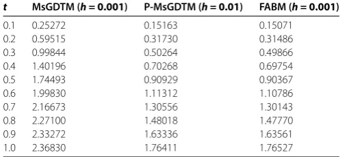
Table 1 Comparison of numerical results by the standard MsGDTM, the P-MsGDTM and the FABM forα= 0.9 in Example 1
t MsGDTM (h= 0.001) P-MsGDTM (h= 0.01) FABM (h= 0.001)
0.1 0.25272 0.15163 0.15071
0.2 0.59515 0.31730 0.31486
0.3 0.99844 0.50264 0.49866
0.4 1.40196 0.70268 0.69754
0.5 1.74493 0.90929 0.90367
0.6 1.99830 1.11312 1.10786
0.7 2.16673 1.30556 1.30143
0.8 2.27100 1.48018 1.47770
0.9 2.33272 1.63336 1.63561
1.0 2.36830 1.76411 1.76527
both the standard MsGDTM and the P-MsGDTM, the approximate solutions are obtained by using five generalized differential transforms. That is,yi(t)≈
k=Yi(k)(t–t)αk. All solutions are computed up to timet= . when the fractional orderα varies from . to ..
Example Consider the fractional Riccati equation []
Dαy(t) = y(t) –y(t) + , st> ,
where <α≤, subject to the initial conditiony() = .
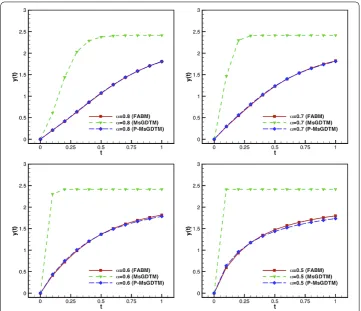
Table shows a comparison of the numerical results obtained by the standard Ms-GDTM, the P-MsGDTM and the FABM for the fractional orderα= .. The time step is chosen as h= . in the standard MsGDTM and the FABM, and h= . in the P-MsGDTM. The numerical results in the P-MsGDTM are in a good agreement with the ones in FABM at each timet= ., . . . , .. However, the standard MsGDTM gives inaccu-rate approximate solutions. Forα= ., ., . and ., the comparisons of the numerical results are shown in Figure . It is easy to see that the P-MsGDTM gives accurate numer-ical solutions for allα, but the standard MsGDTM does not. As the fractional orderα
is getting smaller, the standard MsGDTM gives an inaccurate approximate solution in a shorter range of time.
Example Consider the fractional differential equation []
Dαy(t) = –y(t),
where <α≤, subject to the initial conditionsy() = .
The exact solution can be written analytically,y(t) =Eα(–tα), whereEα(z) is the one-parameter Mittag-Leffler function as follows:
Eα(z) =
∞
k= (z)k
(αk+ ).
Figure 1 Numerical comparisons for the fractional orderα= 0.5, 0.6, 0.7 and 0.8: FABM (h= 0.001), MsGDTM (h= 0.001) and P-MsGDTM (h= 0.01) in Example 1.
Table 2 Comparison of numerical results by the standard MsGDTM, the P-MsGDTM and the exact solution forα= 0.9 in Example 2
t MsGDTM (h= 0.005) P-MsGDTM (h= 0.005) Exact solution
0.1 0.83816 0.87835 0.87809
0.2 0.70252 0.78628 0.78576
0.3 0.58883 0.70881 0.70807
0.4 0.49354 0.64201 0.64109
0.5 0.41367 0.58367 0.58261
0.6 0.34672 0.53227 0.53111
0.7 0.29061 0.48673 0.48549
0.8 0.24358 0.44618 0.44488
0.9 0.20416 0.40994 0.40859
1.0 0.17112 0.37744 0.37606
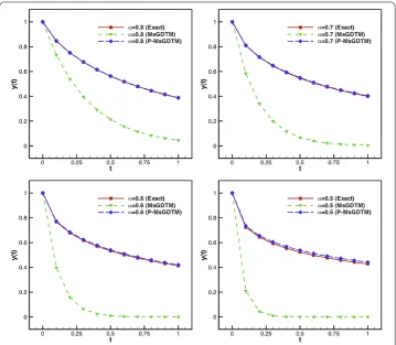
decimal places for allt. However, the standard MsGDTM gives only reliable approxima-tions when the time is close to zero and the error is getting larger as the time increases. Figure presents the comparisons of the numerical results by the standard MsGDTM and P-MsGDTM and the exact solutions for the fractional orderα= ., ., . and ..
Example Consider the following fractional differential equation:
Dαy(t) =expy(t) – y(t),
Figure 2 Numerical comparisons for the fractional orderα= 0.5, 0.6, 0.7 and 0.8: MsGDTM (h= 0.005) and P-MsGDTM (h= 0.005) in Example 2.
Table 3 Differential transformsGi(k) forg(t) = exp[y(t)],k= 0, 1, 2, 3, 4
k Gi(k)
0 exp[Yi(0)] 1 Yi(1) exp[Yi(0)]
2 ((Yi(1))2/2 +Yi(2)) exp[Yi(0)]
3 ((Yi(1))3/3! +Yi(1)Yi(2) +Yi(3)) exp[Yi(0)]
4 ((Yi(1))4/4! + (Yi(1))2Yi(2)/2! + (Yi(2))2/2 +Yi(1)Yi(3) +Yi(4)) exp[Yi(0)]
Table 4 Comparison of numerical results by the standard MsGDTM, the P-MsGDTM and the FABM forα= 0.9 in Example 3
t MsGDTM (h= 0.01) P-MsGDTM (h= 0.1) FABM solution (h= 0.001)
0.1 0.15248 0.12301 0.12229
0.2 0.28534 0.21661 0.21653
0.3 0.40432 0.29700 0.29824
0.4 0.51386 0.36926 0.37165
0.5 0.61766 0.43587 0.43916
0.6 0.71902 0.49846 0.50237
0.7 0.82132 0.55820 0.56252
0.8 0.92843 0.61608 0.62056
0.9 1.04548 0.67294 0.67735
Figure 3 Numerical comparisons for the fractional orderα= 0.5, 0.6, 0.7 and 0.8: MsGDTM (h= 0.01) and P-MsGDTM (h= 0.1) in Example 3.
Table 5 Differential transformsGi(k) forg(t) =y(t) ln[y(t)],k= 0, 1, 2, 3, 4
k Gi(k)
0 Yi(0) ln[Yi(0)] 1 Yi(1) ln[Yi(0)] +Yi(1)
2 Yi(2) ln[Yi(0)] +Yi(2) + (Yi(1))2
2Yi(0)
3 Yi(3) ln[Yi(0)] +Yi(3) +Yi(1)Yi(0)Yi(2)– (Yi(1))3 6(Yi(0))2
4 Yi(4) ln[Yi(0)] +Yi(4) +2Yi(1)Yi2(3)+(Yi(0)Yi(2))2– (Yi(0))2Yi(2)
2(Yi(0))2 +
(Yi(1))4 12(Yi(0))3
In order to obtain a recursive relation for the nonlinear term exp[y(t)], we adopted the method in [] using the Adomian polynomials. Let us assume g(t) =exp[y(t)] =
∞
k=Gi(k)(t–ti)k, then the Adomian polynomial gives the differential transformsGi(k)
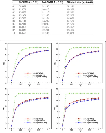
Table 6 Comparison of numerical results by the standard MsGDTM, the E-MsGDTM and the FABM forα= 0.9 in Example 4
t MsGDTM (h= 0.01) P-MsGDTM (h= 0.01) FABM solution (h= 0.001)
0.1 0.88925 0.81180 0.81250
0.2 1.19751 1.04318 1.04599
0.3 1.39697 1.21115 1.21592
0.4 1.51304 1.32935 1.33529
0.5 1.57693 1.41164 1.41800
0.6 1.61111 1.46902 1.47529
0.7 1.62911 1.50939 1.51529
0.8 1.63853 1.53817 1.54357
0.9 1.64343 1.55901 1.56389
1.0 1.64597 1.57436 1.57873
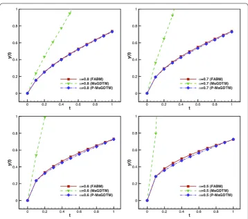
Figure 4 Numerical comparisons for the fractional orderα= 0.5, 0.6, 0.7 and 0.8: MsGDTM (h= 0.01) and P-MsGDTM (h= 0.01) in Example 4.
Example Consider the following fractional differential equation:
Dαy(t) = y(t) – y(t)lny(t),
where <α≤, subject to the initial conditionsy() = ..
For the nonlinear termln[y(t)], we obtained the differential transforms by using the Ado-mian polynomials in []. Assumingg(t) =y(t)ln[y(t)] =∞k=Gi(k)(t–ti)k, the differential
transformsGi(k) are listed in Table . For the fractional order forα= ., the numerical
(h= .) are shown in Table . Forα= ., ., . and ., the approximate solutions are depicted in Figure . Even if the numerical results by the P-MsGDTM with small frac-tional order have some difference with the results by the FABM, it will be overcome with a small time step. In fact, if we consider the numerical error forα= . att= , the error is about . forh= . but . forh= ..
6 Conclusion
In this paper, we proposed a new modified multistage generalized differential transform method for solving fractional differential equations. We have pointed out that the standard MsGDTM has difficulty to handle the effect of memory in solving fractional differential equations. However, the proposed MsGDTM (P-MsGDTM) can deal with the memory effectively. Several illustrative examples showed that the P-MsGDTM obtained accurate numerical approximations, but the standard MsGDTM failed to get robust approxima-tions for all examples. It is concluded that the proposed MsGDTM is very simple and effective for solving fractional problems. Here, all numerical results were performed by using Mathematica ..
Competing interests
The authors declare that they have no competing interests.
Authors’ contributions
BJ established the scheme, performed all the numerical examples in Section 5 and drafted the manuscript. KK helped to inspect the manuscript and designed the figures. All authors read and approved the final manuscript.
Acknowledgements
This research was supported by Basic Science Research Program through the National Research Foundation of Korea (NRF) funded by the Ministry of Education, Science and Technology (No. 2011-0004869).
Received: 13 May 2013 Accepted: 20 November 2013 Published:18 Dec 2013 References
1. Diethelm, K, Ford, NJ, Freed, D: A predictor-corrector approach for the numerical solution of fractional differential equation. Nonlinear Dyn.29, 2-22 (2009)
2. Baleanu, D, Diethelm, K, Scalas, E, Trujillo, J: Fractional Calculus Models and Numerical Methods. World Scientific, Boston (2012)
3. Saha Ray, S, Bera, RK: An approximate solution of a nonlinear fractional differential equation by Adomian decomposition method. Appl. Math. Comput.167, 561-571 (2005)
4. Hu, Y, Luo, Y, Lu, Z: Analytical solution of the linear fractional differential equation by Adomian decomposition method. J. Comput. Appl. Math.215, 220-229 (2008)
5. Duan, J-S, Rach, R, Baleanu, D, Wazwaz, A-M: A review of the Adomian decomposition method and its applications to fractional differential equations. Commun. Fract. Calc.3, 73-99 (2012)
6. Hashim, I, Abdulaziz, O, Momani, S: Homotopy analysis method for fractional IVPs. Commun. Nonlinear Sci. Numer. Simul.14, 674-684 (2009)
7. Odibat, Z, Momani, S, Xu, H: A reliable algorithm of homotopy analysis method for solving nonlinear fractional differential equations. Appl. Math. Model.34, 593-600 (2010)
8. Elsaid, A: Homotopy analysis method for solving a class of fractional partial differential equations. Commun. Nonlinear Sci. Numer. Simul.16, 3655-3664 (2011)
9. Abdulaziz, O, Hashim, I, Momani, S: Application of homotopy-perturbation method to fractional IVPs. J. Comput. Appl. Math.216, 574-584 (2008)
10. Abdulaziz, O, Hashim, I, Momani, S: Solving systems of fractional differential equations by homotopy-perturbation method. Phys. Lett. A372, 451-459 (2008)
11. Das, S: Analytical solution of a fractional diffusion equation by variational iteration method. Comput. Math. Appl.57, 483-487 (2009)
12. Guo, S, Mei, L: The fractional variational iteration method using He’s polynomials. Phys. Lett. A375, 309-313 (2011) 13. Wu, G-c: A fractional variational iteration method for solving fractional nonlinear differential equations. Comput.
Math. Appl.61, 2186-2190 (2011)
14. Wu, GC, Baleanu, D: Variational iteration method for the Burgers flow with fractional derivatives-New Lagrange multipliers. Appl. Math. Model.37, 6183-6190 (2012)
15. Wu, GC, Baleanu, D: Variational iteration method for fractional calculus - a universal approach by Laplace transform. Adv. Differ. Equ.2013, Article ID 18 (2013)
17. Odibat, Z, Shawagfeh, N: Generalized Talyor’s formula. Appl. Math. Comput.186, 286-293 (2007)
18. Odibat, Z, Momani, S, Erturk, VS: Generalized differential transform method: application to differential equations of fractional order. Appl. Math. Comput.197, 467-477 (2008)
19. Caputo, M: Linear models of dissipation whoseQis almost frequency independent. Part II. Geophys. J. R. Astron. Soc.
13, 529-539 (1967)
20. Jang, MJ, Chen, CL, Liu, YC: On solving the initial-value problems using the differential transformation method. Appl. Math. Comput.115, 145-160 (2000)
21. Jang, MJ, Chen, CL, Liu, YC: Two-dimensional differential transform for partial differential equations. Appl. Math. Comput.121, 261-270 (2001)
22. Ravi Kanth, ASV, Aruna, K: Differential transform method for solving the linear and nonlinear Klein-Gordon equation. Comput. Phys. Commun.180, 708-711 (2009)
23. Jang, B: Comments on ‘Solving a class of two-dimensional linear and nonlinear Volterra integral equations by the differential transform method’. J. Comput. Appl. Math.233, 224-230 (2009)
24. Jang, B: Solving linear and nonlinear initial value problems by the projected differential transform method. Comput. Phys. Commun.181, 848-854 (2010)
25. Odibat, Z, Bertelle, C, Aziz-Alaoui, MA, Duchamp, GHE: A multi-step differential transform method and application to non-chaotic or chaotic systems. Comput. Math. Appl.59, 1462-1472 (2010)
26. Alomari, AK: A new analytic solution for fractional chaotic dynamical systems using the differential transform method. Comput. Math. Appl.61, 2528-2534 (2011)
27. Gökdo ˘gan, A, Yildirim, A, Merdan, M: Solving a fractional order model of HIV infection of CD4+ T cells. Math. Comput. Model.54, 2132-2138 (2011)
28. Elsaid, A: Fractional differential transform method combined with the Adomian polynomials. Appl. Math. Comput.
218, 6899-6911 (2012)
10.1186/1687-1847-2013-371
Cite this article as:Kim and Jang:A semi-analytic method with an effect of memory for solving fractional differential