R E S E A R C H
Open Access
Iterative channel estimation and data
detection for MIMO-OFDM systems operating
in time-frequency dispersive channels under
unknown background noise
Ke Zhong
*, Xia Lei and Shaoqian Li
Abstract
In this paper, the challenging problem of joint channel estimation and data detection for multiple-input
multiple-output orthogonal frequency division multiplexing systems operating in time-frequency dispersive channels under unknown background noise is investigated. Based on two different but equivalent signal models, two
expectation-maximization algorithm-based iterative schemes for joint data detection and channel and noise variance estimation are proposed. The first scheme jointly detects data and estimates the channel and noise variance, but the computational complexity is high, owing to the simultaneous detection and estimation for all antennas. To reduce the computational complexity, a complexity-reduced scheme that is detecting data and estimating channel for only one antenna during each iteration and holding the unknown quantities of other antennas to their last values is proposed, whose performance only slightly degrades compared to the first scheme. Moreover, both schemes are derived as closed-form expressions, and therefore, our proposed schemes are free of exhaustive search. Simulation results demonstrate quick convergence of the proposed algorithm, and after convergence, the performance of the proposed algorithm is close to that of the optimal channel estimation and data detection case, which assumes full training and perfect channel state information.
Keywords: Multiple-input multiple-output (MIMO); Orthogonal frequency division multiplexing (OFDM); Time-frequency (TF) dispersive channels; Unknown noise variance; Expectation-maximization (EM)
1 Introduction
Multiple-input multiple-output (MIMO) communication [1] can significantly increase the throughput without increasing the transmit power and additional bandwidth. Orthogonal frequency division multiplexing (OFDM) [2] can provide high data rate transmission capabil-ity and is robust against multipath (time-dispersive) fading channels. MIMO combined with OFDM (MIMO-OFDM) [3] has been adopted in various interna-tional standards such as 3GPP-LTE, WiMAX, and IMT-Advanced.
*Correspondence: [email protected]
1National Key Laboratory of Science and Technology on Communications, University of Electronic Science and Technology of China, Chengdu 611731, People’s Republic of China
Meanwhile, vehicles with increased speeds, such as high-speed cars, subways, and trains which exceed 350 km/h, play an increasingly important role in peoples’ lives.
Consequently, mobility support is widely regarded as one of the key features in current and future wireless communication systems. High mobility causes the trans-mission channel to change rapidly in time, which results in frequency dispersion of the channel. For coherent detec-tion in MIMO-OFDM systems, channel state informadetec-tion (CSI) is indispensable [3].
CSI acquisition is particularly challenging in time-frequency (TF) dispersive channels because channel responses vary sample by sample, and therefore, the number of unknown channel parameters in an OFDM
symbol period increases significantly (much greater than in frequency-nondispersive channels). Furthermore, in practical communication scenarios, the knowledge of the power of background noise is required to per-form many signal processing algorithms, such as chan-nel estimation [4] and decoding [5] in MIMO-OFDM systems.
In this paper, joint data detection and channel and noise variance estimation for MIMO-OFDM systems operating in TF dispersive channels under unknown background noise are investigated. We employ the expectation-maximization (EM) algorithm [6,7], which is an iterative numerical method employed to com-pute the maximum likelihood (ML) estimates, to develop an iterative algorithm to solve this challenging problem.
For MIMO systems, the literature along these lines can be categorized as follows:
EM for channel estimation and data detection assuming the noise variance is known: EM-based joint channel estimation and data detection algorithms in time-nondispersive and frequency-nondispersive channels (TnDFnD channels) are proposed in [8-10], and in time-dispersive and frequency-nondispersive channels (TDFnD channels) are proposed in [11-13], respectively. However, the maximization step (M-step) for data detection proposed in these papers is not obtained as a closed-form solution, and therefore, a brute-force searching over all of the possibilities is required.
EM for channel and noise variance estimation: In TnDFnD channels, EM-based joint channel and noise variance estimation algorithms are proposed in [14-16]. However, data detection is obtained by an extra ML esti-mator and a maximizinga posterioriprobabilities (APP) detector in [14,15], respectively.
In [16], a full training sequence is adopted to perform the proposed EM algorithm, and there-fore, no data detection is addressed. In TDFnD channels, EM-based joint channel and noise vari-ance estimation algorithms are proposed in [17-19]. However, data detection is not addressed in these papers.
EM for data detection and noise variance estimation: In TnDFnD channels, an EM-based joint data detection and noise variance estimation algorithm is proposed in [20]. However, the channel estimate is only obtained by pilot symbols and is not included in the EM updating process.
EM only for data detection assuming the noise vari-ance is known: In TnDFnD channels, EM-based data detection algorithms are proposed in [21,22]. How-ever, channel estimation is not addressed in [21], and the channel knowledge is assumed ideally known at
the receiver in [22]. In TF channels, an EM-based data detection algorithm is proposed in [23] to solve a maximum a posteriori probability (MAP) detection problem. However, the data estimate is not given by a closed form, and therefore, the exhaustive search is required.
EM only for channel estimation assuming the noise vari-ance is known: In TnDFnD channels, EM-based channel estimation algorithms are proposed in [24-28]. How-ever, the data estimates are obtained by extra MAP estimators in [24-26] and APP estimators in [27,28], respectively. In TDFnD channels, EM-based channel estimation algorithms are proposed in [29-32]. How-ever, the data estimates are obtained by an extra BI-GDFE detector in [29], a minimum mean-squared error (MMSE) detector in [30], a trellises approach in [31], respectively, and data detection is not addressed in [32].
In this paper, based on two different but equiva-lent signal models, two EM algorithm-based iterative schemes which integrate data detection and channel and noise variance estimation are proposed in a con-sistent way so as to iteratively improve the system performance.
The first scheme jointly detects data and estimates the channel and noise variance, but the computational complexity is high, owing to the simultaneous detec-tion and estimadetec-tion for all antennas. To reduce the computational complexity of the first scheme, another scheme that performs data detection and channel esti-mation for only one antenna during each iteration and holding the unknown quantities of other antennas to their last values is proposed, whose performance only slightly degrades compared to the first scheme. Furthermore, the estimates of data, channel, and noise variance are all obtained as closed-form results, and therefore, the proposed schemes are free of exhaustive search. Sim-ulation results demonstrate quick convergence of the proposed algorithm, and after convergence, the per-formance of the proposed iterative algorithm is close to that of the optimal channel estimation and data detection case, which assumes full training and perfect CSI.
The remainder of this paper is organized as follows. The system model for MIMO-OFDM systems operating in TF dispersive channels under unknown background noise is introduced in Section 2.
Notation: Matrices and vectors are represented by boldface uppercase and lowercase letters, respectively.
A hat over a variable (e.g., xˆ) indicates an estimate of the variable. E{·} denotes the expectation. Super-scripts [·]T, [·]−1, and [·]H denote the transpose, the matrix inversion, and the Hermitian operations, respec-tively.IN is an identity matrix with dimensionN. diag{x} and Blkdiag{·} stand for the diagonal matrix with vec-tor x on its diagonal and the block diagonal concate-nation of input arguments, respectively. The symbol denotes convolution, and ⊗ stands for the Kronecker product. Tr{X} and |X| are the trace and the determi-nant of a square matrix X, respectively. {·}is the real part of the element in the bracket. < · >K denotes the mode K operation. The matrix F is the normal-ized fast Fourier transform (FFT) matrix with [F]m,n=
1
√ Ne
−j2πmn/N.
2 System model
2.1 Transmitted MIMO-OFDM systems with scattered pilots
We consider a MIMO-OFDM system withNT transmit andNRreceive antennas. For theith transmit antenna, the time domain signalsi =[si(0),si(1), ...,si(N−1)]Tis gen-erated by taking theN-point inverse FFT of the source signal in the frequency domainxi=[xi(0),xi(1), ...,xi(N− 1)]Tassi=FHxi.
In general, the elements ofxican be categorized into:
xi(m)=
xid(m) ∀ m∈Idi
xip(m) ∀ m∈Iip (1)
whereIdi is the index set of subcarriers allocated for data symbols (withNdelements), andIpi is the index set of sub-carriers allocated for pilot symbols (with Np elements), respectively. Notice thatN =Nd+Np. From (1), we have
xi = Ei
dxid+ Eipxpi, whereEid andEip denote the matri-ces collecting columns ofIN corresponding toIdi andIpi, respectively, andxid = [xid(0),xid(1), ...,xid(Nd−1)]T and
xip = [xip(0),xip(1), ...,xip(Np −1)]T denote the data and pilot vectors, respectively.
A cyclic prefix (CP) with length Ncp larger than that
of the longest channel response is inserted at the begin-ning of each OFDM symbol to prevent intersymbol interference.
2.2 TF dispersive channels under unknown background noise model
At the receive antennaj, assuming perfect timing and fre-quency synchronization are achieved, thenth sample of the received signal is given by:
yj(n)= NT−1
i=0
hji(n,l)si(n)+wj(n), (2)
wherehji(n,l)is the TF dispersive channel of thelth path with lengthLat timen, associated with theith transmit antenna and thejth receive antenna, andwj(n)denotes the unknown background noise and is assumed to obey com-plex Gaussian distribution with zero mean and unknown varianceσ2, which is assumed to be the same across all receive antennas.
After discarding the CP and stacking allNsamples, the received signal for a whole OFDM symbol at the receive antennajcan be expressed in a vector form as:
yj=
NT−1
i=0
Hjisi+wj, (3)
where yj = [yj(0),yj(1), ...,yj(N − 1)]T and wj =
[wj(0),wj(1), ...,wj(N − 1)]T denote the received signal at the receive antenna j and the corresponding noise, respectively.
Hjirepresents the corresponding TF dispersive channel matrix and is expressed as:
Hji= ⎡ ⎢ ⎢ ⎢ ⎢ ⎢ ⎢ ⎣
hji(0, 0) 0. . . hji(0,L−1) . . . hji(0, 1) ..
. ... . .. ...
hji(L−1,L−1) hji(L−1,L−2) . . . hji(L−1, 0) 0. . .
..
. ... . .. ...
0. . . hji(N−1,L−1) hji(N−1,L−2) . . . hji(N−1, 0) ⎤ ⎥ ⎥ ⎥ ⎥ ⎥ ⎥ ⎦
It is observed from (4) that the number of unknowns in Hji is NL, which is much larger than the num-ber of received samples. Therefore, direct estimation of
Hji is almost impossible (i.e., this will give rise to the identifiability problem).
To overcome this problem, in this paper, a parsimo-nious (low-dimensional) representation of hji(n,l) using the basis expansion model (BEM) [33,34] is adopted, i.e., using an expansion with respect to timenof each pathlof hji(n,l)into a basis{bn,q}Qq=0as:
hji(n,l)= Q
q=0
βji
q,lbn,q, (5)
whereβqji,lis theqth BEM coefficient of thelth path asso-ciated with the channel between theith transmit antenna and the jth receive antenna; bn,q is the basis that cap-tures channel time variations, andQ+1 is the number of the basis. BEM is motivated by the observation that the temporal (n) variation ofh(n,l) is usually rather smooth due to the channel’s limited Doppler spread and therefore {bn,q}Qq=0 can be chosen as a small set (i.e.,Q N) of smooth functions.
Below, two equivalent expressions for the received sig-nal will be derived, from which closed-form solution for data detection and channel estimation can be obtained, as will be shown in the following sections.
Notice that (3) can be rewritten as:
yj=
NT−1
i=0
G[si]hji+wj, (6)
whereG[si]=[diag{sics,0}, diag{sics,1}, ..., diag{sics,L−1}] with
sics,l representing cyclically shifts (cs) si by l
posi-tions and hji = [(h0ji)T,(hji1)T, ...,(hjiL−1)T]T withhjil =
[hji(0,l),hji(1,l), ...,hji(N −1,l)]T. (6) can be put into a more compact form as:
yj=G[s]hj+wj, (7)
whereG[s]=[G[s0] ,G[s1] , ...,G[sNT−1]] andhj=[(hj0)T,
(hj1)T, ...,(hj(NT−1))T]T. Using (5),hji
l can be expressed in a vector form as
hjil =Bβjil, (8)
whereB=[b0,b1, ...,bQ] withbq=[b0,q,b1,q, ...,bN−1,q]T andβjil = [β0,jil,β1,jil...,βQji,l]T. Substituting (8) into (7), we obtain:
yj=G[s](INTL⊗B)β
j+wj, (9)
where
βj=[(βj0)T,(βj1)T, ...,(βj(NT−1))T]Twithβji=[(βji
0)T,
(βji
1)T, ...,(β
ji
L−1)T]T. By stacking the received signals from
all NR receive antennas into a single vector using (9) and (3), two equivalent expressions of the received sig-nal which explicitly show the dependence of the unknown BEM coefficient and unknown signal can be obtained, respectively, as:
y=[s]β+w (10a)
=[β]s+w, (10b)
where[s]=INR⊗(G[s](INTL⊗B)),β=[(β0)T,(β1)T,
. . .,(βNR−1)T]T, [β]=[H0,H1,. . .,HNT−1] withHi = [(H0i)H,(H1i)H,. . .,(H(NR−1)i)H]H,y=[(y0)T,(y1)T,. . .,
(yNR−1)T]T, s = [(s0)T,(s1)T,. . .,(sNT−1)T]T andw = [(w0)T,(w1)T,. . .,(wNR−1)T]T. Notice that [s] repre-sents a function ofsand can be reconstructed bysthrough (6), (7), (8) and (9). Similarly, [β] represents a func-tion ofβand can be reconstructed byβ through (3), (4) and (5).
3 Iterative data detection and channel and noise variance estimation
The ML solution of all unknown quantities in (10), i.e.,
s, β, and σ2 of w, involves multidimensional searches that pose prohibitively high computational complexity. In this and the next sections, the EM algorithm is employed to iteratively compute the ML estimates, with the differ-ent accuracy versus complexity trade-offs, respectively. As will be seen, our proposed schemes provide not only com-putationally affordable but also closed-form solutions that are free of exhaustive search.
Using the EM terminology, we takeyas the incomplete data,β as the unobservable or missing data, and (σ2,s) as parameters of interest. The iterative algorithm includes two steps (the E-step and the M-step) at each iteration. In the E-step, an expectation is taken with respect toβ conditional on the observed datayand the previous esti-mates of (σ2,s), and an objective function depending only on (σ2,s) is obtained. In the M-step, through maximizing the function obtained in the E-step, the effect of channel can be compensated, and the current updated estimates of (σ2,s) can be obtained.
The two steps at thekth iteration are detailed as follows: E-step: computeQ(σ2,s| ˆσk2−1,ˆsk−1)=E{logf(y,β|σ2,s)|y, ˆ
σ2
k−1,ˆsk−1}.
M-step: solve(σˆk2,sˆk)=arg maxσ2,sQ(σ2,s| ˆσk2−1,ˆsk−1).
More specifically, for theE-step: using Bayes’s rule, we have:
f(y,β|σ2,s)=f(y|β,σ2,s)f(β), (11) where the fact thatβis independent ofsandσ2has been used. From (11), the functionQ(σ2,s| ˆσk2−1,ˆsk−1) in the E-step can be expressed as:
Q(σ2,s| ˆσ2
k−1,sˆk−1)=E{logf(y|β,σ2,s)|y,σˆk2−1,ˆsk−1}
+E{logf(β)|y,σˆk2−1,ˆsk−1}, (12)
where the second term can be ignored in the following derivations, since it is not a function of parameters of interest, i.e., not a function of (σ2,s) and therefore will not affect the following M-step. Using (10a), the likelihood functionf(y|β,σ2,s)is obtained as:
f(y|β,σ2,s)= 1
(πσ2)NRN ×exp
−σ12(y−[s]β)H(y−[s]β)
.
(13)
Substituting (13) into (12), we have:
Q(σ2,s| ˆσ2
k−1,sˆk−1)∝ −NNRlog(πσ2) −σ12yHy−2yH[s]E{β|y,σˆk2−1,sˆk−1}
+E{βHH[s][s]β|y,σˆ2
k−1,ˆsk−1}
.
(14)
Notice that the following equation holds true for any matrixAand vectorawith compatible dimension:
aHAHAa=Tr{AHAaaH}. (15)
Define the conditional mean of β in (14) as βˆk =
E{β|y,σˆk2−1,sˆk−1}, and using (15), we obtain:
Q(σ2,s| ˆσ2
k−1,sˆk−1)∝ −NNRlog(πσ2) − 1
σ2
yHy−2{yH[s]βˆk}
+Tr{H[s][s](ϒˆk+ ˆβkβˆHk)}, (16)
whereϒˆk =E{(β− ˆβk)(β− ˆβk)H|y,σˆk2−1,sˆk−1}represents
the corresponding conditional covariance matrix ofβ. It
is shown in Appendix 1 that the conditional mean and covariance matrix are approximately given by:
ˆ
βk=(H[sˆk−1][sˆk−1])−1H[sˆk−1]y, (17)
ˆ
ϒk= ˆσk2−1
H[ˆs
k−1][ˆsk−1]
−1
. (18)
M-step: in this step, we aim to maximize
Q(σ2,s| ˆσ2
k−1,sˆk−1) with respect toσ2 ands.
Differenti-ating (16) with respect tosand setting the result to zero, neglecting those irrelevant terms we have:
∂Q(σ2,s| ˆσ2 k−1,ˆsk−1) ∂s
× ∝ ∂
∂s
2{yH[s]βˆk}−Tr{H[s][s](ϒˆk+ ˆβkβˆ H k)}
.
(19)
It is noted that since (19) depends on s in an implicit way, direct maximization of (19) with respect to s is difficult since multidimensional search is required. In what follows, an alternative expression for
Q(σ2,s| ˆσ2
k−1,sˆk−1)will be derived from which a
closed-form solution for the maximizing value of s can be obtained. Since ϒˆk is a NTNR(Q+ 1)L × NTNR(Q+ 1)L Hermitian matrix, based on eigen-decomposition, we have ϒˆk = mNT=N0R(Q+1)L−1λm,kμm,kμHm,k, where
λm,k is the mth eigenvalue of ϒˆk, and μm,k is the mth eigenvector, associated with λm,k. Substituting the eigendecomposition on ϒˆk into (19) and using the two equivalent equations derived in (10a) and (10b), we have:
2{yH[s]βˆk} −Tr{H[s][s](ϒˆk+ ˆβkβˆ H k)} =yH[βˆk]s+sHH[βˆk]y−
NTNR(Q+1)L−1
m=0
λm,ksHH[μm,k] ×[μm,k]s−sHH[βˆk][βˆk]s.
(20)
Notice that[·] and[·] defined in (10a) and (10b) are not only applicable tosandβbut also applicable to any vectors with compatible dimension.
Since (20) is a quadratic form ofs, by setting the first derivative of (20) with respect tosto zero, thekth signal estimate is then given by:
˜
sk= ⎛
⎝NTNR(Q+1)L−1 m=0
λm,kH[μm,k][μm,k]
+H[βˆ k][βˆk]
⎞ ⎠
−1
H[βˆ
Note thats˜k=[(s˜0k)T,(s˜1k)T, ...,(˜sNT−1
k )T]T. After OFDM demodulation, the symbol from theith transmit antenna can be obtained as:
˜
xik =F˜sik. (22)
Since x˜ik is discrete, belonging to a symbol constella-tion point, it must be quantized to its nearest constellaconstella-tion point in each iteration. Consequently, constellation map-ping is carried out to obtain the discrete symbol estimate as:xˆik=Qant{˜xik}, where Qant{·}operation denotes quan-tization on the element in the bracket. The data symbol estimate is thus obtained by collecting the elements ofxˆik
corresponding toIdi.
Finally, puttingˆsik =FHxˆik,i =0, 1, ...,NT−1 into (16) and setting the first derivative ofQ(σ2,s| ˆσk2−1,ˆsk−1)with respect to σ2 to zero, thekth estimate of the unknown noise variance can be obtained as
ˆ
In summary, starting from a suitable initial value, the proposed iterative EM-based scheme alternates among the explicitly closed-form results (17), (18), (21), (22), and (23) until convergence, i.e., until no significant changes are observed in the updates.
4 A reduced computational complexity scheme The computational complexity of the EM-based itera-tive scheme proposed in Section 3 is summarized in Table 1. Notice that the computational burden mainly comes from the joint detection and estimation simultane-ous for all transmit antennas. If in each iteration, detec-tion, and estimation can be completed one antenna by one antenna, the computational burden will be significantly reduced.
Table 1 Computational complexity of the proposed scheme in Section 3
Computation Complexity
Matrix inversion in (17) O((NTNR(Q+1)L)3)
Eigendecomposition on (18) O((NTNR(Q+1)L)3)
Matrix inversion in (21) O((NTN)3)
Recalling (6) and (3), two alternating but equivalent expressions forycan be derived as:
y=[s]β+w= channel from the transmit antenna i to NR receive antennas is represented by βirc = [(β0i)T,(β1i)T, ...,
The subscript ‘rc’ is short for ‘reduced complexity’ to distinguish it from the βj defined in Section 3, which represents the BEM coefficients associated with the channel from NT transmit antennas to the receive antennaj.
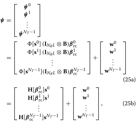
From (24a) and (24b), it is observed that by applying the mathematical framework of EM, an alternative way to choose the complete data, defined asψ in this scheme, is by decomposing the observed data y into its signal components. The complete dataψis obtained as:
ψ= symmetric and statistically independent Gaussian vectors satisfyingw=NT−1
Similar to the E-step in Section 3, for the kth itera-tion, we need to compute the conditional expectation of the log-likelihood function for the complete dataψ. More specifically, for the
E-step: using (25a), the likelihood function can be expressed as: negative and real-valued scalars satisfyingNT−1
i=0 ςi=1, = [([s0](INRL ⊗B)β0rc)T,([s1](INRL ⊗B)β1rc)T, ...,
([sNT−1](I
NRL ⊗ B)βrcNT−1)T]T. Notice that in this
scheme, we take (βrc,s) as parameters of interest. Using (26) and neglecting those irrelevant terms,
E{logf(ψ|βrc,s)|y,βˆrc,k−1,sˆk−1}can be expressed as:
ponents into the right-hand side of (28), after some manipulations we obtain:
Substituting (29) into (28), finally we obtain:
E{logf(ψ|βrc,s)|y,βˆrc,k−1,sˆk−1}
It is noted from (30) that in the following M-step, the maximization ofE{logf(ψ|βrc,s)|y,βˆrc,k−1,sˆk−1}with
respect to βrc and s is equivalent to the minimization of each of the single terms in (30), i.e., minimization of
(ψˆik−[si](INRL⊗B)β
Setςi=1, for theith transmit antenna we have:
Using (34) and (35), (30) can be decomposed intoNT terms, each of which can be solved as follows:
M-step: for theith transmit antenna, we have:
Therefore, the proposed iterative scheme starts from k = 0, 1, 2, ... and during thekth iteration,iis set asi =
<k >NT. It can be seen that we have split the estimation and detection problem for the MIMO case of Section 3 into estimation and detection problem forNTsingle-input and multiple-output (SIMO) cases, where, during each iteration, parameters and data from only one transmit antenna are estimated and detected. Note that χik given in (33) is a disturbance term that accounts for the back-ground noise and residual interference after thekth iter-ation, where the interference is linearly related to the sig-nals of all transmit antennas. Then, assuming the interfer-ence is i.i.d with zero mean, from the central limit theorem [35], it can be seen that the entries ofχikare nearly Gaus-sian distributed with zero mean and some varianceσχ2i,k. Under the above assumption, it turns out that the mini-mization problem in (36) is equivalent to the ML estima-tion ofβirc,siand the unknown varianceσχ2istarting from the observationψˆi. Comparing (34a) and (34b) with (10a) and (10b), it is easy to see that the same EM procedure proposed in Section 3 can be directly adopted to solve the optimization problem of (36), with details shown in Appendix 2.
The computationally feasible EM scheme is summarized as follows:
Iteration until convergence:
forthekth iterationdo
Setthe transmit antenna asi=<k>NT (assume the convergence occurs at theLth iteration):
forthelth iterationdo Updatingβircandϒirc:
3.Set[βˆirc,k,ˆski,σˆχ2i,k]= [βˆ i
rc,k−1,L,ˆsik−1,L,σˆχ2i,k−1,L]for the transmit antenna i.
Set[βˆgrc,k,sˆgk,σˆχ2g,k]=[βˆ g rc,k−1,sˆ
g
k−1,σˆχ2g,k−1] for the transmit antennas{g}NT−1
g=0,g =i.
end for
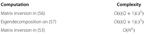
The computational complexity of the proposed iter-ative EM-based scheme with reduced complexity is summarized in Table 2.
Note that compared to Table 1, the computational com-plexity of the proposed iterative EM-based scheme with reduced complexity is significantly lower than that of the EM-based scheme proposed in Section 3. However, this significant computational complexity reduction is not obtained without price. As will be shown in Section 5, there is a minor performance degradation compared to the EM-based scheme proposed in Section 3. This per-formance degradation is due mainly to two reasons. First, the disturbance term in (34a) and (34b) contains the back-ground noise as well as the residual interference from other transmit antennas, whereas in (10a) and (10b), only the background noise is contained. Second, the separate estimation and detection for each antenna is seen as a suboptimal estimation and detection method compared to the joint estimation and detection for all antennas, which is optimal in the sense of estimation and detection theory [36].
4.1 Initialization
The EM algorithm is guaranteed to obtain at least a local maximum after convergence [6,7].
To provide an initial value, a least square (LS) algorithm based on pilot symbols is utilized to provide a good initial estimate which will be demonstrated in the simulations. Recalling (1), (10a), and (10b), we have:
y=[ pxp]β+[β] dxd+w, (38)
where p = Blkdiag{FHE0p,FHE1p, ...,FHENpT−1}, d = Blkdiag{FHE0d,FHE1d, ...,FHENT−1
d },xp = [(xp0)T,(x1p)T, ...,
(xNT−1
p )T]T, and xd = [(x0d)T,(xd1)T, ...,(xdNT−1)T]T. By
Table 2 Computational complexity of the proposed scheme in Section 4
Computation Complexity
Matrix inversion in (56) O(((Q+1)L)3)
Eigendecomposition on (57) O(((Q+1)L)3)
Matrix inversion in (53) O(N3)
treating the term containing xd as interference, the LS estimate ofβis obtained as:
ˆ
β0=
H[
pxp][ pxp] −1H
[ pxp]y. (39)
Substituting (39) into (10b), the initial signal detection is obtained as:
ˆ
s0=(INT⊗F H)Qant
(INT⊗F)
H[βˆ
0][βˆ0]
−1
×H[βˆ
0]y
.
(40)
Finally, for the initial variancesσˆ02and{ ˆσχ2i,0} NT−1 i=0 , they
are all set to 0.
5 Simulation results and discussions
In this section, the performance of the proposed algo-rithm is demonstrated by Monte Carlo simulations. In the simulations, transmit and receive antennas are set as NT = NR = 2, each OFDM symbol has 64 subcarriers (N=64) and communicates over a bandwidth of 20 MHz. The sampling intervalTsis thus 50 ns. The length of the CP isNcp=8.
The normalized maximal Doppler shift is set asNfdTs= 0.075 and 0.15, respectively, wherefdrepresents the max-imum Doppler frequency.
The channel has three taps (L = 3) with an exponen-tial power delay profile, namely σl2 = exp(−κl)((1 − exp(−κ))/(1−exp(−κL))),l=0, 1, ...,L−1 withκ=1/3. In typical communication scenarios, only a few signifi-cant paths dominate the effect of the wireless channel [4]. Therefore, L = 3 is a reasonable setting. Each tap coefficient follows a complex Gaussian distribution. The data are modulated by quadrature phase shift key-ing (QPSK) and 16 quadrature amplitude modulation (16 QAM), respectively, with unit power. The pilot clus-ter follows the structure in [37], and more specifically, seven pilot clusters are used for each transmit antenna. The clusters are equal-spaced among subcarriers, and in each cluster, one nonzero pilot is guarded by one zero pilot on each side. The nonzero pilots are generated as zero-mean complex Gaussian random variables with power three times that of data symbols. Furthermore, the gen-eralized complex exponential BEM (GCE-BEM) [34] is adopted.
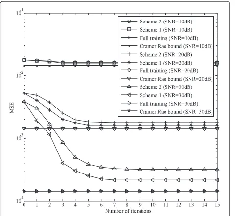
5.1 Convergence of the proposed schemes
Figure 1Convergence of channel estimation, QPSK,
NfdTs=0.075.Convergence performance of the proposed EM-based scheme in Section 3 (marked as scheme 1) and the proposed EM-based scheme in Section 4 (marked as scheme 2) with signal-to-noise ratio (SNR) equal to 10, 20, and 30 dB.
first few iterations and converge to stable values within eight iterations. Channel estimation with full training and data detection with perfect CSI are shown for compar-ison. Furthermore, according to [38], the Cramer-Rao bound is also shown for comparison. It can be seen
Figure 2Convergence of data detection, QPSK,NfdTs=0.075. Convergence performance of the proposed EM-based scheme in Section 3 (marked as scheme 1) and the proposed EM-based scheme in Section 4 (marked as scheme 2) with signal-to-noise ratio (SNR) equal to 10, 20, and 30 dB.
Figure 3Convergence of data detection, QPSK,NfdTs=0.15. Convergence performance of the proposed EM-based scheme in Section 3 (marked as scheme 1) and the proposed EM-based scheme in Section 4 (marked as scheme 2) with signal-to-noise ratio (SNR) equal to 10, 20, and 30 dB.
from Figure 1 that after convergence, the channel esti-mation performance of both schemes greatly improve that of the initial estimation (marked as iteration = 0), which indicates the ability of the proposed algorithm to cancel the interference from unknown data to channel estimation through iterations. The channel estimation performance of scheme 1 is very close to that of the Cramer-Rao bound and the full training case. The chan-nel estimation performance of scheme 2 suffers a minor performance degradation compared to that of the scheme 1, which is the price we have to pay for the reduced com-putational complexity. Similar results can be observed for the performance of data detection in Figures 2 and 3, which indicates that the updated channel estimate can in turn greatly improve the data detection through iter-ations. Similar convergence results are also observed for the 16 QAM case, and figures are not presented here due to space limitations.
5.2 Performance of the proposed schemes
Figures 4, 5, and 6 show the MSE and BER performance achieved by the proposed iterative algorithm versus SNRs. It can be seen from Figure 4 that the performances of the proposed schemes 1 and 2 both perform much better than that of the initial value and close to that of the Cramer-Rao bound and the full training case after convergence.
Figure 4Performance of channel estimation, QPSK,
NfdTs=0.075.MSE performance achieved by the proposed iterative algorithm versus SNRs.
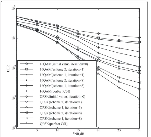
case which assumes perfect CSI after convergence. For the severe case whereNfdTs = 0.15, it can be seen from Figure 6 that the proposed iterative algorithm can still deal with such a highly TF dispersive channel and performs well. Moreover, from Figures 5 and 6, it can be seen that for signals with both amplitude and phase variations such as 16 QAM, the proposed algorithm also performs well.
Figure 5Performance of data detection, QPSK and 16 QAM,
NfdTs=0.075.BER performance achieved by the proposed iterative algorithm versus SNRs.
Figure 6Performance of data detection, QPSK and 16 QAM,
NfdTs=0.15.BER performance achieved by the proposed iterative algorithm versus SNRs.
Finally, we investigate how the proposed schemes are affected by different channel lengths. A severe case where the channel length is equivalent to the number of embedded pilots (marked as case 2) is shown in Figure 7. As can be seen from the figure, compared to the originally-presented case where the channel length is 3 (marked as case 1), there is an obvious
performance degradation of the proposed schemes for the severe case 2. The reason can be explained according to the estimation theory [36] that when the channel length increases, more parameters need to be estimated, which leads to a decreased performance. On the con-trary, if the channel length decreases, less parameters need to be estimated and that leads to an increased performance.
6 Conclusions
In this paper, two EM-based iterative data detection and channel and noise variance estimation schemes for MIMO-OFDM systems operating over TF disper-sive channels under unknown background noise have been proposed. The resulting schemes achieve conver-gence in a few iterations and can effectively estimate TF dispersive channels and obtain reliable data detec-tion under unknown background noise environments. The first scheme iteratively detects data and estimates the channel and noise variance simultaneously for all anten-nas, and moreover, the updating expressions of these esti-mates are all derived as closed-form results. Simulation results showed that after convergence, the performance of the first scheme is very close to that of the optimal case which assumes full training and perfect CSI. To reduce the computational complexity of the first scheme, another EM-based scheme that detecting data and estimating channel for only one antenna during each iteration and holding the unknown quantities of other antennas to their last estimates has been proposed, which is also derived as closed-form results. Simulation results showed that its performance only slightly degrades compared to the first scheme, but the computational complexity is significantly reduced.
Appendices Appendix 1
Derivation of (17) and (18)
Using Bayes’s formula, the conditional pdf ofβis given by:
f(β|y,σˆk2−1,ˆsk−1)=
f(y|β,σ2,s)f(β) f(y|σ2,s)
$$ $$
σ2= ˆσ2
k−1,s=ˆsk−1
,
(41)
where the fact that β is independent of s, and σ2 has been used. The BEM coefficientβ can be shown to be complex Gaussian variable [33] with zero mean and covariance matrixRβ, that is:
f(β)= 1
π(Q+1)NTNRL|Rβ|exp(−β HR−1
β β). (42)
Note that:
f(y|σ2,s)= %
f(y|β,σ2,s)f(β)dβ. (43) Withf(y|β,σ2,s)given by (13), putting (13) and (42) into (43), we have:
f(y|σ2,s)= | ˆϒk|
(πσ2)NNR|Rβ| ×exp− 1
σ2(y
Hy−σ2βˆH
kϒˆ −1
k βˆk)
. (44)
Substituting (13), (42), and (44) into (41), after some manipulations we have:
f(β|y,σˆk2−1,sˆk−1)= 1
π(Q+1)NTNRL| ˆϒ k|
×exp−(β− ˆβk)Hϒˆ−k1(β− ˆβk), (45)
where
ˆ
βk=
H[ˆs
k−1][sˆk−1]+ ˆσk2−1R−β1
−1H[ˆs k−1]y,
(46) ˆ
ϒk= ˆσk2−1
H[ˆs
k−1][ˆsk−1]+ ˆσk2−1R−β1 −1
. (47)
Thus, the pdf f(β|y,σˆk2−1,sˆk−1) is a Gaussian distri-bution. In addition, βˆk and ϒˆk given in (46) and (47), respectively, are in fact its conditional mean and covari-ance. To show that we have no prior information onβ, we take the limit||Rβ|| → +∞, which leads to (17) and (18).
In this paper, we setR−β1to zero to show we have no prior information for β. Indeed, there will be a performance degradation by assumingR−β1to zero. However, this is a typical complexity versus performance trade-off. More-over, as can be seen from simulation results in Section 5, even we set R−β1to zero, the proposed algorithm also performs well, and its performance is acceptable.
Appendix 2
Solving (36)
Comparing (34a) and (34b) with (10a) and (10b), referring to Section 3, we takeψˆikas the incomplete data,βircas the unobservable or missing data, and (σ2
χi,si) as parameters of interest. The two steps at thekth iteration are detailed as follows:
E-step: compute Q(σχ2i,si| ˆσχ2i,k−1,ˆsik−1) = E{logf(ψˆ i k,
βi
rc|σχ2i,si)| ˆψ i
k,σˆχ2i,k−1,ˆsik−1}. M-step: solve(σˆ2
χi,k,ˆsik)=arg maxσ2 χi,siQ(σ
2
χi,si| ˆσχ2i,k−1, ˆ
Note that conditioned uponψˆik, the only unknown or random component in the complete data(ψˆik,βirc)isβirc, the expectation is taken with respect to the conditional probability density functionf(βirc| ˆψik,σˆχ2i,k−1,ˆsik−1), while
(σˆ2
χi,k,ˆsik)are the estimates ofσχ2i, andsiat thekth itera-tion. More specifically, for theE-step: Using Bayes’s rule, we obtain:
where the second term can be ignored in the following derivations, since it is not a function of parameters of interest, i.e., not a function of (σχ2i,si). Using (34a), the
Substituting (50) into (49) and referring to (14), (15) and (16) and Appendix 1, the conditional mean and covariance matrix are obtained as:
M-step: using the two equivalent expressions derived in (34a) and (34b) and similar to (19), (20), (21) and (22), the signal updating equation is obtained as:
˜ resents the eigendecomposition ofϒˆirc,k. It is noted that compared to (21) whereNTN×NTNmatrix inversion is required, onlyN×Nmatrix inversion is needed in (53). The symbol detection can thus be obtained after OFDM demodulation as
ˆ
xik=Qant{F˜sik}. (54)
Substitutingˆsik =FHxˆikand (50), (51) and (52) into (49) and referring to (23), the unknown noise variance for the disturbance termχikcan be obtained as:
ˆ
In summary, (51), (52), (53), (54) and (55) solve the minimization problem in (36).
Notice that the computational complexity can be further reduced by observing the diagonal structure of both[si] and(INRL⊗B)in (24a). Therefore, (51) and (52) can be fur-ther split intoNRsub-matrices, each of which is expressed as: and (52) and therefore only N1
Competing interests
The authors declare that they have no competing interests.
Acknowledgements
This work was supported in part by the National Science Foundation of China under grant number 61032002, 60902026, and 60972029, the Chinese Important National Science & Technology Specific Projects under grant 2011ZX03001-007-01, and the Program for New Century Excellent Talents in University, NCET-11-0058.
Received: 10 December 2012 Accepted: 15 June 2013 Published: 6 July 2013
References
1. H Bocskei, AJ Paulraj,Multiple-Input Multiple-Output (MIMO) Wireless Systems (Cambridge Univ. Press, Cambridge, 2003), pp. 1–22
2. RV Nee, R Prasad,OFDM for Wireless Multimedia Communications (Artech House Publishers, Norwood, 2000), pp. 1–284
3. L Hanzo, J Akhtman, M Jiang, L Wang,MIMO-OFDM for LTE, WiFi and WiMAX: Coherent versus Non-coherent and Cooperative Turbo Transceivers
(Wiley, Hoboken, 2010), pp. 1–692
4. A Goldsmith,Wireless Communications(Cambridge Univ. Press, Cambridge, 2005), pp. 1–672
5. AJ Viterbi, JK Omura,Principles of Digital Communication and Coding (Dover Press, New York, 2009), pp. 1–576
6. AP Dempster, NM Laird, DB Rubin, Maximum likelihood from incomplete data via the EM algorithm. J. Royal Statiscal Soc., Ser. B (Methodological).
39(1), 1–38 (1977)
7. T Moon, The expectation-maximization algorithm. IEEE Signal Process. Mag.13(6), 47–60 (1996)
8. A Assra, W Hamouda, A Youssef, EM-based joint channel estimation and data detection for MIMO-CDMA systems. IEEE Trans. Veh. Technol.59(3), 1205–1216 (2010)
9. J Choi, An EM based joint data detection and channel estimation incorporating with initial channel estimate. IEEE Commun. Lett.12(9), 654–656 (2008)
10. C Cozzo, BL Hughes, Joint channel estimation and data detection in space-time communications. IEEE Trans. Commun.51(8), 1266–1270 (2003) 11. X Zhang Y, DG Wang, JB Wei, inIEEE Wireless Communications and
Networking Conference, vol. 3. Joint symbol detection and channel estimation for MIMO-OFDM systems via the variational bayesian EM algorithm (Las Vegas, 31 Mar–3 Apr 2008), pp. 13–17
12. DKC So, RS Chen, Iterative EM receiver for space-time coded systems in MIMO frequency-selective fading channels with channel gain and order estimation. IEEE Trans. Wirel. Commun.3(6), 1928–1935 (2004) 13. B Lu, X Wang, Y Li, Iterative receivers for space-time block coded OFDM
systems in dispersive fading channels. IEEE Trans. Wirel. Commun.1(2), 213–225 (2002)
14. A Zia, JPR Reilly, J Manton, S Shiran, An information geometry approach to ML estimation with incomplete data: application to semiblind MIMO channel identification. IEEE Trans. Signal Process.55(8), 3975–3985 (2007) 15. MA Khalighi, JJ Boutros, Semi-blind channel estimation using EM
algorithm in iterative MIMO APP detectors. IEEE Trans. Wirel. Commun.
5(11), 3165–3173 (2006)
16. CH Aldana, E de Cardevalho, J Ciof, Channel estimation for multicarrier multiple input single output systems using the EM algorithm. IEEE Trans. Signal Process.51(12), 3280–3292 (2003)
17. J Zhang, L Hanzo, X Mu, Joint decision-directed channel and noise-variance estimation for MIMO OFDM/SDMA systems based on expectation-conditional maximization. IEEE Trans. Veh. Technol.60(5), 2139–2151 (2011)
18. J Choi, An EM-based iterative receiver for MIMO-OFDM under interference-limited environments. IEEE Trans. Wirel. Commun.6(11), 3994–4003 (2007)
19. X Wautelet, C Herzet, A Dejonghe, J Louveaux, L Vandendorpe, Comparison of EM-based algorithms for MIMO channel estimation. IEEE Trans. Commun.55(1), 216–226 (2007)
20. I Nevat, GW Peters, J Yuan, Detection of gaussian constellations in MIMO systems under imperfect CSI. IEEE Trans. Commun.58(4), 1151–1160 (2010) 21. C Georghiades, J Han, Sequence estimation in the presence of random
parameters via the EM algorithm. IEEE Trans. Commun.45(3), 300–308 (1997)
22. F Chan, J Choi, Neighborhood exploring detector: an EM-based signal detector for multiple antenna systems. IEEE Trans. Signal Process.55(5), 1875–1885 (2007)
23. T Kashima, K Fukawa, H Suzuki, Adaptive MAP receiver via the EM algorithm and message passings for MIMO-OFDM mobile communications. IEEE J. Sel. Areas Commun.24(3), 437–447 (2006) 24. Y-L Ueng, Y-M Chen, J-Y Lin, A MIMO-BICM scheme using a convolutional
interleaver for delay-sensitive applications. IEEE Trans. Veh. Technol.59(5), 2380–2393 (2010)
25. M Khalighi, S Bourennane, Semiblind single-carrier MIMO channel estimation using overlay pilots. IEEE Trans. Veh. Technol.57(3), 951–1956 (2008)
26. J Choi, MIMO-BICM iterative receiver with the EM based channel estimation and simplified MMSE combining with soft cancellation. IEEE Trans. Signal Process.54(8), 3247–3251 (2006)
27. J Zheng, B Rao, LDPC-coded MIMO systems with unknown block fading channels: soft MIMO detector design, channel estimation, and code optimization. IEEE Trans. Signal Process.54(4), 1504–1518 (2006) 28. MA Khalighi, J Boutros, J-F H´elard, Data-aided channel estimation for
turbo-PIC MIMO detectors. IEEE Commun. Lett.10(5), 350–352 (2006) 29. T-H Pham, Y-C Liang, A Nallanathan, A joint channel estimation and data
detection receiver for multiuser MIMO IFDMA systems. IEEE Trans. Commun.57(6), 1857–1865 (2009)
30. J Gao, H Li, Low-complexity MAP channel estimation for mobile MIMO-OFDM systems. IEEE Trans. Wirel. Commun.7(3), 774–780 (2008) 31. RD Souza, J Garcia-Frias, A Haimovich M, Semiblind EM based iterative
receivers for space-time-coded modulation and quasi-static frequency-selective fading channels. IEEE Trans. Veh. Technol.55(4), 1259–1268 (2006)
32. YZ Xie, CN Georghiades, Two EM-type channel estimation algorithms for OFDM with transmitter diversity. IEEE Trans. Commun.51(1), 106–115 (2003)
33. X Ma, G Giannakis B, S Ohno, Optimal training for block transmissions over doubly selective wireless fading channels. IEEE Trans. Signal Process.
51(5), 1351–1366 (2003)
34. Z Tang, G Leus, RC Cannizzaro, P Banelli, Pilot-assisted timevarying channel estimation for OFDM systems. IEEE Trans. Signal Process.55(5), 2226–2238 (2007)
35. H Stark, JW Woods,Probability and Random Processes with Applications to Signal Processing Prentice Hall(Prentice-Hall, Upper Saddle River, 2002), pp. 1–699
36. SM Kay,Fundamental of Statistical Signal Processing: Estimation Theory (Prentice-Hall, Upper Saddle River, 1993), pp. 1–625
37. A Kannu, P Schniter, Design and analysis of MMSE pilot-aided cyclic-prefixed block transmissions for doubly selective channels. IEEE Trans. Signal Process.56(3), 1148–1160 (2008)
38. H Tree, K Bell,Bayesian Bounds for Parameter Estimation and Nonlinear Filtering/Tracking(Wiley-IEEE Press, New York, 2007), pp. 1–951
doi:10.1186/1687-1499-2013-182