R E S E A R C H
Open Access
Data quality analysis and cleaning strategy
for wireless sensor networks
Hongju Cheng
1,2*, Danyang Feng
1, Xiaobin Shi
1and Chongcheng Chen
2Abstract
The quality of data in wireless sensor networks has a significant impact on decision support, and data cleaning is an effective way to improve data quality. However, if the data cleaning strategies are not correctly designed, it might result in an unsatisfactory cleaning effect with increased system cleaning costs. Initially, data quality evaluation indicators and their measurement methods in wireless sensor networks were introduced. We then explored the impact of relationship between different indicators which are used in the quality assessment. Finally, data cleaning strategy for wireless sensor networks based on the relationship between data quality indicators was proposed by comparing and analyzing data cleaning schemes with different orders. The experimental results showed that the proposed data cleaning strategy can effectively improve data availability and have a better cleaning effect in wireless sensor networks for the same cleaning cost.
Keywords:Wireless sensor networks, Data quality, Data cleaning
1 Introduction
In wireless sensor networks (WSNs), many errors occur among the sensor data due to characteristics, such as low-cost sensors, limited resources, and link variation [1]. These errors appear in different modes, for example, the data loss or anomalies caused by hardware, the data failure due to transmission delays, and the sampling jitter [2] caused by the node task conflicts. The dataset collected by the sink node may simultaneously result in these aforementioned errors.
The data-centric feature is becoming increasingly prominent with wireless sensor networks that are widely deployed in the real world. Data is the bridge between the network and the physical world, and the quality of data has an important impact on the application. However, the dataset is not reliable due to numerous data errors in the network. It is necessary to improve the data quality to support various applications [3].
There are two main aspects of data management in wireless sensor networks, data quality assessment and data cleaning technology. The current mainstream oper-ation is to decompose the data quality into specific data
quality indicators [4] such as accuracy, timeliness, com-pleteness, and consistency [5]. There are dozens of met-rics currently used to assess the quality of sensory data, but the search for a common and valid data quality assessment framework is still ongoing. Data cleaning aims at how to detect and eliminate data errors origi-nated from the initial data [6]. The current data cleaning strategies generally deal with repeated object detection, outlier value detection, and missing data processing. Duplicate object detection finds whether there is a data duplication or inconsistency, or other issue based on the data volume and consistency indicators. Abnormal data detection aims at identifying and correcting the abnor-mal data. Elimination of sample jittering is mainly used for the time-related indicators, while missing data pro-cessing for data integrity indicators.
There are relations among different quality indicators in data cleaning. Fan et al. [7] shows that data quality in-dicators are not completely isolated. Although the data cleaning strategy might be designed for a given indicator, it may influence another indicator at the same time. For example, the cleaning of missing data mending may lead to uncertain changes in the accuracy measurement of the data when improving the integrity, due to the fact that the related cleaning technologies cannot guarantee data correctness [8]. For abnormal data correction, the
* Correspondence:[email protected]
1College of Mathematics and Computer Science, Fuzhou University, Fuzhou
350108, China
2Key Laboratory of Spatial Data Mining and Information Sharing, Ministry of
Education, Fuzhou, China
data correctness can be improved without changing the measurement of data integrity indicators. However, the current research works are less concerned with the im-pact of the relationship between various quality indica-tors, and systematic studies on the relationship between quality indicators in wireless sensor networks are still an interesting issue.
When cleaning the dataset with different problems mentioned in the first paragraph, the unsuitable cleaning sequence might not obtain the expected effect. At the same time, repeated and poor cleaning will reduce the cleaning efficiency. For example, data cleaning which aims at improving the accuracy may result in lower data-set correctness due to the abnormality of repaired data, and finally, the correct cleaning may have to be repeated. Therefore, a proper data cleaning strategy is particularly important to improve the cleaning efficiency and clean-ing effect in wireless sensor networks. At present, the issue of data cleaning instruction solutions for informa-tion system databases has been studied [8]. This paper studies the impact of relationship between different indi-cators on the quality assessment during data cleaning. By comparing and analyzing data cleaning solutions in different orders, a cleaning strategy based on the rela-tionship between data quality indicators is proposed, which can effectively improve the cleaning efficiency. The main contributions of this paper are as follows:
(1).We introduce four indicators for the data quality assessment: amount of data, correctness,
completeness, and time correlation index measure. We also provide detailed measurement for the relationship between different indicators. (2). By utilizing the relationship among different
indicators, we study the final result of different order of cleaning strategy by theoretical analysis.
(3). An efficient data cleaning strategy is proposed to solve the multiple mixed errors in wireless sensor networks, and its effect is verified by experiments.
The paper is organized as follows. In Section 2, we present the related works.Section 3describes the system model and the problem formulation. InSection 4, we de-scribe the measurement of quality indicators. InSection 5, we introduce the method including the relationship between indicators and the proposed cleaning strategy. Section 6 presents simulation results, and Section 7 is conclusion.
2 Related works
There are a large number of researches on data quality or data assessment. Data quality is usually divided into differ-ent indicators, i.e., accuracy, completeness, and timeliness [4]. In order to avoid the “dirty” data, Klein et al. [5]
propose five measures to evaluate the quality of sensor data flow, namely, accuracy, credibility, integrity, data vol-ume, and timeliness. A flexible model that presents data quality dissemination and processing is used to capture, process, and deliver quality features and provide corre-sponding business tasks. Li et al. [6] define the metrics and observe real-world data by the use of three commonly used indicators: timeliness, availability, and effectiveness. The definition of these indicators ensures that their pa-rameters are interpretable and are obtained by analyzing historical data.
Currently, there are a lot of available works regarding data cleaning. Ghorbel et al. [9] propose a method of detecting outliers by using Mahalanobis distance based on kernel principal component analysis (KPCA). KPCA calculates the mappings of data points and maps the data to another feature space, thus separates the excep-tion points from the normal data distribuexcep-tion patterns. Experiments show that KPCA performs well in detecting abnormal values and can obtain the abnormal values quickly and effectively. Zhuang et al. [10] propose a method of clearing the network outlier values. It is based on the correction of outlier values of wavelet and distance-based DTW (dynamic time warp) outlier. The cleaning process is completed during the multi-hop data forwarding process and the neighbor relationship in the hop-based routing algorithm. Experiments show that this method can clean the abnormal sensing data.
Hamrani et al. [11] use the radial basis function as the basic interpolation function to carry out the data restor-ation in WSN. Li et al. [12] propose a kd-tree based K-nearest neighbor (KNN) data restoration algorithm that uses weighted variance and weighted Euclidean dis-tance to construct a binary search tree fork-dimensional non-missing data. The size of the weight is inversely proportional to the amount of data loss of the indicator and is proportional to the variance of the indicator. For time-dependent sampling jitter, Rahm et al. [13] aim at eliminating the non-uniform sampling time series and propose to eliminate the data error by using linear interpolation. During the execution of the algorithm, the linear function is calculated by intercepting the two pre-vious and subsequent data of the problem data points in the time series, and the target data points are expected to obtain an estimate close to the true value at the cor-rect sampling time. The inaccuracy of data due to node sampling jitter is eliminated with regular sampling of WSN datasets.
the paper does not study the specific relationship be-tween the quality indicators and does not explicitly point out the relevance between quality indicators. Ding et al. [8] studies the relationship between data quality proper-ties that apply to information systems. However, the quality evaluation property of information systems can-not be used in WSNs, and the paper does can-not analyze the difference of final results of data cleaning strategies in different orders.
3 Network model and problem
The wireless sensor network consists of a set of sensor nodes randomly deployed in a planar area,S= {s1,s2,…,sn}.
The total time to monitor the area isT. The time synchro-nized and the sampling interval isΔT. At a given time, one node can collect k physical quantities, and the collected data of nodeiat timetcan be represented by setX(i,t).
X ið Þ ¼;t fx1;x2;…;xkg:
The data sequence collected by node i during the monitoring timeTis denoted asXi:
Xi¼½X ið;1Þ;X ið;2Þ;…;X ið;T=ΔtÞ:
Without loss of generality, in the case that only one physical phenomena is measured by the sensor, for example, the temperature, the data sequence of node i during the monitoring timeTis denoted asXi:
Xi¼ val1;val2;…;valT=Δt
:
The dataset collected by all the nodes S is received at the sink node during the monitoring timeT, which can be represented by a matrixDwith size as (T/Δt) ×n,
D¼½X1;X2;…;XnT:
By detailed analysis of the different quality indicators shown in [15–18], we adopt the following metric as the data quality evaluation for the WSNs: data volume, com-pleteness, time correlation, and correctness. Let qv, qc,
qt, andqarepresent the corresponding quality indicators
of datasetD.
The quality assessment and data cleaning of datasetD are done at the sink node. Data cleaning includes the missed data patching, sampling jitter correction, and outliers and correction.
We assume that the signal of a physical object detected by a sensor node will change in a smooth way. For example, the temperature or humidity in 1 day usually changes continuously and smoothly. In data sampling jitter elimination and the data cleaning process, this constraint is necessary by assuming that the sampling interval is smaller than the change frequency of the physical signal.
Similar to [8], the relationship between different qual-ity indicators is defined as follows. For a given datasetD, letdi,dj∈{qv,qc,qt,qa} denote two different quality
indi-cators. The metric of D on di is denoted as qi, and the
metric ondjis denoted asqj. The new dataset after data
cleaning fordiis denoted asDnew.The new metricdion
Dnew is denoted as qi′ and metric dj is denoted as qj′.
We have Δqi = qi′− qi,Δqj = qj′ −qj. Here, we assume
that Δqi> 0 because the data cleaning is generally used
to improve the data metric.
1. If Δqj> 0, it means that indicatordi will lead to
in-crement on the metric of indicator dj. In this case,diis
positively correlatedwithdj, which is denoted asdi≺dj.
2. If Δqj< 0, it means that indicatordi will lead to
re-duction on the metric of indicator dj. In this case,di is
negatively correlatedwithdj, which is denoted asdi≻dj.
3. IfΔqj= 0, it means that indicatordi has no impact
on the metric of indicator dj. In this case, diand djare
irrelevant, which is denoted asdi⊀dj.
4. If there is a probabilitypto haveΔqj> 0,p∈(0,1), it
means that indicator dj will lead to increment on the
metric ofdj with probability ofp. In this case, diand dj
arenot completely related, which is denoted asdi≺~dj. As mentioned in the introduction, there are different data errors for the collected dataset D in the WSNs, such as data missing, data anomaly, sampling jitter, and data invalidation. Applying the cleaning process on the given dataset will lead to interactions between two dif-ferent indicators, di and dj. The first part of this paper
studies the quality indicators and provides the formula description between two indicators. The second part of this paper compares and analyzes the performance of different data cleaning order and discovers the proper data cleaning strategy.
4 Data quality indicators and metrics 4.1 Data volume indicators
The data volume describes the size of dataset, which can be used to describe the working state for a given sensor node. In the case that the node has less data compared with other nodes, it is considered that data is lost. The data volume describes the availability of dataset and the reliability of related logic results. For example, a mean operation can be done on two datasets with different sizes for a given observation object, and the one with smaller data volume is assumed to be less trustworthy.
Definition 1 (Data volume indicators) Assuming that the monitoring area has n nodes, the monitoring time duration is T, and all nodes collect data with the same time intervalΔt. The data sequence of the nodeiin the monitoring duration T is Xi= [X(i, 1),X(i, 2),…,X(i,T/
Δt)]. The existence of sampling for node i at time t is
fvðX ið Þ;t Þ ¼ 1; X ið Þ;t ≠null
0; X ið Þ ¼;t null
ð1Þ
Letvibe the number of samplings for nodei:
vi¼ X T=Δt
t¼1
fvðX ið Þ;t Þ: ð2Þ
Then, the data volume indicator can be calculated as:
qv¼ ðΔtX
n
i¼1
viÞ=ðNTÞ: ð3Þ
4.2 Completeness indicator
Completeness describes the seriousness of data loss problems in the dataset. The completeness indicator is generally measured with the proportion of the raw data volume compared with the required data volume.
Definition 2(Completeness indicator) Assuming that the monitoring area has n nodes, the monitoring time duration is T, and all nodes collect data with the same time intervalΔt. The data sequence of the nodeiin the monitoring duration T is Xi= [X(i, 1),X(i, 2),…,X(i,T/
Δt)]. The completeness of data recordX(i, t) is defined as follows:
The completeness metric for dataset D at time t is denoted ascvt, that is:
cvt ¼ Xn
i¼1
fcðX ið Þ;t Þ: ð5Þ
Then, the completeness indicator can be calculated as:
qc¼ ðΔtX
There are two main concerns with the time-related indi-cator, i.e., volatility and timeliness. Volatility is generally used to describe the data variation, and it can be mea-sured by the valid time period during which the data re-mains valid. Some physical quantities have high volatility in the case that they change frequently, such as displace-ment, the opposite temperature, and humidity. The timeliness contains two meanings. The first is that data itself shall maintain the freshness which can be mea-sured by the variation of time between the times of the
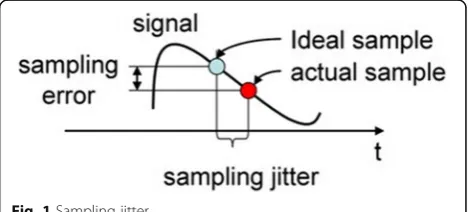
current system and the data instance. The second is that time alignment of multi-sourced data requires that data instances originated from the same node shall have the same interval, or the data instances of different nodes shall be generated at the same time [19]. It can be mea-sured by the jitter size. Figure1shows an example.
Definition 3 (Time-dependent indicator) Assuming that the monitoring area has n nodes, the monitoring time duration is T, and collection interval of all the nodes is Δt. The volatility is defined as the length of time during which the data remains valid:
volatility¼k Δt; ð7Þ
in which, k is a constant which can be chosen for
different values in various situations.
The timely measure of the data of node i in the momenttis defined as currency, that is
currency¼ðtreal–tidealÞ þðtarrive–tidealÞ; ð8Þ where tideal is the ideal sampling time and treal is the
actual sampling time. The system time needed for sink nodes receiving the data recording istarrive.
The time-dependent indicator of data X(i, t) is described as follows:
ftðX ið Þ;t Þ ¼ max 0;1–currency volatility
: ð9Þ
Then, we have the time-dependent indicator of dataset Das follows:
The correctness indicator describes the closeness of the monitored value to the true value. To the data obtained from one sampling of a specific physical quantity (such as temperature), the data is considered to be correct in the case that the data error between the measured value and the real value of the environment is less than a given threshold.
Definition 4 (Correctness indicator) Assuming that the monitoring area has n nodes, the monitoring time duration is T, and all nodes collect data with the same time interval Δt. The data sequence of the node iin the monitoring durationTisXi= [X(i, 1),X(i, 2),…,X(i,T/Δt)].
The observation value can be expressed as val = valreal
+Δ, which is a combination of the real value of the
environment valrealand errorΔ. The correctness of nodei
at timetis defined as follows:
faðvaltÞ ¼ 01;;ΔΔ<>ξξc c
; ð11Þ
whereξcis the error threshold.
The correctness indicator of dataset D is defined as follows:
4.5 Data quality evaluation coefficient
Definition 5 (Data quality evaluation coefficient) Given the dataset Din the time durationT, the data qualityQ is the weighted combination of the data quantity, correctness, completeness, and time-related indicator.
Q¼ ðX
In whichwiis the weight of each indicator.
5 Method
Data management requires not only data quality assess-ment but also high-quality datasets obtained by data clean-ing or other technologies. Quality assessment indicators will affect each other in the data cleaning process. This paper aims at finding the relationship between quality indicators as well as a proper data cleaning strategy. It is noted that the relationship between indicators analyzed in the following is considered in the data cleaning process if it is not specialized.
5.1 Relationship between data volume indicator and others
Theorem 1The data volume indicator and completeness indicator are not completely correlated.
Proof Given the time durationT in the same location, the sampling frequency Δt, data sequences collected by unreliable nodes isXi= [X(i, 1),X(i, 2),…,X(i,T/Δt)], and
by the reliable nodes is Xi′= [X′(i, 1),X′(i, 2),…,X′(i,T/
Δt)]. The data sizes are denoted as vi and vi′,
respectively, in whichvi′>vi.
For sequence Xi, the probability is ploss in case that
instanceX(i,t) is independently lost. Therefore, the data volume, cvt, satisfies the binomial distribution by
following the completeness constraint. For data sequenceXi′, the probability isplossandcvt′satisfies the
binomial distribution too. According to the Formula (6), the variation of the completeness indicator is as follows:
Δqc¼
in which cvt and cvt′ satisfy the binomial distribution
respectively.
So, we havep(Δqc≥0)∈(0,1). In this way,qv~≺qc■.
Theorem 2 The data volume indicator and time cor-relation indicator are not completely correlated.
Proof Given the time durationT, let vi be the size of
data sequence Xi collected by unreliable nodes, and vi′
be the size of data sequence Xi′ collected by reliable
nodes. The probability isptimein the case that data has
independent jitter. The data instance satisfies the normal distribution during the network transmission. According to Formula (10), variation of the time correlation indica-tor is described asΔqt=qt−qt′:
in which qt and qt′ are independent to each other and
satisfy the binomial distribution respectively.
So, we have p(Δqt≥0) ∈ (0,1). In conclusion, there is
not a complete correlation between data volume indica-tor and correctness indicaindica-tor, which can be described as qv≺~qt ■.
Theorem 3 The data volume indicator and the cor-rectness indicator are not completely correlated.
Proof Similar to the proof process of Theorem 1, the probability isperrorfor the situation that data instance is
independently wrong. According to Formula (12), cor-rectness indicators qa and qa′ are independent of each
other and respectively satisfy the binomial distribution. We have Δqa=qa′ −qa in whichp(Δqa≥0) ∈(0,1). So,
we haveqv≺~qa ■.
5.2 Relationship between completeness indicator and others
Theorem 4 There is a positive correlation between the completeness indicator and data volume indicator.
Proof In the time duration T, the data sequence of node i is Xi= [X(i, 1),X(i, 2),…,X(i,T/Δt)]. The missed
data is shown below:
X ið Þ ¼;t null orxj¼null; ð16Þ
However, the data is not lost after data repair. Accord-ing to Definition 1, we have
Δqv¼
Theorem 5 There is no correlation between the com-pleteness indicator and the time-related indicator after repairing the missing data of the dataset assuming that only the collected data is calculated by the time-related indicator.
Proof In the time duration T, the data sequence of nodeiisXi= [X(i, 1),X(i, 2),…,X(i,T/Δt)]. When there is
a data loss, we have
X ið Þ ¼;t null orxi¼null;X ið Þ;t
¼fx1;x2;…;xkg: ð18Þ
After data cleaning by fixing these missed data, these values are no longer empty, and thus the data volume will increase fromcvttocvt′.
However, this increment is independent to the time because it is carried out at the sink node.
According to Formula (10),Δqt= 0. So we haveqc⊀qt■. Theorem 6There is no complete correlation between the time correlation indicator and completeness indicator.
Proof In the time duration T, the data sequence of node iis Xi= [X(i, 1),X(i, 2),…,X(i,T/Δt)]. The data loss
is represented as valt=null, where valt∈ Xi.
Complete-ness cleaning will add the lost data into the sequence, and thus the data volume increases fromcvitocvi′, and
we have:
Δcvi¼cv
0
i−cvi:
Suppose the correctness of the repaired data is judged as probabilitypr, that is
p fð aðvaltÞ ¼1Þ ¼pr;valt^IΔcvt
According to Formula (12), the probability isp(Δqt≥0) ∈(0,1) withΔqt≥0:
5.3 Relationship between time correlation indicator and others
Theorem 7There is no correlation between time correl-ation indicator and data volume indicator.
Proof The timeliness measurement is calculated by Formula (8), and we can see that the currency ofX(i,t)
decreases after data cleaning because the jitter is elimi-nated. At the same time, the cleaning does not increase the sampling records, which means that X(i, t) is not changed. According to Definition 1, we haveΔqv= 0. So,
we haveqt⊀qv■.
Theorem 8 The time correlation indicator and completeness indicator are irrelevant.
Proof According to the definition of timeliness meas-urement, currency decreases because the jitter is elimi-nated after the data related cleaning process, while
ƒc(X(i, t)) remains unchanged for X(i, t). According to
Definition 2, the effective data volume cvt=∑ƒc(X(i, t))
remains unchanged. According to Formula (14), we have Δqc= 0. So, we haveqt⊀qc■.
Theorem 9In the case that the physical signal changes continuous and smoothly, there is a positive correlation between time-related indicator and correction indicator after eliminating jitter in the collected dataset.
Proof As shown in Fig. 1, the sampling time is treal=
tideal+Δt, while the observation value is val = valreal+Δ,
whereΔis the error caused by the jitterΔt.
Considering the general situation, the physical signals observed by the nodes change continuously and smoothly in a long period of time, and the sampling fre-quency of the nodes is far less than the frefre-quency of sig-nal changes. When the sampling delay Δtdecreases, we can assume the error Δ decreases too. According to Definition 4, fa(valt) = 1 when Δ<ξc. So, ∑fa(valt)
in-creases for a given data sequence Xi. According to
Formula (12), we haveΔqa> 0. So, we getqt≺qa■.
5.4 Relationship between correctness indicator and others
Theorem 10There is no correlation between the correct-ness indicator and the data volume indicator.
ProofThe observed value can be described as val=
val-real+Δ, in which Δ is the error. In the case that Δ>ξ,
the value is considered as abnormal and the correctness data cleaning will eliminate the data error, and accord-ingly, we have fa(valt) = 1. At the same time, the
com-pleteness metric for dataset Dat time t is not changed according to Definition 2, which means Δqv= 0. So, we
haveqa⊀qv■.
Theorem 11 There is no correlation between the cor-rectness indicator and the completeness indicator.
Theorem 12 There is no correlation between the cor-rectness indicator and the time correlation indicator.
Proof The proof process is similar to that in Theorem 10■.
5.5 Analysis of sequential cleaning strategies
demonstrate the positive/incomplete correlations be-tween these data quality indicators separately.
Assuming that many data errors, such as jitter, data loss, and data exception, occur in the collected datasetD. The existence of these errors leads to lower metrics for these data indicators, i.e.,qc,qt, andqa. There are several
combi-nations for the data cleaning strategies in which the clean-ing process is carried out with different orders:
(1)Completeness, time-related, and correction;
(2)Completeness, correction, and time-related; (3)Time-related, completeness, and correction; (4)Time-related, correction, and completeness; (5)Correction, completeness, and time-related; (6)Correction, time-related, and completeness.
According to the relationship analysis in the previous section, completeness cleaning cannot guarantee the data correctness, and thus abnormal data might still exist if it is placed at the end of the cleaning order. It means that
Fig. 2The positive correlation between data quality indicators
(4), (5), and (6) are not suitable for the WSNs. In order (3), the performance of the time-related cleaning algo-rithm cannot be guaranteed, especially in the case that data loss is serious in the original dataset. In order (2), it is helpful to reduce the abnormal data by eliminating the jitter. However, if there is a peak among two adjacent col-lections, Theorem 9 does not stand, which means possible poor performance after the cleaning process.
On the other hand, if we adopt the order (1), the com-pleteness data cleaning is firstly carried out, which will repair the lost data and is helpful to guarantee the per-formance of the secondary time-related data cleaning. The final correctness cleaning will eliminate the abnor-mal data due to the previous two steps, and the final metrics for these three indicators will increase accord-ingly. In this way, we can see that order (1) is the best compared with other strategies.
5.6 Data cleaning strategy
According to the analysis of the final cleaning effect of different cleaning sequences in the previous section, it is considered that the data cleaning strategy by order (1) is the best one. Therefore, in this paper, we propose the following data cleaning strategy to avoid redundant cleaning operation and reducing the cleaning expenses as well as ensuring the data cleaning effect.
Step 1 Calculate the volume indicator of datasetD. Step 2 If the volume indicator is larger than a given
threshold, then
Step 3 Clean the dataset by completeness indicator; Step 4 Clean the dataset by time-related indicator; Step 5 Clean the dataset by correctness indicator; Step 6 End.
Steps 1 and 2 are used to determine if the cleaning process is necessary or not. The volume indicator de-scribes the size of the collected data. If the size is very small, it might show that the network is not in the proper mode because enough data cannot be gathered by the system. The reliability for these data is very low in this case. Although data cleaning is helpful to repair the lost data, it is considered useless since the reliability is less than the threshold. Steps 3 to 5 will carry out the cleaning process via completeness, time-related, and cor-rectness indicators, as mentioned in the previous section.
6 Simulation
The simulation is carried out based on the dataset of inter indoor laboratory project with MATLAB as the simulation tool. The project includes 54 Mica2Dot sensor nodes in Intel Berkeley Research Lab. The temperature, humidity, and light data of the environment are collected every 30 s
by the nodes. Data are gathered through the TinyDB intra-net query processing system [20]. In this paper, data clean-ing is carried out with the abnormal data detection and correction technology based on small waves, the elimin-ation sampling shaking technique based on linear interpolation, and the missing data patch technology based on KNN. We firstly verify Theorem 1 to Theorem 12 by different groups of simulations. Then, we carry out the cleaning strategy with temperature dataset and com-pare the final result with the practical values. Finally, the performance of the proposed data cleaning strategy is demonstrated.
6.1 Correlation simulation
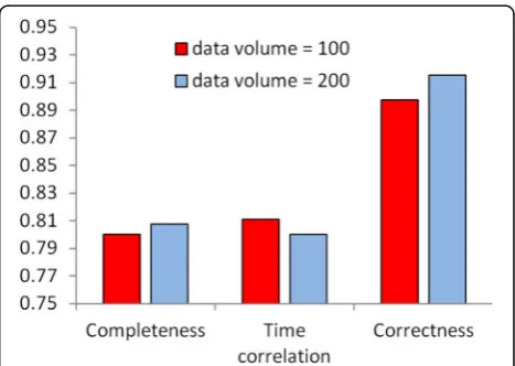
This group of simulations demonstrates the relationship between the volume and other indicators. Data loss, jitter, error, and other mistakes in the dataset are independent and consistent with binomial distribution. In this paper, two data volumes are gathered at time Δt and 2Δt, and the metrics in other indicators of these two datasets are calculated respectively. The results are as follows.
As we can see in Fig.4, in the case that the data volume of each node changes from 100 to 200, the metric of the time-dependent indicator decreases, the dataset complete-ness increases slightly, and the correctcomplete-ness indicator increases. It shows that the impact of the data volume on the other three indicators is not certain. As the data volume increases, the other three indicators may increase or de-crease simultaneously. Thus, Theorems 1 to 3 are verified.
The next group of simulation deals with the relation-ship between completeness and other indicators. Given one dataset, we carry out the completeness cleaning two times which will increase the completeness indicators. Then, we can observe the difference between the other three indicators.
As we can see in Fig.5, in the case that the complete-ness increases, the time-dependent indicator is almost
unchanged, while the correctness indicator will increase or decrease. It can be seen that the variation of the time-dependent and correctness indicator is uncertain while carrying out the completeness cleaning. At the same time, the mending of missing data will repair partial lost data. According to Definition 1, the data volume of nodes will increase. Thus, Theorems 4 to 6 are verified.
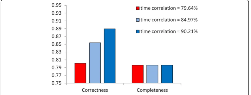
The following group of simulations deals with the rela-tionship between time-dependent and other indicators. Similar to the above experiment, the sample jitter is eliminated twice on the same dataset in order to guaran-tee that the time-dependent indicator of the dataset gradually increases. Then, we can observe the difference between the other three indicators.
As shown in Fig.6, the cleaning process by eliminating the sample jitter will enhance the time-dependent as well as the correctness indicator, while the completeness indica-tor remains unchanged. Thus, Theorems 7 to 9 are verified.
The following group deals with the relationship be-tween correctness and other indicators. Twice, data cleaning operation for the abnormal data are carried out sequentially, and thus the correctness will increase ac-cordingly. Then, we can observe the difference between the other three indicators.
As we can see in Fig.7, the cleaning process by elimin-ating the abnormal data will enhance the correctness, but the time-related and completeness indicators remain unchanged. Thus, Theorems 7 to 9 are verified.
6.2 Data cleaning simulation
In order to verify the performance of the proposed data cleaning strategy, we adopt two different sequential cleaning strategies under the same cleaning cost. The data before cleaning and the cleaned data are respect-ively compared with the true values of the environment so that the difference between them can be observed
Fig. 5The effect of completeness on other indicators
intuitively. The cleaning costs of the two cleaning strat-egies are the same and abnormal data detection and cor-rection, missing data mending, and linear interpolation cleaning operation for eliminating sample jitter are re-spectively performed. Due to the fact that the practical value of the environment in the experiment is not avail-able, we use the average of 54 nodes as the practical value of the environment.
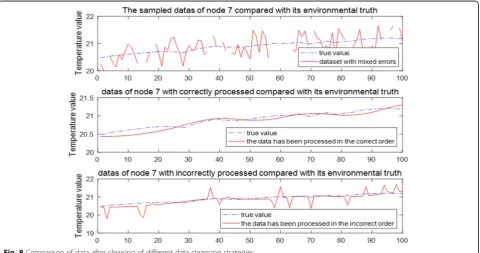
As we can see from the first value in Fig.8, there are many errors, such as data loss, gross error, and sample jitter in dataset D of node 7. The quality metrics Q is 65.34%. When D is cleaned with the proposed data cleaning strategy, the final datasetD′is more similar to
the practical value (the second one in Fig. 2). The new quality metrics Qis 89.43%. We also carry out the data cleaning strategy with order (4) in Section 4.5, and com-pare the performance with the practical value (the last one in Fig. 8). It can be seen that the proposed data cleaning strategy performs a better cleaning effect on datasetD.
7 Conclusions
Reasonable data cleansing strategies which can effect-ively improve data quality and remove extra cleaning overhead caused by repeated cleansing are very import-ant to data management in wireless sensor networks. In
Fig. 7The effect of correctness on other indicators
this paper, we introduced four data quality indicators, namely, data volume, completeness, time-dependence, and correctness. Theoretic analysis with respect to their relationships was provided. We analyzed the cleaning ef-fect of different order of cleaning strategy and proposed a data cleaning strategy that is suitable for the wireless sensor networks. Additionally, detailed simulations were carried out to demonstrate the correctness and perform-ance of the suggested data cleaning strategy. The pro-posed data cleaning strategy has a significant effect on improving data availability.
Acknowledgements None.
Funding
This work is supported by the National Science Foundation of China under Grant No. 61370210, the Program for New Century Excellent Talents in Fujian Province of China under Grant No. SX2015-01, and the Fujian Province Key Laboratory of Network Computing and Intelligent Information Processing Project under Grant No. 2009J1007.
Availability of data and materials None.
Authors’contributions
HC proposed the framework of the data cleaning strategy. Moreover, he also participated in the writing of this paper. DF carried out the simulation. XS contributed to the relationship analysis of these indicators, and he wrote the initial version of this paper. CC contributed to the performance analysis. All authors read and approved the final manuscript.
Competing interests
The authors declare that they have no competing interests.
Publisher’s Note
Springer Nature remains neutral with regard to jurisdictional claims in published maps and institutional affiliations.
Received: 2 January 2018 Accepted: 28 February 2018
References
1. C Batini, M Scannapieco,Data quality: concepts, methodologies and techniques(Springer Publishing Company, 2010). https://doi.org/10.1007/3-540-33173-5 10.1109%2FICCSE.2012.88
2. D Ganesan, S Ratnasamy, H Wang, et al., Coping with irregular spatio-temporal sampling in sensor networks. ACM Sigcomm Comput Communication Rev
34(1), 125–130 (2004).https://doi.org/10.1145/972374.972396
3. A Karkouch, H Mousannif, HA Moatassime, et al., Data quality in internet of things: a state-of-the-art survey. J Network Comp App73(57–81) (2016).
https://doi.org/10.1016/j.jnca.2016.08.002
4. S Sicari, C Cappiello, FD Pellegrini, et al., A security-and quality-aware system architecture for Internet of Things. Inf. Syst. Front.18(4), 665–677 (2016).
https://doi.org/10.1007/s10796-014-9538-x
5. A Klein, W Lehner, Representing data quality in sensor data streaming environments. J Data and Inf Qual1(2), 1–28 (2009).https://doi.org/10.1145/ 1577840.1577845
6. F Li, S Nastic, S Dustdar,Data quality observation in pervasive environments, IEEE 15th International Conference on Computational Science and Engineering (CSE), 602–609 (2012).https://doi.org/10.1109/ICCSE.2012.88
7. W Fan, S Ma, N Tang, et al., Interaction between record matching and data repairing. J Data Inf Qual. 4(4), 16 (2014). DOI:https://doi.org/10.1145/2567657
8. XO Ding, HZ Wang, XY Zhang, et al., Research on the relationship of data quality with many kinds of properties. J Software27(7), 1626–1644 (2016).
https://doi.org/10.1007/s10115-011-0474-5
9. O Ghorbel, W Ayedi, H Snoussi, et al., Fast and efficient outlier detection method in wireless sensor networks. IEEE Sensors J.15(6), 3403–3411 (2015).
https://doi.org/10.1109/JSEN.2015.2388498
10. Y Zhuang, L Chen, In-network outlier cleaning for data collection in sensor networks. Int'l VLDB workshop on clean databases, Cleandb (2006). Seoul Korea. DBLP (2006). DOI:https://doi.org/10.1007/s10115-011-0474-5
11. A Hamrani, I Belaidi, E Monteiro, et al., On the factors affecting the accuracy and robustness of smoothed-radial point interpolation method. Adv. Appl. Math. Mech.9(1), 43–72 (2016).https://doi.org/10.4208/aamm.2015.m1115
12. YY Li, LE Parker, Nearest neighbor imputation using spatial–temporal correlations in wireless sensor networks. Inf Fusion15(1), 64–79 (2014).
https://doi.org/10.1016/j.inffus.2012.08.007
13. E Rahm, HD Hong, Data cleaning: problems and current approaches. IEEE Data Eng Bull23(23), 3–13 (2000).https://doi.org/10.1007/978-0-387-39940-9
14. S Sathe, TG Papaioannou, H Jeung, et al.,A survey of model-based sensor data acquisition and management. Managing and mining sensor data
(Springer, US, 2013), pp. 9–50.https://doi.org/10.1007/978-1-4614-6309-2_2
15. CC Aggarwal,Managing and mining sensor data, Springer US (2013).https:// doi.org/10.1007/978-1-4614-6309-2
16. RY Wang, DM Strong, Beyond accuracy: what data quality means to data consumers. J. Manag. Inf. Syst.12(4), 5–33 (1995).https://doi.org/10.1080/ 07421222.1996.11518099
17. L Jiang, A Borgida, J Mylopoulos,Towards a compositional semantic account of data quality attributes. International Conference on Conceptual Modeling ER 2008(2008), pp. 55–68.https://doi.org/10.1007/978-3-540-87877-3_6
18. C Zhang, X Zhou, C Gao, C Wang, On improving the precision of localization with gross error removal. IEEE ICDCS (2008). 144–149. DOI:
https://doi.org/10.1109/ICDCSWorkshops.2008.44
19. M Suzuki, S Saruwatari, N Kurata, et al., A quantitative error analysis of synchronized sampling on wireless sensor networks for earthquake monitoring. ACM Conference Embedded Network Sens Syst, 417–418 (2008).https://doi.org/10.1145/1460412.1460481