Iberia Azores Gravity Model (IAGRM) using multi source gravity data

(1)

Iberia-Azores Gravity Model (IAGRM) using multi-source gravity data

J. Catalao

LATTEX, University of Lisbon, Faculty of Sciences, Campo Grande, 1749-016 Lisbon, Portugal

(Received April 20, 2005; Revised September 15, 2005; Accepted September 27, 2005; Online published March 10, 2006)

A consistent high precision and high resolution gravity model in the north-east Atlantic off Iberia peninsula using multi-source gravity data, ship-borne and satellite derived gravity anomalies, is presented. A solution strategy based on least squares optimal interpolation was used to assimilate into a coherent gravity model, gravity data with different spectral and spatial resolutions. Satellite derived gravity anomalies from KMS02 model, with an error covariance of 25 mGal2, and marine data carefully edited and validated by bias cross-over error adjustment, were used in this study. The observation error variance was determined from ship-borne track adjustment and assigned an independent value for each track determined from error variance propagation. Unbiased ship-borne gravity observations were assimilated into the satellite derived gravity KMS02 model by the least squares optimal interpolation algorithm (OI) with bias removed by applying a regional bias to all ship tracks (OI-b) and alternatively by constraining all ship tracks to KMS02 using bias and tilt (OI-t). External error of the model was determined by comparing with recent surveys and it was verified that OI-t approach improved the final gravity model to an accuracy of about 3 mGal. The effect of different merging approaches on geoid solution was also evaluated and it was verified that the merging process can contribute to improve the geoid accuracy up to 4 cm with the OI-t approach.

Key words:Gravity, merging techniques, Iberia-Azores, optimal interpolation.

1. Introduction

New methods and tools to support gravity data collection were developed worldwide in the last ten years (Childers

et al., 2001; Forsberg and Brozena, 1992; Forsberget al., 1997; Schwarz and Li, 1996; Kearsleyet al., 1998). Grav-ity data from marine or terrestrial surveys, airborne grav-ity, satellite altimeter derived gravity and space gravity mis-sions are widespread techniques that are able to supply large amounts of gravity data with unprecedented resolution and precision. However, this new data from satellite missions is bandwidth limited and marine gravity data or airborne gravity data could be used to recover the high frequencies of the gravity spectrum (Kernet al., 2003). Moreover, its usefulness will be limited in costal areas where altimeter data suffers for large errors that can contaminate the derived gravity anomalies (Denget al., 2002; Rodriguez-Velascoet al., 2002). By other hand, marine gravity anomalies are ir-regularly distributed on sea, with sparse tracks crossing the sea, but with a clear densiﬁcation in coastal areas and near continental margin. Clearly, both data sets are complemen-tary in geographic data distribution and on geographic data quality, demanding we pursue methods to assimilate both into a better gravity data model that incorporates high fre-quency information and precision from marine gravity data with the high spatial coverage and (in some areas) less pre-cise data from the satellite derived gravity anomalies. The great challenge of the integration of multi-source gravity

Copyright cThe Society of Geomagnetism and Earth, Planetary and Space Sci-ences (SGEPSS); The Seismological Society of Japan; The Volcanological Society of Japan; The Geodetic Society of Japan; The Japanese Society for Planetary Sci-ences; TERRAPUB.

data is to derive a gravity model that incorporates the most accurate data with the best spatial resolution.

There are basically two main approaches for the combi-nation of multi-source gravity data: one that operates on spatial domain working on the observation level and other that operates on the frequency domain combining data spec-tra. A solution for the combination of more than two data sources in the frequency domain was proposed by Kernet al.(2003). In this paper, a strategy is presented for the com-bination of heterogeneous data using spectral weights. This method relies on Least Squares spectral combination and requires the determination of spectral weights that are as-sumed to be error degree variances of local anomaly data and from satellite data. The drawback of this method is the required knowledge of the local data degree variances that are not known and must be estimated. Besides that, this method requires a regular distribution of observation data that it is not veriﬁed for shipborne surveys or even for air-borne surveys.

On spatial domain, an operational strategy for combin-ing different quality levels of gravity anomalies and dif-ferent data resolution was already suggested by Strykowski and Forsberg (1998). The proposed method was an n-step process that maps less quality anomalies into better preci-sion gravity anomalies data set, through the use of a resid-ual surface computed from the difference between the ﬁrst and the second model. In this method, a global precision is attributed for each data set discarding the possibility of local or regional variations in the precision given by dif-ferent tracks surveyed in difdif-ferent epochs. Another similar, but more elaborated method, was proposed and analyzed by Olensen et al.(2002) in which satellite altimetric data

(2)

278 J. CATALAO: IBERIA-AZORES GRAVITY MODEL USING MULTI-SOURCE GRAVITY DATA

and marine gravity data are mixed using least squares col-location. These authors present two different merging tech-niques, both based on collocation, that combines airborne gravity observations with either geoid observations derived from satellite altimetry or gravity derived from satellite al-timetry. They veriﬁed that collocation approach, based on the combination of geoid satellite altimetry, gives slightly better results than the global mixing approach with only gravity data (satellite derived and airborne data). Although least squares collocation uses randomly distributed data, it requires intensive computation time and the proposed method requires the processing of satellite altimetric obser-vations.

In this paper, we present an alternative method based on least squares Optimal Interpolation (Moritz, 1980; Boutier and Courtier, 2002) that combines two or more gravity data sets with their associated error variances into another grav-ity data set that is statistically optimal. This method is eval-uated and its performance is compared with aforementioned methods (least squares collocation and drape technique). The study is carried out on the North-Atlantic Ocean be-tween Iberian Peninsula and the Azores archipelago where satellite derived gravity anomalies from KMS02 (Andersen and Knudsen, 1998) and marine gravity data exists with dif-ferent spectral and spatial resolutions, and involves difdif-ferent types of morphological structures from coastal areas, deep ocean to inter-islands areas. To access the accuracy of the resulting gravity model, airborne gravity data, not used in the merging process and recent shipborne gravity data was used. Also the geoid for this area was computed and its accuracy evaluated on sea by comparison with 10 year of Topex data and on land with GPS/levelling data.

2. Mathematical Background

Considering the real value of the gravity anomaly (not known) as gr(φ, λ) and the background model as gb(φ, λ), representing theaprioriknowledge of the grav-ity anomaly ﬁeld before the analysis is carried out, the anal-ysis problem is to ﬁnd a correctionδg(φ, λ)that:

ga(φ, λ)=gb(φ, λ)+δg(φ, λ) (1) is much closer to the real gravity anomaly ﬁeldgr(φ, λ)

than the background model (Boutier and Courtier, 2002). The correction gridδg(φ, λ)is determined by the obser-vation data. The obserobser-vation data is irregularly distributed and is assembled into an observation vector with N data val-ues. The best way to compare the observation data with the background model is through the use of a mapping function

f(φ, λ)which calculates the model equivalent of the ob-servation, and is called observation operator. In the general case, the observation vector can be a composite of grav-ity anomalies or any other gravgrav-ity ﬁeld related observation, like vertical deﬂections or sea surface height or geoid un-dulation. In this case, the observation operator will map the observation space into the background model using the fun-damental equation of the physical geodesy (Heiskanen and Moritz, 1967) or any other related function. Assuming that errors are unbiased, the optimal least-squares estimation for the discrepancies is (Moritz, 1980):

ga =gb+K(gobs− f((φ, λ)) (2) and

K =B FT(F B FT +D)−1 (3)

where K is the weight matrix and the other error covari-ances areBfor the background model andDfor the obser-vation, andFis transformation matrix between the signals. This is the solution for the global or regional analysis problem which requires inverting a matrix with a large di-mension, equal to the number of observations (N), which in earth sciences can be thousands or millions. The Optimal Interpolation (OI) analysis is a computational simpliﬁcation of the matrix inversion in Eq. (3). In OI the weight matrix is simpliﬁed by assuming that only the closest observations determine the incrementδg(φ, λ). OI implementation

re-quires the knowledge of the background error covarianceB

and the observation error covariance D. The matrix D is supposing a diagonal matrix with the estimated observation variance. This estimated precision is the result of a marine (or terrestrial) gravity network adjustment or can be empiri-cally based on the acquisition date, equipment and all other relevant information. The covarianceBportraits the corre-lation model that “correlates” the background model with the observation data. This matrix is defined locally for each local variable through an empirical autocorrelation function (Barzaghi and Sansò, 1983; Forsberg, 1984; Moritz, 1980) and must be positive definite.

This solution assumes that the discrepancies are unbi-ased, which means that the difference between the given set of observations and the background model is null (or close to) in the considered geographic domain. In gravity field modelling this hypothesis is very difficult to be veri-fied. Shipborne gravity measurements are relative to some known base station and, therefore, any incorrect tie-in to that station may lead to a constant offset in all gravity data of that cruise. Assuming that background model is unbi-ased, the detected bias on the observations is removed and the above equations applied to the unbiased observations. It is important to detect and control the biases by analyz-ing previously the background model and the observations contrasting them with other source of data and/or related gravity field data. In this paper we have also analysed this key aspect by considering two different bias removal ap-proaches.

3. Gravity Data

3.1 Surveyed Gravity anomalies

(3)

Fig. 1. Marine gravity data collected from BGI, NGDC and AGMASCO project in North-East Atlantic between Iberian Peninsula and Azores archipelago.

mean length of 199 km and a maximum length of 4264 km. All data were transferred to IGSN71 system and the anoma-lies converted to GRS80. Geographical distribution of ity data is depicted in Fig. 1. In our study area, marine grav-ity measurements obtained before the 80’s represents more than 66% of the total of available gravity observations.

Marine gravity data was validated and adjusted with spe-ciﬁc software, written for this purpose, Catalao and Sevilla (2004). Spatial intersections between tracks (cross-over points) were determined (3992 intersections) and the ex-ternal Crossover Errors (COE) were computed for each in-tersection. The external COE had a standard deviation of 10.81 mGal and a minimum and maximum value of−94.87 mGal and 103.47 mGal, respectively. The amplitude of the COE is almost half of the gravity signal in this area, mean-ing that there are large discrepancies in the gravity observa-tions belonging to different missions.

Track bias was determined through a global adjustment of the external COE and different weights to each obser-vation equation were given. The minimum constraint ad-justment was adopted with a one step global adad-justment constraining to a zero bias the PDIC/C/MAR, surveyed in 1997. A standard deviation was attributed for each cruise or leg based on its surveying date in which for the most re-cent tracks (after 1980) a 2.5 mGal standard deviation was considered, for the tracks between 1970 and 1980 a value of 7.5 mGal was considered and for tracks before that date (1970) a value of 12.5 mGals was considered for standard deviation.

After the adjustment, the standard deviation of the cross over errors reduces to 3.0 mGal, with a minimum and max-imum reduced to−28.5 and 28.7 mGal, respectively. The adjustment solution (bias) was applied to each track and the associated individual (for each track) estimated standard deviation was assigned to each observation belonging to a track. The resulting ﬁle has 157,758 gravity anomaly obser-vations with an associated standard deviation that does not

reﬂect its own estimated precision but the overall quality of the track it belongs to.

3.2 Satellite derived gravity anomalies

There are several public domain altimetric derived grav-ity anomalies data sets with a global coverage. These mod-els, in grid format, were computed directly from sea surface heights, KMS02 (Andersenet al., 1999), or through deﬂec-tions of the vertical (Sandwell and Smith, 1997). KMS02 is the latest of a series of satellite derived gravity anomalies data sets supplied by Kort-og MatrikelStryrelsen and can be free downloaded from ftp.kms.dk. Numerous comparisons between marine observations and satellite altimetry derived gravity anomalies data sets have been presented (Andersen and Knudsen, 1998, Sandwell and Smith, 1997). The re-ported precision ranges from 3 mGal to 14 mGal as a func-tion of the geographic locafunc-tion. In the North-Atlantic the reported precision for Sandwell and Smith (1997) model is 7.6 mGal and for KMS model is 5.8 mGal (Andersen and Knudsen, 1998). KMS02 shows the best agreement with ship-borne gravity data and because of this we have adopted this model (KMS02) as our background model.

(4)

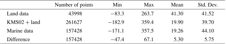
Table 1. Differences between KMS02 gravity and marine gravity data (in mGal).

Number of points Min Max Mean Std. Dev.

Land data 43998 −83.3 263.7 41.30 41.52

KMS02+land 261627 −182.9 359.4 19.90 39.70

Marine data 157428 −171.1 357.5 19.26 44.10

Difference 157428 −47.4 67.1 5.30 5.75

4. Merging by Optimal Interpolation

The basic principle underlying OI algorithm is the exis-tence of a background gravity model that completely covers all geographic domains. This model is the first guess of the gravity field and must be complemented with an associated error covariance model. This requirement is completely accomplished by the altimetric derived gravity anomalies, when complemented with land gravity data. In this circum-stance, shipborne gravity data and its associated covariance error model are the observation set that will contribute to the improvement of the first guess model.

Accordingly with Eq. (2) the discrepancies between the background model and the observation set must be deter-mined in the observation position. The background model is a discrete model, and the observation set is irregularly distributed, this means that they do not coincide, and an interpolation function must be derived to evaluate the back-ground model in the observation position. Least squares prediction was used for this purpose with a correlation dis-tance of 10 km and a covariance error model determined from the background gravity data. The background error covariance matrix is determined with a second a second-order Markov covariance function of the form (Forsberg, 1984):

C(ψ)=C0(1+ψ/φ1)e−ψ/φ1 ₍₄₎

where ψ is the spherical distance, C0 is the background model variance and φ1 is the correlation distance deter-mined from the background model. The discrepancies be-tween the background model and the observations are listed in Table 1. In this Table is shown that both data sets have a similar behaviour with a similar amplitude and standard deviation and almost equal mean value. It is important to notice that in the background model is also included land gravity data that may reflect the difference in the standard deviation. Differences were computed only at marine grav-ity data points and exhibit a mean value of 5.3 mGal and a standard deviation of 5.75 mGal in agreement with the results presented for this area by Andersen and Knudsen (1998). Results of this comparison shows that there is no perfect agreement between observed gravity anomalies and altimeter derived ones, reaching differences of more than 60 mGal. A residual mean value of 5.3 mGal means that one of the data sets is biased and in the worst situation both are bi-ased. Assuming that this residual is the result of shipborne datum inconsistencies and other bias-like effects, bias was removed by adding−5.3 mGal to all marine data, further referenced as OI-b. This approach could not be satisfactory once the gravity field is not homogeneous and local bias is detected. Alternative approach was achieved by fitting

individually ship tracks to the KMS02 model by estimat-ing bias and tilt to each track, further referenced as OI-t. After a careful editing process a crossover adjustment of the tracks was performed subject to the individual ﬁtting to KMS02 model. Individual track discrepancies and a prede-ﬁned threshold level was used to reject bad marine tracks.

The implementation of the optimal interpolation algo-rithm requires the definition of the background error co-variances (Bmatrix) and the covariance error model for the observations (Dmatrix), see Eq. (3). Dmatrix is a diago-nal matrix with the observation covariance error estimated by the marine gravity adjustment. For each observation was assigned a covariance error value equal to the estimated pre-cision of the track it belongs to. The background error co-variance matrix is determined with a second-order Markov covariance function using Eq. (4). In Optimal Interpolation the weight matrix K is simplified by assuming that only the closest observations determine the increment to apply to the background model. In this case, the selection of ob-servations should afford all pertinent obob-servations (with a significant weight) within a given radius around the back-ground model point location. A mix approach based on an equal number of observations and a circular area restriction was adopted. This can be achieved by defining a minimum number of observations and introducing a localization delta functionδ(φ, λ)that acts as a switch in the error value de-termined between the background model and the observa-tion data. Equaobserva-tion (2) assumes the following aspect:

ga=gb+K((gobs− f(φ, λ))∗δ(φ, λ)). (5)

(5)

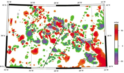
Fig. 2. Mapping function derived by OI applied to the background model. Two tracks (T1 and T2) are also plotted, used for evaluation purposes.

Table 2. Mapping function, original KMS02 gravity ﬁeld, resulting Iberia-Azores Gravity Model (IAGRM), reduced to EGM96 model and residual gravity ﬁeld after the removal of EGM96 and RTM effects (in mGal).

Min Max Mean Std. Dev.

Mapping function −56.8 68.6 0.20 3.97

KMS02 −181.9 359.7 18.18 38.62

IAGRM −178.8 340.6 18.39 38.74

IAGRM-EGM96 −118.4 209.0 0.09 18.58

IAGRM-EGM96-RTM −133.3 147.1 0.28 16.01

Applying this methodology, we solved simultaneously for the extreme spatial irregular distribution of the marine data, for the continuity against neighbour background points and for far distance inﬂuence and inverse distance correlation problem. With a limited selected number observations, the weight matrixK is also limited to the number of points (in this case a maximum of 4×20=80).

Appling the aforementioned methodology, and parame-ters, a correction surface was derived and mapped into the background model. This surface is presented in Fig. 2 lim-ited to the Azores archipelago enhancing the most appealing aspects of the method. The mapping function has a mini-mum value of−56 mGal and a maximum value of 68 mGal between S. Jorge and Pico islands. In this picture the white areas corresponds to areas where the mapping function is between−5 mGal and 5 mGal. The mapping function has extremely irregular behaviour acting on the low wavelength spectrum of the gravity field improving its spectral reso-lution. Statistics for this surface and for the final gravity field in the North-Atlantic are presented in Table 2, with a total of 541581 points. From the results of this table it is verified that there is no gain in the amplitude and the STD is almost the same when comparing KMS02 and IAGRM models. In fact, the background model (KMS02) was only

improved along the ship tracks within a few number of ob-servations (about 13%) and their impact is almost dissolved in the global data set. Even though, in a small area like the one depicted in Fig. 2, the statistic are also very similar but, analysing the differences between these two grids it was verified that the STD of the differences is 3.6 mGal. It is also verified that the residual gravity field, after the removal of long and short wavelengths (EGM96 model and RTM correction), is unbiased and the standard deviation was re-duced to half of the original data. In picture 3 is depicted the final free air gravity anomaly model for the North Atlantic area between Iberia-Azores as a result of the data assimila-tion process.

5. Analysis

The precision and reproducibility of the ﬁnal gravity model was evaluated by comparison with new marine grav-ity data surveyed after 1990, not included in the model, and with other gravity models derived by other methods (Drape technique and Least squares collocation). Besides, the effect of different merging methodologies is evaluated on geoid undulation, comparing with GPS/levelling sites on costal areas and with 10 years of TOPEX data.

(6)

Fig. 3. Gravity ﬁeld model in the North-Atlantic between Iberia and Azores archipelago resulting from the assimilation of marine gravity data into satellite derived gravity by optimal interpolation. GPS/levelling sites are presented as triangles.

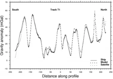
Fig. 4. Comparison of different gravity data types in a shipborne proﬁle (T1) starting in Terceira island running to south-west.

tracks around Azores archipelago, with different estimated error variances. The first one is the most precise track, de-scending from north-east to south-west from Terceira Island (track T1, see Fig. 2) with an estimated precision of 1.5 mGal. The second track is on the south of S. Maria Island and runs also from north to south with an error variance of 15.7 mGal (track T2, see Fig. 2). Background, marine and final models were evaluated in both tracks and a set of pro-files was drawn for track T1 and depicted in Fig. 4. In this figure is seen that there is an almost perfect agreement be-tween satellite and marine gravity data confirming the su-perior quality of the background model (KMS02 satellite

gravity) resolving accurately long wavelengths. In this case, due to the high precision of this marine track (1.5 mGal) the derived gravity model assumes the shipborne data be-haviour increasing signal amplitude and spectral resolution of the satellite data (background model).

(7)

(a)

(b)

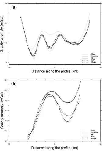
Fig. 5. (a) Short segment of most precise shipborne track (T1). (b) Short segment of less precise ship-borne track (T2). Shipborne data (Ship), back-ground model (satellite), derived model (OI), least squares prediction model (LSP) and drape model (DRAPE) along these tracks are superimposed. Units mGal and km.

final model sticks to the observation data. The opposite ef-fect is seen for track T2, less precise than satellite data, in which the final model sticks to the background model, see Fig. 5(b). The final model tends to assume the behaviour of the most precise data as a compromise between the back-ground and the observation error variance model. This ef-fect was expected and highly desirable allowing the simul-taneous combination of multi-source gravity data into a co-herent gravity model, as long as the error variance are prop-erly assign to each source.

The comparison was also done with other two method-ologies: one step least squares prediction (Tscherning, 1985) and drape technique proposed by Strykowski and Forsberg (1998). These two methods are very similar to

(8)

and T2. In Fig. 5 are also depicted the results of these two methodologies labelled as LSP (Least Squares Prediction) and DRAPE for the drape technique.

In one step least squares prediction both data sets (back-ground model and observations) are treated at the same level and the resulting model is the best least squares esti-mates according to the assumed error variance model. This is particularly evident in the two selected tracks. In T1 track the observation data is much more precise than the back-ground model and as a consequence the final model follows the observation data. In T2 track the background model (satellite data) is more precise than the observation data and the final model follows the background model (the satellite data). We have also analyzed a cross track profile and ver-ified that the observation influence is limited to the along track direction with a rapid decay of the observation value. This is due to the disproportional amount of data used in the LSP process. An isolated track is surrounded by a large amount of data from the background model that envisages the estimation process even if a large precision is assigned to the observation data, limiting its influence to the along track direction.

In drape technique, the background error variance is not explicitly considered and the resulting model exhibits a bet-ter agreement with the observation data, irrespectively its quality. For the most precise track (T1) this corresponds to the expected behaviour of the final model, but for track T2 it is observed that the model follows the observation in a sit-uation that the balance should be to the background model. The drape technique, assumes that the background model is of better quality than the observation data and it does not consider local variations on data quality. The proposed op-timal interpolation scheme reveals a better agreement with the reality than the other two methodologies with a better balance between the weight of the background model and observation data. This is particularly true for irregular and sparse observations as it stands for marine gravity observa-tions surveyed along tracks. For very dense marine gravity data coverage it is believed that these three methods will converge to a very similar solution, but in typical irregular marine data coverage with sparse tracks with known error variance, the optimal interpolation fine-tuned with the local data better reflects the reality.

The reproducibility of the final model was also analyzed numerically computing the misfit between these three dif-ferent final models and the shipborne data. We have consid-ered two situations: residuals of observations with standard deviation less than 5 mGal (observations more precise than the background model) and residuals of observations with standard deviation greater than 5 mGal. In the first case, the three methods return a similar result, ranging the misfit from 1.9 to 2.1 mGal, on the standard deviation, which may be considered as an internal error evaluation. The major dif-ference between these methods relies on the assimilation of less precise observations (withσ > 5 mGal) into the final model. Drape method, with the smaller standard deviation (2.9 mGal), almost follows the observation data, even in this case where the background model is more precise than the observation data. An opposite behaviour is verified with LSP where a value of 6.9 mGal, on the standard deviation,

reveals that ship borne data (observations) were not consid-ered in the assimilation process. The OI algorithm (with 4.8 mGal) reveals a better balanced result with a compro-mise between the standard deviation of the observation data and the background model. These numerical results and the previous graphical representation, of the three methods, demonstrates the skill of the OI method for dealing with multi-source gravity data with different stochastic models assimilating optimally into a coherent gravity data model.

External error assessment was evaluated by comparing with recent marine surveys obtained from the new release of NGDC geophysical data, version 4.1.18. In this recent release, 5 new marine surveys after 1990, that were not in-cluded in the model, were identified (2 in Azores region and 3 close to Iberia). Also, an airborne survey was done in Azores archipelago (Olesen and Forsberg, 1999) in the aim of AGMASCO project, and was used for error evalua-tion. In this campaign Olesen and Forsberg (1999) reported several problems related with a detected bias between air-borne and shipair-borne gravity data which motivate the exclu-sion of this data in our merging process. Some lines showed a bias between 10 to 15 mGal when compared to shipborne gravimetry. Nevertheless, we have considered this data as an external evaluator. Results of these comparisons are pre-sented in Table 3. In this table is seen that the standard devi-ation of the error is almost always smaller for merged mod-els than for the original KMS02 model, with the LSP and OI-t performing better than drape and OI-b methods. There are two situations where it seems there is no improvement (19100041 and 19180010), using OI-t and LSP, which cor-responds to areas where there were no marine data. In this case, OI-b and Drape methods corrupt the original model. Both methods suffers from a bias problem that are not prop-erly handle and are passed through the original model intro-ducing discontinuities in the final gravity model, along the biased track. The improvement is only obtained in areas where marine data is available but is also a function of the method used and also the quality of this new marine grav-ity data. It is seen that OI-t and LSP approaches have the ability to maximize the observation usefulness by propagat-ing its information in space even for randomly distributed data. Survey 67010202 runs through Azores archipelago crossing the inter-island area where altimeter data suffers for several gross errors. Along this track, the standard devi-ation reduces from 12 mGal for KMS02 model to 2.2 mGal and 2.8 mGal revealing an extreme improvement case. The small standard deviation obtained for all methods indicates that the area covered by this track was already improved by other (or others) marine tracks. In general, we are able to say that in costal areas where satellite derived gravity data is less accurate, the inclusion of shipborne gravity data and/or airborne gravity data using OI-t approach will improve the final gravity model to an accuracy of about 3 mGal.

(9)

Table 3. Standard deviation of the comparison between derived models and new surveys performed after 1990 and also with airborne data from Agmasco project (in mGal). Survey name is the survey code in NGDC data set and N the number of observations.

Surv. Name N Kms02 OI-b Drape LSP OI-t

Azores 67010208 3865 4.7 3.2 3.3 3.3 3.1

67010202 2083 12.0 2.2 2.4 2.3 2.8

Iberia 19100041 1446 5.9 6.4 6.7 5.9 6.2

67010183 6456 7.9 2.7 2.9 2.9 3.2

19180010 3391 3.8 4.9 5.1 3.6 3.8

Airborne Agmasco 10005 7.5 6.9 7.2 6.7 6.8

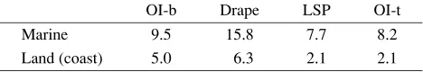
determined using different gravity models derived from abovementioned methodologies. Classical remove-restore methodology was used and the Stokes integral formula was applied. EGM96 geopotential model (Lemoineet al., 1997) to degree and order 360 was used as a reference model and short wavelength topographic effects were computed from the RTM (Residual Terrain Model) (Forsberg and Tschern-ing, 1981) using a medium precision digital terrain model with 500m spatial resolution spanning all area. To evalu-ate the resulting geoid, the absolute geoid undulations were compared with those obtained by 7 GPS/levelling sites on Iberian coast and on Azores islands, see Fig. 3 for site lo-cation. The three Iberian GPS stations are GAIA, CASC and LAGO permanent EUREF stations nearby tide gauges. The other 4 GPS stations, in Azores, TERC, FAIM, GRAC and PDEL (IGS station), are also permanent stations with coordinate repeatability of 2–6 mm for horizontal and ver-tical components (Navarroet al., 2003). On sea, geoid was compared with sea surface heights obtained from 10 years of TOPEX data (Table 4). The comparison determined by GPS/levelling shows that there are significant differences between the four solutions in coastal areas with a maxi-mum of 4 cm between drape technique and OI-t. There is also a significant difference of 3 cm between OI-b and OI-t. These two datasets differ only on the used method for bias removal, revealing that better results are obtained when bias and tilt are removed through individual marine track fitting to the background model. The same conclusion can be drawn from results on sea. In this case, the results obtained from OI-t are almost 2 times better than those ob-tained with drape technique and 1cm when compared with OI-b.

Difference between LSP and OI is more practical than conceptual. In fact, both have the same mathematical for-mulation and stochastic model, the only difference resides on the way data is handled. In LSP, background data and new data are treated at the same level (although with dif-ferent error models) and the system has to manage a large number of data (even millions). In OI approach, new data is treated has a correction to the background model and the system has only to manage a reduced number of observa-tions (the new data). The results of both approaches should be similar as it was veriﬁed.

6. Conclusions

In this study, marine gravity data and satellite derived gravity data from KMS02 were combined to derive a

re-Table 4. Comparison of different geoid solutions computed from dif-ferent merging approaches with 10 year of Topex data (Marine) and GPS/levelling (Land). Presented results are the residual standard devia-tion in cm.

OI-b Drape LSP OI-t

Marine 9.5 15.8 7.7 8.2

Land (coast) 5.0 6.3 2.1 2.1

liable gravity model that will be useful both for geophysical studies and geoid determination. It was shown that com-bined gravity data improves the precision of the derived geoid undulation (both on land and on sea) and the ﬁt to precise shipborne gravity data. This result was particularly obvious in coastal and inter-island areas where satellite de-rived gravity anomalies may contain errors.

It was verified that assimilation with only a regional bias removal (OI-b), introduces discontinuities on the back-ground model delimited by the track envelop (defined by the track influence area). It is likely to be a bias problem that was successfully solved in the OI-t approach where individ-ual tracks are fitted to the background model by a bias and tilt parameter. A similar problem exists in drape technique where the method assumes that the new data is of better quality that the background model which is known not to be true and depends on the satellite derive gravity and on the marine data quality. It was also clear that OI-t and LSP have the same behaviour with a similar performance. Using these methods, the improvement of the final gravity model when compared to the original KMS02 model, is dependent on the geographic area but not on the marine data quality used in the model. It means that there is no model degra-dation and the improvement can reach 10 mGal in rms at inter-island areas.

(10)

op-286 J. CATALAO: IBERIA-AZORES GRAVITY MODEL USING MULTI-SOURCE GRAVITY DATA

timally into a coherent gravity data model with a consider-able recover of the high frequency spectrum of the gravity ﬁeld with a low computational coast when compared with least squares prediction.

Acknowledgments. We are grateful to Eng. Helena Koll from Instituto Geográfico Português for supplying land gravity data on Portugal mainland and we also thank to Dra. Lu´ısa Bastos for the airborne gravity data. The figures have been produced using the GMT software (Wessel and Smith, 1991). This work was funded by FCT (Portuguese Foundation for Sciences and Technology) through KARMA project (POCTI/CTE-GIN/57530/2004).

References

Andersen, O. B. and P. Knudsen, Global marine gravity ﬁeld from ERS-1 and Geosat geodetic mission altimetry,J. Geophys. Res.,103(C4), 8129–8137, 1998.

Andersen, O. B., P. Knudsen, S. Kenyon, and R. Trimmer, Recent improve-ment in the KMS global marine gravity ﬁeld,Bollettino Geoﬁsica Teor-ica ed ApplTeor-icata,40, 369–377, 1999.

Barzaghi, R. and F. Sans`o, Sulla stima empirica della funzione di covari-anza,Bollettino di Geodesia e Scienze Afﬁni,XLII(4), 389–415, 1983. Boutier, F. and P. Courtier, Data assimilation concepts and methods,

Mete-orological Training Course Lecture Series, ECMWF, 2002.

Catalao, J. and M. J. Sevilla, Inner and minimum constraint adjustment of marine gravity data,Computer and Geosciences,30(9–10), 949–957, DOI: 10.1016/j.cageo.2004.06.004, 2004.

Childers, V. A., D. C. McAdoo, J. M. Brozena, and S. L. Laxon, New gravity data in the artic Ocean: Comparison of airborne and ERS gravity,

J. Geophys. Res.,106, 8871–8886, 2001.

Deng, X., W. E. Featherstone, C. Hwang, and P. A. M. Berry, Estima-tion of contaminaEstima-tion of ERS-2 and Poseidon satellite radar altimetry close to the coasts of Australia,Marine Geodesy,25, 249–271, DOI: 10.1080/01490410290051572, 2002.

Fernandes, M. J., A. Gidskehaug, D. Solheim, M. Mork, P. Jaccard, and J. Catalao, Gravimetric and Hydrographic campaign in Azores, in Pro-ceedings of the I Luso-Spanish Assembly in Geodesy and Geophysics, Almeria, Spain, 9–13 Feb., University of Almeria, p. 113, 1998. Forsberg, R., Local covariance functions and density distributions, Dept.

of Geodetic Science and Surveying, Rep. No. 356, The Ohio State University, Columbus, Ohio, 1984.

Forsberg, R. and J. M. Brozena, The Greenland airborne gravity project— comparison of airborne and terrestrial gravity data, inBGI, Bulletin D’Information No. 71, Workshop on marine gravity data validation, Toulouse, Oct. 27–28, 55–58, 1992.

Forsberg, R. and C. C. Tscherning, The use of height data in gravity ﬁeld approximation by collocation,J. Geophys. Res.,86(B9), Sept. 10, 7843– 7854, 1981.

Forsberg, R., K. Hehl, L. Bastos, A. Giskehaug, and U. Meyer, Devel-opment of an airborne geoid mapping system for coastal oceanography (AGMASCO), inProceedings of the International Symposium on Grav-ity, Geoid and Marine Geodesy, GRAGEOMAR, edited by J. Segawa, H. Fujimoto, and S. Okubo, The University of Tokyo, Tokyo, Sept. 30–Oct.

5, 1996, Springer-Verlag, pp. 163–170, 1997.

Heiskanen, W. A. and H. Moritz,Physical Geodesy, W. H. Freeman and Company, San Francisco, 1967.

Kearsley, A. H. W., R. Forsberg, A. Olesen, L. Bastos, K. Hehl, U. Meyer, and A. Gidskehaug, Airborne gravimetry used in precise geoid compu-tations by ring integration,Journal of Geodesy,72, 600–605, 1998. Kern, M., P. Schwarz, and N. Sneeuw, A study on the combination of

satellite, airborne, and terrestrial gravity data,Journal of Geodesy,77, 217–225, DOI 10.1007/s00190-003-0313-x, 2003.

Lemoine, F. G., D. E. Smith, L. Kunz, R. Smith, E. C. Pavlis, N. K. Pavlis, S. M. Klosko, D. S. Chinn, M. H. Torrence, R. G. Williamson, C. M. Cox, K. E. Rachlin, Y. M. Wang, S. C. Kenyon, R. Salman, R. Trimmer, R. H. Rapp, and R. S. Nerem, The development of the NASA GSFC and NIMA Joint Geopotential Model, inProceedings of the International Symposium on Gravity, Geoid and Marine Geodesy, GRAGEOMAR, edited by J. Segawa, H. Fujimoto, and S. Okubo, The University of Tokyo, Tokyo, Sept. 30–Oct. 5, Springer-Verlag, pp. 461–469, 1997. Moritz, H.,Advanced Physical Geodesy, 500 pp., H. Wichmann Verlag,

Karlsruhe, 1980.

Navarro, A., J. Catalao, J. M. Miranda, and R. M. S. Fernandes, Estimation of the Terceira island (Azores) main strain rates from GPS data,Earth Planets Space,55(10), 637–642, 2003.

Olesen, A. V. and R. Forsberg, Azores airborne gravity processing, Per-sonal communication, Copenhagen, March 1999.

Olesen, A. V., O. B. Andersen, and C. C. Tscherning, Merging airborne gravity and gravity derived from satellite altimetry: test cases along the coast of Greenland,Studia Geophys. Geod.,46, 387–394, 2002. Rodriguez-Velasco, G., M. J. Sevilla, and C. Toro, Dependence of mean

sea surface from altimeter data on the reference model used,Marine Geodesy,25, 289–312, DOI:10.1080/01490410290051590, 2002. Sandwell, D. and W. H. F. Smith, Marine gravity anomaly from Geosat

and ERS1 satellite altimetry,J. Geophys. Res.,102(B5), 10039–10054, 1997.

Schwarz, K. P. and Y. Li, What can airborne gravity contribute to geoid determination?,J. Geophys. Res.,101(B8), 17873–17881, 1996. Strykowski, G. and R. Forsberg, Operational Merging of Satellite,

Air-borne and Surface Gravity Data by Draping Techniques, inGeodesy on the Move—gravity, geoid, geodynamics and Antarctica, Proceedings IAG scientiﬁc assembly, Rio de Janeiro, Sept 3–9 1997, Forsberg, Feis-sel and Dietrich (eds.), IAG symposia 119, pp. 243–248, Springer Ver-lag, Berlin, 1998.

Timmen, L., L. Bastos, R. Forsberg, A. Gidskehaug, and U. Meyer, Airborne Gravity Field Surveying for Oceanography, Geology and Geodesy—Experiences from AGMASCO, inIAG Symposia, Volume 121, Springer Verlag, 2002.

Tscherning, C. C., Local approximation of the gravity potential by least squares collocation, inProceedings of the International Summer School on Local Gravity Field Approximation, edited by K. P. Schwarz, Beijing, China, Aug. 21–Sept. 4, 1984, Pub. 60003, Univ. of Calgary, Calgary, Canada, pp. 277–362, 1985.

Wessel, P. and W. Smith, Free software helps map and display data,Eos Trans. AGU,72, 441, 1991.