R E S E A R C H
Open Access
A second-order Fourier pseudospectral
method for the generalized regularized long
wave equation
Xiaorong Kang
1, Kelong Cheng
1and Chunxiang Guo
2**Correspondence: [email protected] 2School of Business, Sichuan University, Chengdu, 610064, P.R. China
Full list of author information is available at the end of the article
Abstract
We present a second-order in time linearized semi-implicit Fourier pseudospectral scheme for the generalized regularized long wave equation. Based on the consistency analysis, the nonlinear stability and the convergence of the scheme are discussed, along with thea prioriassumption and an aliasing error control estimate. The
numerical examples demonstrate the features of the proposed scheme, including the convergence order, conservative properties, and the evolution of the unstable wave.
MSC: 65M12; 65M70
Keywords: GRLW equation; Fourier pseudospectral method; stability; convergence; unstable wave
1 Introduction
In this paper, we consider the following initial-boundary value problem for the General-ized RegularGeneral-ized Long Wave (GRLW) equation:
ut+ux+αupx–βuxxt= , x∈(xL,xR),t∈(,T], (.)
u(x, ) =u(x), x∈[xL,xR], (.)
u(xL,t) =u(xR,t) = , t∈[,T], (.)
whereu(x) is the given known function,p≥ is an integer andα,βare constants. The
RLW equation (p= ) is originally introduced to describe the behavior of the undular bore by Peregrine [] and plays a major role in the study of nonlinear dispersive waves, such as shallow water waves and ion acoustic plasma waves. Mathematical theory for this equation was presented in [, ] and the references therein. Due to nonlinearity of the GRLW equa-tion, only a few exact solutions exist []. Therefore, the higher accurate numerical methods are essential for capturing physical phenomena accurately. Many efforts have been made to develop numerical method for solving this equation, such as the variational iteration method [], the finite difference method [–], the Fourier pseudospectral method [, ], the Galerkin element method [, ], the Adomian decomposition method [, ], the collocation method [, ], and others.
In addition to the nonlinearity, another interesting feature of the GRLW equation is that it has both stable and unstable solitary-wave solutions whenp≥ []. Bonaet al.[] proposed a high-order accurate pseudospectral scheme to approximate the solutions of the GRLW equation and to examine the dynamics of the suitably perturbed solitary waves. In their experiments, they found that unstable solitary waves may evolve into several, sta-ble solitary waves, and the positive initial data does not need the feature of the solitary waves for the long-time asymptotic behavior. Also, similar discussions for the generalized Benjamin-Bona-Mahony equation can be found in [].
On the other hand, spectral and pseudospectral methods have been developed rapidly in the past two decades. They have been applied to numerical simulations in many fields because of its high accuracy. For instance, the stability analysis for linear time-dependent problems can be found in [, ]. Some pioneering works for nonlinear equations were initiated by Maday and Quarteroni [] for steady-state spectral solutions. Also note the analysis of one-dimensional conservation laws by Tadmor [, ], semi-discrete viscous Burgers’ equation and Navier-Stokes equations by Weinan [], Fourier spectral projec-tion method for Navier-Stokes equaprojec-tions by Guo and Zou [], fully discrete (discrete both in space and time) pseudospectral method applied to viscous Burgers’ equation and Boussinesq equation in [, ] by Gottlieb and Wang, and Fourier spectral approxima-tion to the flow of liquid crystals [] by Duet al., and so forth.
In this paper, we present a fully discrete semi-implicit Fourier pseudospectral method for the GRLW equation, with periodic boundary condition on [xL,xR]. This periodicity assumption is reasonable if the solution decays exponentially outside [xL,xR] for large enoughxLandxR. For the theoretical analysis, the convergence analysis follows the com-bination of consistency analysis for the proposed scheme and the stability analysis for the numerical error function. The consistency analysis shows that such an approximate solu-tion satisfies the numerical scheme with anO(t) accuracy in time and a spectral accu-racy in space. Based on thea prioriestimate, a detailed error estimate is performed by an aliasing error control estimate for the nonlinear terms, and thea prioriassumption can be recovered. Additionally, various numerical experiments are given to verify the theoretical analysis, wave interaction and evolution of the unstable solitary wave, respectively.
The remainder of the paper is organized as follows. In Section , we review the Fourier pseudospectral method and present a second-order in time linearized semi-implicit Fourier pseudospectral scheme for the GRLW equation. In Section , the consistency analysis is discussed in detail, and the stability and convergence analysis are reported in Section . Finally, we present we present many numerical simulations related to different types of the GRLW equations in Section .
2 Numerical scheme
2.1 Reviews of pseudospectral approximation
Forf(x)∈L(),= (,L), with Fourier series
f(x) = ∞
l=–∞
ˆ
fleπilx/L, withflˆ=
its truncated series is defined as the projection onto the spaceBNof trigonometric poly-nomials inxof degree up toN, given by
PNf(x) = N
l=–N ˆ fleπilx/L.
To obtain a pseudospectral approximation at a given set of points, an interpolation oper-atorIN is introduced. Given a uniform numerical grid with (N+ ) points and a discrete vector function f where fi=f(xi), for each spatial pointxi. The Fourier interpolation of the function is defined by
(INf)(x) = N
l=–N ˆ
fcNleπilx/L, (.)
where the (N+ ) pseudospectral coefficients (ˆfcN)l are computed based on the inter-polation conditionf(xi) = (INf)(xi) on the N+ equidistant points. These collocation coefficients can be efficiently computed using the fast Fourier transform (FFT). Note that the pseudospectral coefficients are not equal to the actual Fourier coefficients; the differ-ence between them is known as the aliasing error. In general,PNf(x)=INf(x), and even
PNf(xi)=INf(xi), except of course in the case thatf∈BN.
The Fourier series and the formulas for its projection and interpolation allow one to easily take derivative by simply multiplying the appropriate Fourier coefficients (ˆfN
c )lby lπi/L. Furthermore, we can take subsequent derivatives in the same way, so that differen-tiation in physical space is accomplished via multiplication in Fourier space. As long asf and all is derivatives (up tomth order) are continuous and periodic on, the convergence of the derivatives of the projection and interpolation is given by
∂kf(x) –∂kPNf(x)L≤Cf(m)Lhm–k, for ≤k≤m, ∂kf(x) –∂kINf(x)L≤CfHmhm–k, for ≤k≤m,m>
d ,
(.)
whereddenotes the space dimension,fL= (
f(x)dx)/, and
fHm=
|α|≤m
Dαf(x) dx /
.
For more details, see the discussion of approximation theory by Canuto and Quarteroni [].
For any collocation approximation to the functionf(x) at the pointsxi
f(xi) = (INf)i= N
l=–N ˆ
fcNleπilxi/L, (.)
one can define discrete differentiation operatorDN operating on the vector of grid val-ues f =f(xi). In practice, one may compute the collocation coefficients (fNˆ
Alternatively, we can view the differentiation operatorDNas a matrix, and the above pro-cess can be seen as a matrix-vector multiplication. The same propro-cess is performed for the second∂x, where the collocation coefficients are multiplied by (–πl/L). In turn,
the differentiation matrix can be applied for multiple times,i.e., the vector f is multiplied byDN.
Since the pseudospectral differentiation is taken at a point-wise level, a discreteLnorm and inner product need to be introduced to facilitate the analysis. Given any periodic grid functions f and g (over the numerical grid), we note that these are simply vectors and define the discreteLinner product and norm
f=
The following summation by parts (see []) will be of use:
f,DNg = –DNf, g ,
f,DNg= –DNf,DNg . (.)
2.2 Numerical scheme
Since the standard second-order Adams-Bashforth extrapolation formula involves the nu-merical solutions at time node pointstn,tn–, with the well-known coefficients / and
–/, respectively, we propose a linearized semi-implicit Fourier pseudospectral scheme with second-order accuracy in time as follows:
Remark . Sloan [] investigated the RLW equation (p= ) by a three-level explicit
Fourier pseudospectral scheme. But numerical tests indicated that the high accuracy in space can only be matched in time with the second-order leap-frog discretization under a strict stability condition. Furthermore, the formal stability and the convergence analysis were not pursued in his work.
Remark . Although another implicit Fourier pseudospectral scheme discussed by
Djid-jeliet al.[] for the GRLW equation can ensure the unconditionally stability, a set of non-linear algebraic equations has to be solved by a non-linearizing pseudospectral scheme by the Taylor expansion. Similar to the previous statement, a detailed theoretical analysis also was not given.
3 Consistency analysis
and corresponding semi-discrete versions are given by
fl(,T:Hr)=
tNk
k=
fk
Hr, fl∞(,T:Hr)= max
≤k≤Nk
fkHr, Nk=
T
t
.
Similarly, other norms used in the next text can be defined and we omit the details.
3.1 Truncation error analysis forUN
Denote byuethe exact solution and
UN(x,t) =PNue(x,t). (.)
From (.), the following approximation estimates are clear:
UN–ueL∞(,T;Hr)≤ChmueL∞(,T;Hm+r), forr≥, (.)
and
∂tk(UN–ue)Hr ≤Chm∂tkueHm+r, forr≥, ≤k≤, (.)
which comes from the fact that∂tkUN is the truncation of∂tkuefor anyk≥, since projec-tion and differentiaprojec-tion can commute,
∂k
∂tkUN(x,t) =
∂k
∂tkPNue(x,t) =PN
∂kue(x,t)
∂tk . (.)
Consequently, the following linear estimates are straightforward:
∂t(UN–ue)L≤Chm∂tueHm, (.)
∂x(UN–ue)L≤ChmueHm+, (.) ∂t∂x(UN–ue)L≤Chm∂tueHm+. (.)
Again, a discrete · estimate should be given in the local truncation derivation. Note
that
∂t(UN–ue)=IN
∂t(UN–ue)L≤∂t(UN–ue)L+∂t(INue–ue)L, (.)
where the factIN∂tUN =∂tUN is applied, since∂tUN ∈BN. The first term on the right-hand side of (.) has an estimate obtained from (.), and it follows from (.) that the second term also is bounded by
∂t(INue–ue)L=IN∂tue–∂tueL≤Chm∂tueHm. (.)
Therefore, from (.), (.), and (.), we have
Similarly, we have
in which the D Sobolev embedding is used.
Furthermore, from (.), the following interpolation error also can be derived in a similar analysis:
Then the combination of (.), (.), and (.) yields
∂x
Thus, the bounds on the projection error and its derivatives indicate that
∂tUN–β∂xxtUN+∂xUN+α∂xUNp =∂tue–β∂xxtue+∂xue+α∂xupe+τ=τ (.)
withτ≤Chm, sinceueis the exact solution.
3.2 Truncation error analysis in time
For simplicity of presentation, we assumeT=Ktwith an integerK. Our approach is based upon the following simple, but fundamental estimates [].
Lemma .[] For f ∈H(,T),we have
withτtfn=fn+–fn
For the approximate solutionUN, define its vector grid functionUn=IUN as its inter-polation:Un
i =UNn(xi,tn).
Theorem . For any fixed time T,assume that the problem(.)-(.)possesses a unique solution ue such that ue∈L∞(,T;Hm+)∩H(,T;H).Let UN be the approximation solution and U be its discrete interpolation.Then we have
in which C only depends on the regularity of the exact solution ue.
Proof According to Lemma ., lettingm= , we have
UNn+–UNn crete summation inyields
τl(,T;l)≤CtUN(·)
H(,T;L)≤CtueH(,T;L). (.) Using a similar argument, we also can arrive at
which leads to
whereIis the discrete operator of the continuous function at fixed points. Also, one can observe that
An application of Lemma . also yields
Dt/∂xUNl(,T)≤C∂xUNH(,T), Dt∂xUN
l(,T)≤C∂xUNH(,T). (.) As a result, the combination of (.)-(.) implies that
τl(,T;l)≤CtUN(·)
H(,T;H)≤CtueH(,T;H). (.) For the nonlinear term, let
∂x
First, we have the following estimate:
Similar to (.), one can get
which leads to I
∂x
UNpn–
UNpn–
–∂xUNp·,tn+
≤ t
D
t/∂xUNpH+ t
D
t∂xUNpH, (.)
where the estimate (.) is applied in the last step. Meanwhile, using the Hölder inequality, the Sobolev imbedding, and the first- and the second-order time derivative ofUNp, we can get
UNpH(,T)≤CUN p
H(,T). (.)
With the same analysis above of the termτ, the direct estimate ofτis given as
follows:
τl(,T;l)≤CtUN(·)
H(,T;H)≤CtueH(,T;H). (.) Therefore, the second order in time consistency of the approximation solutionUis ob-tained. With the truncation error analysis ofUN, we can get the result (.), in which
τ =IN(τ+τ+βτ+τ+ατ). This completes the detailed consistency analysis.
4 Stability and convergence
Leteni =Uin–uin, and denote byunN∈BN,en
N∈BNthe continuous versions of the numerical solutionunanden, with the interpolation formula given by (.), respectively.
The following lemma is critical to our analysis and enables us to obtain anHmbound of the interpolation of the nonlinear term (for detailed proof, see []).
Lemma .[] For any f∈BpN(with p an integer)in dimension d,we have
INfHk≤(√p)dfHk. (.)
Moreover, the following preliminary estimate also will be used in the later analysis.
Lemma . At any time step tk,k≥,we have
ekNH≤CDNek+hm
. (.)
Proof From the Poincaré inequality, we have
ekNH≤C
∂xekNL+
ekNdx
. (.)
SinceUk
N,ukN ∈BN,ekN =UNk –ukN∈BN holds, which also shows that
On the other hand, we recall that the solution of the GRLW equation (.) is mass con-servative:
ue(·,t)dx=
ue(·, )dx,
for∀t> . ConsideringUNis the projection ofueintoBN, we have
UN(·,t)dx=
ue(·,t)dx=
ue(·, )dx=
UN(·, )dx,
for∀t> . Conversely, the numerical scheme (.) is mass conservative:uk:=hN– i= uki = u. ForUk
N∈BN, one can get
Uk=
UN·,tkdx=
UN(·, )dx=U.
Owing to the spectral accuracy in space for the numerical error function at each time step, we obtain
ek=Uk–uk=Uk–uk=U–u=Ohm, ∀k> which is equivalent to
ekNdx=ek=Ohm. (.)
Hence, substituting (.) and (.) into (.) yields the inequality (.).
Suppose the constructed approximation solution has aW,∞bound, UNL∞(,T;W,∞)= sup
≤t≤T
uNL∞+(uN)xL∞
≤C,
i.e.,
UNnL∞≤C, (UN)nxL∞≤C, (.)
for anyn≥, which comes from the regularity of the constructed solution. Now, we present the main result of this paper.
Theorem . For any fixed time T,assume that the exact solution uefor the GRLW equa-tions(.)-(.)satisfies ue∈L∞(,T;Hm+)∩H(,T;H).Denote by ut,hthe continuous extension of the fully discrete numerical solution computed by the proposed scheme(.). Then,ast,h→,we have the following convergence result:
ut,h–uel∞(,T;H)≤ ˜C
t+hm, (.)
Proof We have ana priori Hassumption up to time steptn.
Assume that the numerical error function has anHbound at time stepstn,tn–,
ekNH≤, witheNk =INek, fork=n,n– , (.)
which yields directly the following results:
ukNH=UNk –ekNH≤C+ :=C,
uk∞≤CukNL∞≤CukNH≤CC:=C,
(.)
where a -D Sobolev embedding was used in the last step. Subtracting (.) from (.), we have
in which a discrete Cauchy inequality is used in the last inequality. Similarly, for the first
Next, we discuss nonlinear terms on the right-hand side of (.) in turn. For the nonlinear termN LT, noting that
enUnkunp––k=IenNUNnkunNp––k, ≤k≤p– , (.)
which can be obtained by repeated application of the Sobolev embedding, the Hölder in-equality, and the Young inequality. Substituting the bound (.) for the constructed solu-tionUN and thea prioriassumption (.) into (.), respectively, we get
enNUNnkunNp––kH≤C
Cp–+Cp–+ enNH. (.) Consequently, it follows from (.), (.), and (.) that
DN
Obviously, a similar analysis can be applied toN LTand we have
DN(N LT)≤CenN–H. (.)
From (.) and (.), one can get
DN(N LT)=DN(N LT)+DN(N LT)≤CenNH+enN–H
From the result above, the nonlinear inner product can be analyzed as
Hh ≤hm, due to the collocation spectral approximation of the initial data. As a result, an application of discrete Gronwall inequality leads to the following convergence result:
el+βDNel≤ ˜C
t+hm, ∀≤l≤K, (.) whereC˜ =CeCT.
Recovery of the Ha priori bound:
With the help ofl∞(,T;H) error estimate (.), we can see thea prioriestimate (.) is also valid for the numerical error functioneN at time steptn+, provided that
t≤(C)˜ –/, h≤(C)˜ –/m. (.) Finally, a combination of (.) and the classical projection (.) yields (.). The proof of
Remark . One well-known challenge in the nonlinear analysis of pseudospectral scheme comes from the aliasing error. This work avoids an application of the inverse inequality but adopts an novel aliasing error control estimate given by Lemma .. So we could obtain the estimate for its discreteHnorm.
5 Numerical experiments
The single solitary-wave solution of (.) is
u(x,t) =Asechp–K(x–ct+x
)
, (.)
where
A=
(p+ )(c– ) α
p–
, K=p– β
c–
c , (.)
andc,xare arbitrary constants andp≥ is an integer. The corresponding initial function
can be rewritten
u(x) =Asech
p–K(x+x
)
. (.)
5.1 Propagation of single solitary wave
Here we takex= ,α=,β= ,xL= –,xR= , andc= . in (.) and (.). Choose N= andt= . to investigate the dynamics of a single solitary wave. The profile of a single solitary waves for the GRLW equation withp= andp= from timet= to are depicted in Figure . It can be seen that the solitary wave moves to the right unchanged in which the solitary wave propagates in a stable fashion. Moreover, whilepincreases, the speed velocity of the wave decreases and the amplitude increases, as time increases.
5.2 Accuracy tests
.. Spectral accuracy in space
To investigate the accuracy in space, we taket= – so that the temporal numerical
error is negligible.xL,xR,α,β, andcare defined as in Section .. With grid sizes from
Figure 2 DiscreteL2numerical errors ofuwith t= 10–3for differentp.
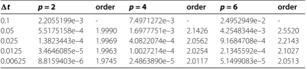
Table 1 ·2errors and convergence orders of numerical solutionuatT= 5 forp= 2, 4, and 6
t p = 2 order p = 4 order p = 6 order
0.1 2.2055199e–3 - 7.4971272e–3 - 2.4952949e–2
-0.05 5.5175158e–4 1.9990 1.6977751e–3 2.1426 4.2548344e–3 2.5520 0.025 1.3823443e–4 1.9969 4.0822074e–4 2.0562 9.1684708e–4 2.2143 0.0125 3.4646085e–5 1.9963 1.0027214e–4 2.0254 2.1345592e–4 2.1027 0.00625 8.8159403e–6 1.9745 2.4863890e–5 2.0117 5.1499083e–5 2.0513
N= to in increment of , we solve (.) up to timeT= forp= , , , respectively. The discrete norm · of numerical errors atT = is given in Figure , which shows
apparently the spatial spectral accuracy is verified.
.. Second-order accuracy in time
For exploring the temporal accuracy, we fix spatial resolution as N= , so that the numerical error is dominated mainly by the temporal ones. With a sequence of time step sizest= ., ., ., ., ., we also compute the numerical errors atT= forp= , , , respectively, and the results are presented in Table in which a second-order in time accuracy is shown clearly.
.. Conservation properties
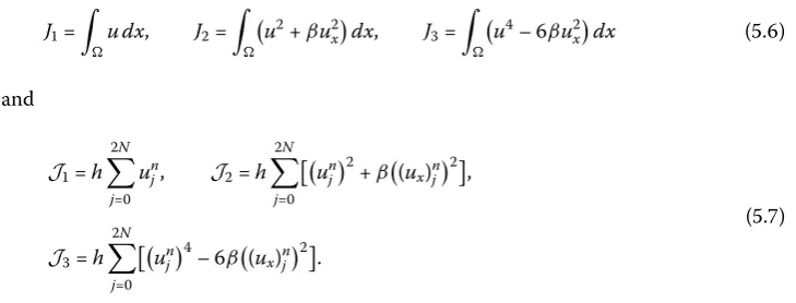
As stated in [, ], the GRLW equation has three conservative laws related to mass, momentum and energy, respectively. In particular, forp= , it reduces to the regularized long wave (RLW) equation. The invariants are given by
I=
u dx, I=
u+βuxdx, I=
u+ udx, (.)
and the corresponding discrete quantities are computed for the numerical scheme as fol-lows:
I=h N
j=
unj, I=h N
j=
unj+β(ux)nj,
I=h N
j=
unj+ unj.
Table 2 Invariants for single soliton of RLW equation withN= 128 andc=43
Time t = 0.05 t = 0.025
I1 I2 I3 I1 I2 I3
T= 0 7.9999950 5.5997821 20.266666 7.9999950 5.5997821 20.266666 T= 4 7.9999950 5.5998333 20.266871 7.9999950 5.5997884 20.266692 T= 8 7.9999950 5.5998850 20.267078 7.9999950 5.5997947 20.266717 T= 12 7.9999950 5.5999359 20.267284 7.9999950 5.5998002 20.266743 T= 16 7.9999950 5.5998258 20.267490 7.9999950 5.5996448 20.266768
Table 3 Invariants for single soliton of MRLW equation withN= 128 andc=43
Time t = 0.05 t = 0.025
J1 J2 J3 J1 J2 J3
T= 0 7.9999950 5.5997821 2.0584499 7.9999950 5.5997821 2.0584499 T= 4 7.9999950 5.5998333 2.0586695 7.9999950 5.5997884 2.0584982 T= 8 7.9999950 5.5998850 2.0588246 7.9999950 5.5997947 2.0585311 T= 12 7.9999950 5.5999359 2.05886249 7.9999950 5.5998002 2.0585384 T= 16 7.9999950 5.5998258 2.0598310 7.9999950 5.5996448 2.0595023
Taket= . andt= . withN= andc=.xL,xR,α,βare also defined as in Section .. The invariantsI,I, andIup to timeT= are given in Table .
Another special case of the GRLW equation is the modified regularized long wave (MRLW) equation withp= . Similar to the quantities for the RLW equation, the MRLW equation also has the following conservative laws:
J=
u dx, J=
u+βuxdx, J=
u– βuxdx (.)
and
J=h N
j=
unj, J=h N
j=
unj+β(ux)nj,
J=h N
j=
unj– β(ux)nj.
(.)
In Table , we presented that the discrete mass, momentum and energy of the numeri-cal solutions for the MRLW equation. From both tables, it is obvious that the proposed scheme is satisfactorily conservative.
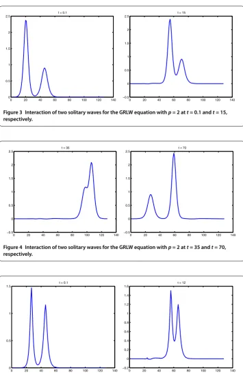
5.3 Interaction of two GRLW solitary waves
Next, we study the interaction of two well-separated solitary waves having different am-plitudes and traveling in the same direction. The initial condition is given by
u(x) =
i=
Aisechp–Ki(x+xi). (.)
Forp= , we choosec= .,c= .,x= ,x= ,t= .,N= , andα,βare
Figure 3 Interaction of two solitary waves for the GRLW equation withp= 2 att= 0.1 andt= 15, respectively.
Figure 4 Interaction of two solitary waves for the GRLW equation withp= 2 att= 35 andt= 70, respectively.
Figure 5 Interaction of two solitary waves for the GRLW equation withp= 6 att= 0.1 andt= 12, respectively.
of the GRLW equation. Meanwhile, we briefly plot two figures to show the simulation for p= att= . andt= in Figure .
Soli-man []. Moreover, the solitary-wave interaction in Figure forp= shows clearly some evidence of an additional disturbance, which may be due to the fact that the GRLW equa-tion are not completely integrable.
5.4 Unstable solitary-wave solution
Souganidis and Strauss [] derived the following result for the GRLW equation: (a) ifp< , thenu(x,t) isH-stable;
(b) ifp> , thenu(x,t) isH-stable forc>cp, andH-unstable for ≤c≤cp, where
cp= + √
–σ–+ σ–
(σ+ ) , (.)
andσ =p–. Note thatcp= whenp= andcp> forp≥. Certainly, forp= , the critical speed iscp= ..
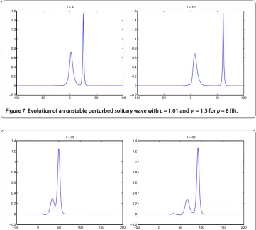
Similar to the experiments in [], the high accuracy scheme we proposed also can simu-late this phenomenon, that is, the evolution of solutions emanating from initial data which are perturbations of exact analytical solutions of (.) withp> and ≤c≤cpare featured, where the initial data is a perturbed solitary wave,
˜
u=γu(x), (.)
andγ is called the perturbation parameter; it is used to effect an amplitude perturbation. According to [], whenγ ≥, the solution emanating from the initial data will resolve itself into one or more solitary waves, sometimes accompanied by additional structure. Therefore, mainly attention will be given to evolutions starting withu˜forγ> .
Since unstable solutions have a speedcin the range ≤c≤cpandcpis near , we simu-late only one of long-time outcomes for perturbed unstable solitary-wave solutions, with
α=β= ,p= ,c= .. To achieve such an outcome, the initial unstable solitary data had
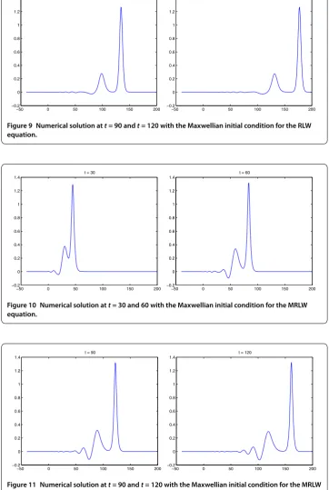
to be given enough energy to produce two stable solitary waves. Hence, we chooseγ = .. As seen in Figure and Figure , the outcomes illustrate how such a process occurred in the experiment.
Figure 7 Evolution of an unstable perturbed solitary wave withc= 1.01 andγ= 1.5 forp= 8 (II).
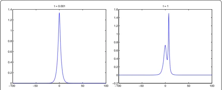
Figure 8 Numerical solution att= 30 andt= 60 with the Maxwellian initial condition for the RLW equation.
5.5 Maxwellian initial condition
A more interesting test case for the GRLW equation is to investigate the long-time asymp-totic properties by initiating the wave motion with a Gaussian pulse, namely, the so-called Maxwellian initial condition []. We takeα=,β= for RLW equation (p= ) andα=,
β= for MRLW equation (p= ), respectively, with initial data
u(x, ) =exp–.(x– ). (.) In a numerical test, letN= ,t= .,xL= –, andxR= . The numerical so-lution at different times for both cases are drawn in Figure and Figure for the RLW equation, and Figure and Figure for the MRLW equation, respectively. Furthermore, the quantities for three conservative laws are presented in Table . As seen from these results, an initial date with Maxwellian disturbance will resolve into a sequence of solitary waves in the stable range ordered by amplitude with the larger waves in the front, followed by a dispersive tail. Clearly, the presented results are consistent with earlier work on this topic in [, ].
6 Conclusion
con-Figure 9 Numerical solution att= 90 andt= 120 with the Maxwellian initial condition for the RLW equation.
Figure 10 Numerical solution att= 30 and 60 with the Maxwellian initial condition for the MRLW equation.
Figure 11 Numerical solution att= 90 andt= 120 with the Maxwellian initial condition for the MRLW equation.
Table 4 Invariants for single soliton of MRLW equation withN= 128 andc=43
Time RLW equation (p = 2) MRLW equation (p = 3)
I1 I2 I3 J1 J2 J3
T= 0 12.533141 9.0394281 33.822820 12.533141 9.0394281 5.2036174 T= 2 12.533141 9.0394599 33.823003 12.533141 9.0394430 5.2037832 T= 4 12.533141 9.0394331 33.823012 12.533141 9.0393901 5.2041213 T= 6 12.533141 9.0393867 33.823027 12.533141 9.0392994 5.2046997 T= 8 12.533141 9.0393237 33.823048 12.533141 9.0391822 5.2054479 T= 10 12.533141 9.0392517 33.823072 12.533141 9.0390559 5.2062565
unstable solitary wave of the GRLW equation withp≥ also be simulated, as established in [].
Competing interests
The authors declare that they have no competing interests.
Authors’ contributions
All authors conceived of the study, participated in its design and coordination, drafted the manuscript, participated in the sequence alignment, and read and approved the final manuscript.
Author details
1School of Science, Southwest University of Science and Technology, Mianyang, 621010, P.R. China.2School of Business, Sichuan University, Chengdu, 610064, P.R. China.
Acknowledgements
The authors are very grateful to both reviewers for carefully reading this paper and their comments, and thank Dr. Cheng Wang (University of Massachusetts, Dartmouth) for his valuable discussion. This work is supported by the Applied Basic Research Project of Sichuan Province (No. 2013JY0096) and the National Natural Science Foundation of China (No. 11202175).
Received: 16 May 2015 Accepted: 22 October 2015 References
1. Peregrine, DH: Long waves on beach. J. Fluid Mech.27(4), 815-827 (1967)
2. Benjamin, TB, Bona, JL, Mahony, JJ: Model equations for long waves in nonlinear dispersive systems. Philos. Trans. R. Soc. Lond. A272(1220), 47-78 (1972)
3. Miller, JR, Weinstein, MI: Asymptotic stability of solitary waves for the regularized long-wave equation. Commun. Pure Appl. Math.49(4), 399-441 (1996)
4. Wazwaz, AM: Analytic study on nonlinear variants of the RLW and the PHI-four equations. Commun. Nonlinear Sci. Numer. Simul.12(3), 314-327 (2007)
5. Soliman, AA: Numerical simulation of the generalized regularized long wave equation by He’s variational iteration method. Math. Comput. Simul.70(2), 119-124 (2005)
6. Zhang, L: A finite difference scheme for generalized regularized long-wave equation. Appl. Math. Comput.168(2), 962-972 (2005)
7. Chang, Q, Wang, G, Guo, B: Conservative scheme for a model of nonlinear dispersive waves and its solitary waves induced by boundary motion. J. Comput. Phys.93(2), 360-375 (1991)
8. Zheng, K, Hu, J: High-order conservative Crank-Nicolson scheme for regularized long wave equation. Adv. Differ. Equ.
2013, Article ID 287 (2013)
9. Hu, J, Zheng, K, Zheng, M: Numerical simulation and convergence analysis of a high-order conservative difference scheme for SRLW equation. Appl. Math. Model.38(23), 5573-5581 (2014)
10. Akbari, R, Mokhtari, R: A new compact finite difference method for solving the generalized long wave equation. Numer. Funct. Anal. Optim.35(2), 133-152 (2014)
11. Sloan, DM: Fourier pseudospectral solution of the regularized long wave equation. J. Comput. Appl. Math.36(2), 159-179 (1991)
12. Djidjeli, K, Price, WG, Twizell, EH, Cao, Q: A linearized implicit pseudo-spectral method for some model equations: the regularized long wave equations. Commun. Numer. Methods Eng.19(11), 847-863 (2003)
13. Roshan, T: A Petrov-Galerkin method for solving the generalized regularized long wave (GRLW) equation. Comput. Math. Appl.63(5), 943-956 (2012)
14. Achouri, T, Ayadi, M, Omrani, K: A fully Galerkin method for the damped generalized regularized long-wave (DGRLW) equation. Numer. Methods Partial Differ. Equ.25(3), 668-684 (2009)
15. Achouri, T, Omrani, K: Numerical solutions for the damped generalized regularized long-wave equation with a variable coefficient by Adomian decomposition method. Commun. Nonlinear Sci. Numer. Simul.14(5), 2025-2033 (2009)
17. Mokhtari, R, Mohammadi, M: Numerical solution of GRLW equation using Sinc-collocation method. Comput. Phys. Commun.181(7), 1266-1274 (2010)
18. Mohammadi, M, Mokhtari, R: Solving the generalized regularized long wave equation on the basis of a reproducing kernel space. J. Comput. Appl. Math.235(14), 4003-4014 (2011)
19. Souganidis, PE, Strauss, WA: Instability of a class of dispersive solitary waves. Proc. R. Soc. Edinb. A114, 195-212 (1990) 20. Bona, JL, McKinney, WR, Restrepo, JM: Stable and unstable solitary-wave solutions of the generalized regularized
long-wave equation. J. Nonlinear Sci.10(6), 603-638 (2000)
21. Durán, A, López-Marcos, MA: Numerical behaviour of stable and unstable solitary waves. Appl. Numer. Math.42(1), 95-116 (2002)
22. Boyd, J: Chebyshev and Fourier Spectral Methods, 2nd edn. Dover, New York (2001)
23. Hesthaven, J, Gottlieb, S, Gottlieb, D: Spectral Methods for Time-Dependent Problems. Cambridge University Press, Cambridge (2007)
24. Maday, Y, Quarteroni, A: Spectral and pseudospectral approximation to Navier-Stokes equations. SIAM J. Numer. Anal.
19(4), 761-780 (1982)
25. Tadmor, E: Convergence of spectral methods to nonlinear conservation laws. SIAM J. Numer. Anal.26(1), 30-44 (1989) 26. Tadmor, E: The exponential accuracy of Fourier and Chebyshev differencing methods. SIAM J. Numer. Anal.23(1),
1-10 (1986)
27. Weinan, E: Convergence of Fourier methods for Navier-Stokes equations. SIAM J. Numer. Anal.30(3), 650-674 (1993) 28. Guo, BY, Zou, J: Fourier spectral projection method and nonlinear convergence analysis for Navier-Stokes equations.
J. Math. Anal. Appl.282(2), 766-791 (2003)
29. Gottlieb, S, Wang, C: Stability and convergence analysis of fully discrete Fourier collocation spectral method for 3-D viscous Burgers’ Equation. J. Sci. Comput.53(1), 102-128 (2012)
30. Cheng, K, Feng, W, Gottlieb, S, Wang, C: A Fourier pseudospectral method for the ‘good’ Boussinesq equation with second-order temporal accuracy. Numer. Methods Partial Differ. Equ.31(1), 202-224 (2015)
31. Du, Q, Guo, B, Shen, J: Fourier spectral approximation to a dissipative system modeling the flow of liquid crystals. SIAM J. Numer. Anal.39(3), 735-762 (2001)
32. Canuto, C, Quarteroni, A: Approximation results for orthogonal polynomials in Sobolev spaces. Math. Comput.
38(157), 67-86 (1982)
33. Baskara, A, Lowengrub, JS, Wang, C, Wise, SM: Convergence analysis of a second order convex splitting scheme for the modified phase field crystal equation. SIAM J. Numer. Anal.51(5), 2851-2873 (2013)
34. Mokhtari, R, Ziaratgahi, ST: Numerical solution of RLW equation using integrated radial basis functions. Appl. Comput. Math.10(3), 428-448 (2011)