The implicit midpoint method for Riesz tempered fractional diffusion equation with a nonlinear source term

R E S E A R C H

Open Access

The implicit midpoint method for Riesz

tempered fractional diffusion equation with a

nonlinear source term

Dongdong Hu

_{and Xuenian Cao}

*_{Correspondence:[email protected]} 1_{School of Mathematics and}

Computational Science, Hunan Key Laboratory for Computation and Simulation in Science and Engineering, Xiangtan University, Xiangtan, P.R. China

Abstract

In this paper, the implicit midpoint method is presented for solving Riesz tempered fractional diffusion equation with a nonlinear source term, where the tempered fractional partial derivatives are evaluated by the modified second-order Lubich tempered difference operator. Stability and convergence analyses of the numerical method are given. The numerical experiments demonstrate that the proposed method is effective.

Keywords: Riesz tempered fractional diffusion equation; Implicit midpoint method; Stability; Convergence

1 Introduction

In this paper, we consider Riesz tempered fractional diffusion equation with a nonlinear source term

∂u(x,t)

∂t =κ

∂α,λu(x,t)

∂|x|α +g

x,t,u(x,t), (x,t)∈(a,b)×(0,T], (1.1)

with the initial and boundary conditions

u(x, 0) =ϕ(x), x∈[a,b], (1.2)

u(a,t) = 0, u(b,t) = 0, t∈[0,T], (1.3)

where 1 <α< 2,λ≥0, the diffusion coefficientκ is a positive constant,ϕ(x) is a known sufficiently smooth function,g(x,t,u) satisfies the Lipschitz condition

_g(x,t,u) –g(x,t,υ)≤L|u–υ|, ∀u,υ∈R, (1.4)

hereLis Lipschitz constant, and the Riesz tempered fractional derivative ∂α,_∂λu_|x(_|xα,y,t) is

ex-pressed as [1,2]

∂α,λ_u(x,t)

∂|x|α =cα

_R

aDαx,λ+RxD

α,λ

b

u(x,t), (1.5)

wherecα= –_2cos1₍π α 2 ),

R

aDαx,λandRxD

α,λ

b stand for the left and right Riemann–Liouville

tem-pered fractional derivatives which are defined as

R

aDαx,λu(x,t) =RaDx(α,λ)u(x,t) –λαu(x,t) –αλα–1 ∂u(x,t)

∂x , (1.6)

R xD

α,λ

b u(x,t) = R xD

(α,λ)

b u(x,t) –λ

α

u(x,t) +αλα–1∂u(x,t)

∂x , (1.7)

where the symbolsR aD

(α,λ) x andRxD

(α,λ)

b are defined by

R aD(

α,λ)

x u(x,t) =e–

λxR aD

α

xe

λx_{u(x,t) =} e–

λx

Γ(2 –α)

∂2 ∂x2

x

a

eλξu(ξ,t)(x–ξ)1–α

dξ,

R xD

(α,λ)

b u(x,t) =e

λxR

xDαbe–λxu(x,t) = eλx Γ(2 –α)

∂2 ∂x2

b

x

e–λξ_{u(ξ,t)(ξ–x)}1–α_dξ,

whereΓ(·) is Gamma function.

Moreover, ifλ= 0, then the Riesz tempered fractional derivative will reduce to the usual Riesz fractional derivative (see e.g. [3–8]).

In recent years, differential equations with tempered fractional derivatives have widely been used for modeling many special phenomena, such as geophysics [9–11] and finance [12,13] and so on. It has attracted many authors’ attention in constructing the numeri-cal algorithm for tempered fractional partial differential equation (see e.g., [1,2,14–24]). Li and Deng proposed the tempered weighted and shifted Grünwald–Letnikov formula with second-order accuracy for Riemann–Liouville tempered fractional derivative in [24], and its approximation is applied in the numerical simulation of the tempered fractional Black–Scholes equation for European double barrier option by Zhang et al. [14]. Based on this approximation, Qu and Liang [15] constructed a Crank–Nicolson scheme for a class of variable-coefficient tempered fractional diffusion equation, and disscussed the stabil-ity and convergence. Yu et al. [16] proposed a third-order difference scheme for one side Riemann–Liouville tempered fractional diffusion equation and given the stability and con-vergence analysis. Yu et al. [19] constructed a fourth-order quasi-compact difference oper-ator for Riemann–Liouville tempered fractional derivative and tested its effectiveness by numerical experiment. Zhang et al. [1] presented a modified second-order Lubich tem-pered difference operator for approximating the Riemann–Liouville temtem-pered fractional derivative and verified its effectiveness by theoretical analysis and numerical results. The aim of this paper is to try to use the implicit midpoint method and the modified second-order Lubich tempered difference operator to construct a new numerical scheme, and to give a theoretical analysis of the numerical method.

The outline of this paper is arranged as follows. In Sect.2, numerical scheme is proposed for solving Riesz tempered fractional diffusion equation with a nonlinear source term. Section3 is devoted into the stability and convergence analysis. In Sect.4, we use the proposed method (abbr. T-ML2) and the method (abbr. T-WSGL) in literature [24] to solve

the test problems. Finally, we draw the conclusion in Sect.5.

2 Numerical method

To discretize the Riemann–Liouville tempered fractional derivatives, we would intro-duce the modified second-order Lubich tempered difference operatorsδα

x–andδαx+at the

then we have the following lemma.

Lemma 2.1 ([1])Ifu(x,tn)∈Cλ2+α(R) (1≤n≤N),for the fixed step size h,we have

The fractional Sobolev spaceC2+α

λ (R)is defined by

wherev()is represented as the Fourier transformation of v(x)defined by

where

δα_x=κcα

δ_xα_–+δ_xα₊. (2.2)

Using the implicit midpoint method to solve (1.1) at the point (xi,tn), we find

u(xi,tn+1) =u(xi,tn) +τ κ ∂α,λ

∂|x|α

u(xi,tn+1) +u(xi,tn)

2

+τg

xi,t_n+1 2,

u(xi,tn+1) +u(xi,tn)

2

+Oτ3,

1≤i≤M– 1, 0≤n≤N. (2.3)

Applying (2.1) to discretize the Riesz tempered fractional derivative, we get

u(xi,tn+1) =u(xi,tn) +τ δxα

u(xi,tn+1) +u(xi,tn)

2

+τg

xi,tn+1₂,

u(xi,tn+1) +u(xi,tn)

2

+τRn+ 1 2 i ,

1≤i≤M– 1, 0≤n≤N– 1, (2.4)

where there exists a constantc1such that

_Rn+1₂ i ≤c1

τ2+h2, 1≤i≤M– 1, 0≤n≤N– 1. (2.5)

Omitting the error termRn+

1 2

i , we obtain the following numerical scheme for solving

(1.1)–(1.3):

un_i+1=un_i +τ δ_xαun+ 1 2 i +τg

n+1₂

i , 1≤i≤M1– 1, 0≤n≤N– 1, (2.6)

u0

i =ϕ(xi), 0≤i≤M, (2.7)

un₀= 0, un_M= 0, 0≤n≤N, (2.8)

whereun+ 1 2 i =

un+1 i +uni

2 ,g n+1₂

i =g(xi,tn+12,u n+1₂ i ).

Furthermore, the matrix form of (2.6) can be written as

(I–A)Un+1= (I+A)Un+τgn+12_{, 0}≤_n≤_{N– 1, (2.9)}

where

Un=un₁,un₂, . . . ,u_Mn_–1T, gn+12 _=gn+ 1 2 1 ,g

n+12 2 , . . . ,g

n+12 M–1

T

hereAis a Toeplitz matrix, which can be written asA=B+BT_{, where the matrixBis}

Remark 2.1 In [24], Li and Deng combined the Crank–Nicolson method with a tem-pered weighted and shifted Grünwald–Letnikov operator to propose a numerical method with the accuracy ofO(τ2_+h2_{) for tempered fractional diffusion equation with a}

lin-ear source term, where the tempered weighted and shifted Grünwald–Letnikov operators with second-order accuracy are defined as

δα_x–u(xi,tn) =

in the following three sets:

(1) Sα

3 Stability and convergence analysis

In order to analyze the stability and convergence of the numerical method, we would in-troduce some notations and lemmas.

for any un_,vn_∈γ

h, we define the following discrete inner product and corresponding

norm:

i is the numerical solution for (2.6)–(2.8) starting from another initial value

Proof According to (2.6), we obtain the following equation:

Employing Lemma3.1, we find

Sincegsatisfies Lipschitz condition with respect tou, we have

1

We can obtain the recursion from (3.6),

(1 –τL)ηn+12≤(1 –τL)η02+ 2τL

It follows from (3.8) and the discrete Gronwall inequality that

ηn+12_≤

e2(n+1)μτLη02

Therefore

Proof Subtracting (2.6) from (2.4), we get the error equation

εn_i+1=ε_in+τ δα_xεn+

Similarly, we can conclude from the deduction of Theorem3.1that

1

According to (1.4) and Cauchy–Schwarz inequality, we obtain from (3.10)

≤2τL

We can obtain the recursion from (3.12),

In view of the discrete Gronwall inequality, we have

εn+12_≤ τ

It follows from (2.5) and the definition of the discrete norm that

4 Numerical experiments

Denoteε(h,τ)=

hτN_n=1M_i=1–1|u(xi,tn) –un_i|2 _asL

2 norm of the error at the point

(xi,tn), whereu(xi,tn) anduni are the exact solution and numerical solution with the step

sizeshandτ at the grid point (xi,tn), respectively. The observation order is defined as

Rate =log₂

ε(2h, 2τ)

ε(h,τ)

.

Example1 Consider the initial-boundary value problem in the following Riesz tempered fractional diffusion equation:

⎧ ⎪ ⎪ ⎨ ⎪ ⎪ ⎩

∂u(x,t)

∂t =

∂α,λ_u(x,t)

∂|x|α +g(x,t,u(x,t)), x∈(0, 1),t∈(0, 1], u(x, 0) =x2_{(1 –x)}2_{, x∈[0, 1],}

u(0,t) =u(1,t) = 0, t∈[0, 1],

where 1 <α< 2, the nonlinear source term is

gx,t,u(x,t)=u(x,t)2–x2(1 –x)2e–t

+ e

–t

2cos(π α

2 )

e–λx

∞

k=0 4

m=2

λk_{Γ(k+m+ 1)Am} Γ(k+ 1)Γ(k+m+ 1 –α)x

k+m–α

+eλx–λ

∞

k=0 4

m=2

λkΓ(k+m+ 1)Am

Γ(k+ 1)Γ(k+m+ 1 –α)(1 –x)

k+m–α

– 2λαx2(1 –x)2

–x4(1 –x)4e–2t,

whereA2= 1,A3= –2,A4= 1.

The exact solution of Example1is

u(x,t) =x2(1 –x)2e–t.

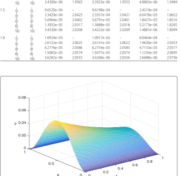
From Table1, we can observe the second-order accuracy in both spatial and temporal directions with differentαandλ, which is in line with our convergence analysis. The nu-merical solutions of Example1are shown in Fig.1, we can find from Fig.2that the global perturbation errors depend on the initial perturbation errors, which proved the correct-ness of our stability analysis.

Example2 Consider the initial-boundary value problem in the following Riesz tempered fractional diffusion equation:

⎧ ⎪ ⎪ ⎨ ⎪ ⎪ ⎩

∂u(x,t)

∂t =

∂α,λ_u(x,t)

∂|x|α +g(x,t), x∈(0, 1),t∈(0, 1],

u(x, 0) = 0, x∈[0, 1],

Table 1 Errors and corresponding observation orders of T-ML2in spatial and temporal directions for

Example1with differentαandλ

α h τ λ= 0 λ=₁₀₀1 λ= 1

ε(h,τ) Rate ε(h,τ) Rate ε(h,τ) Rate

1.2 ₁₀1 ₁₀1 7.6335e–04 – 7.5126e–04 – 1.1638e–03 –

1 20

1

20 1.9911e–04 1.9388 1.9631e–04 1.9362 2.8958e–04 2.0068

1 40

1

40 5.1544e–05 1.9497 5.0882e–05 1.9479 7.3198e–05 1.9841

1 80

1

80 1.3313e–05 1.9530 1.3155e–05 1.9516 1.8860e–05 1.9565

1 160

1

160 3.4300e–06 1.9565 3.3923e–06 1.9553 4.8865e–06 1.9484

1.5 1

10 1

10 9.6520e–04 – 9.6198e–04 – 2.4219e–04 –

1 20

1

20 2.3429e–04 2.0425 2.3357e–04 2.0421 6.6478e–05 1.8652

1 40

1

40 5.6964e–05 2.0402 5.6791e–05 2.0401 1.8427e–05 1.8510

1 80

1

80 1.3932e–05 2.0317 1.3888e–05 2.0318 5.2173e–06 1.8205

1 160

1

160 3.4330e–06 2.0208 3.4222e–06 2.0209 1.4881e–06 1.8099

1.8 ₁₀1 ₁₀1 1.0924e–03 – 1.0917e–03 – 8.0464e–04 –

1 20

1

20 2.6152e–04 2.0625 2.6141e–04 2.0622 1.9630e–04 2.0353

1 40

1

40 6.2776e–05 2.0586 6.2754e–05 2.0585 4.7153e–05 2.0577

1 80

1

80 1.5082e–05 2.0574 1.5077e–05 2.0574 1.1234e–05 2.0695

1 160

1

160 3.6282e–06 2.0555 3.6268e–06 2.0556 2.6688e–06 2.0736

Figure 1Numerical solutions for Example1withh=τ= 0.01,α= 1.5,λ= 1

where 1 <α< 2, the linear source termg(x,t) is

g(x,t) = (2 +α)t1+αe–λxx4(1 –x)4+ t

2+α

2cos(π α

2 )

e–λx 4

m=0

(–1)m_m4 Γ(5 +m)

Γ(5 +m–α)x

4+m–α

+eλ(x–2)

∞

j=0

(2λ)j

Γ(j+ 1)

4

m=0

(–1)m_m4 Γ(5 +m+j)

Γ(5 +m+j–α)(1 –x)

4+m+j–α

– 2λαe–λx_x4_{(1 –x)}4

Figure 2Numerical solutions for the perturbation equations of Example1withh=τ= 0.01,α= 1.5,λ= 1 and the initial perturbation errorη0

i = 1e– 04 (0≤i≤M)

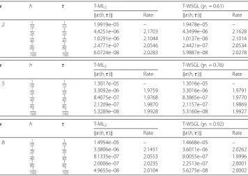
Table 2 Errors and corresponding observation orders withλ= 1, and the parametersγ1,γ2,γ3are

selected inSα₁(γ1,γ2,γ3)

α h τ T-ML2 T-WSGL (γ1= 0.61)

ε(h,τ) Rate ε(h,τ) Rate

1.2 ₁₀1 ₁₀1 1.9919e–05 – 1.9478e–05 –

1 20

1

20 4.4251e–06 2.1703 4.3499e–06 2.1628

1 40

1

40 1.0291e–06 2.1044 1.0137e–06 2.1014

1 80

1

80 2.4771e–07 2.0546 2.4421e–07 2.0534

1 160

1

160 6.0724e–08 2.0283 5.9887e–08 2.0278

α h τ T-ML2 T-WSGL (γ1= 0.76)

ε(h,τ) Rate ε(h,τ) Rate

1.5 ₁₀1 ₁₀1 1.3017e–05 – 1.3016e–05 –

1 20

1

20 3.3092e–06 1.9759 3.3016e–06 1.9791

1 40

1

40 8.4075e–07 1.9768 8.3865e–07 1.9770

1 80

1

80 2.1209e–07 1.9870 2.1157e–07 1.9869

1 160

1

160 5.3289e–08 1.9928 5.3160e–08 1.9927

α h τ T-ML2 T-WSGL (γ1= 0.92)

ε(h,τ) Rate ε(h,τ) Rate

1.8 ₁₀1 ₁₀1 1.4954e–05 – 1.4668e–05 –

1 20

1

20 3.3806e–06 2.1451 3.6011e–06 2.0262

1 40

1

40 8.1335e–07 2.0553 9.0055e–07 1.9996

1 80

1

80 2.0006e–07 2.0235 2.2513e–07 2.0001

1 160

1

160 4.9655e–08 2.0104 5.6275e–08 2.0002

The exact solution of Example2is

For contrast, we apply our numerical scheme (2.6)–(2.8) (T-ML2) and the method

(T-WSGL) in [24] for solving Example2with differentαandλ= 1, respectively. The errors and corresponding observation orders are listed in Table2, we find that T-ML2and

T-WSGL are both effective for solving Example2. However, we need to select the values ofγ1,γ2andγ3 for differentα when T-WSGL is used. In a sense, T-ML2 may be more

convenient than T-WSGL for Example2.

5 Conclusion

In this paper, the implicit midpoint method is proposed for solving the Riesz tempered fractional diffusion equation with a nonlinear source term, the numerical scheme is proved to be stable and convergent by the energy method, and numerical examples verify the correctness of the theoretical analysis and the effectiveness of the proposed method.

Acknowledgements

The authors would like to express the thanks to the anonymous referees for their valuable comments and suggestions.

Funding

This work is supported by National Science Foundation of China (No. 11671343), and the Project of Scientific Research Fund of Hunan Provincial Science and Technology Department (No. 2018WK4006).

Availability of data and materials

The authors declare that all data and material in the paper are available and veritable.

Competing interests

The authors declare that they have no competing interests.

Authors’ contributions

The two authors contributed equally and significantly in writing this article. The authors wrote, read, and approved the final manuscript.

Publisher’s Note

Springer Nature remains neutral with regard to jurisdictional claims in published maps and institutional affiliations.

Received: 3 August 2018 Accepted: 23 January 2019

References

1. Zhang, Y., Li, Q., Ding, H.: High-order numerical approximation formulas for Riemann–Liouville (Riesz) tempered fractional derivatives: construction and application (I). Appl. Math. Comput.329, 432–443 (2018)

2. Çelik, C., Duman, M.: Finite element method for a symmetric tempered fractional diffusion equation. Appl. Numer. Math.120, 270–286 (2017)

3. Li, C., Zeng, F.: Numerical Methods for Fractional Calculus, pp. 170–174. Chapman & Hall, Boca Raton (2015) 4. Liao, H., Lyu, P., Vong, S.: Second-order BDF time approximation for Riesz space-fractional diffusion equations. Int. J.

Comput. Math.95, 144–158 (2017)

5. Wang, P., Huang, C.: An implicit midpoint difference scheme for the fractional Ginzburg–Landau equation. J. Comput. Phys.312, 31–49 (2016)

6. Ding, H., Li, C.: High-order numerical algorithms for Riesz derivatives via constructing new generating functions. J. Sci. Comput.71, 759–784 (2017)

7. Choi, Y., Chung, S.: Finite element solutions for the space-fractional diffusion equation with a nonlinear source term. Abstr. Appl. Anal.2012, 183 (2012)

8. Çelik, C., Duman, M.: Crank–Nicolson method for the fractional diffusion equation with the Riesz fractional derivative. J. Comput. Phys.231, 1743–1750 (2012)

9. Baeumer, B., Meerschaert, M.: Tempered stable Lévy motion and transient super-diffusion. J. Comput. Appl. Math.

233, 2438–2448 (2010)

10. Meerschaert, M., Zhang, Y., Baeumer, B.: Tempered anomalous diffusion in heterogeneous systems. Geophys. Res. Lett.35, L17403 (2008)

11. Metzler, R., Klafter, J.: The restaurant at the end of the random walk: recent developments in the description of anomalous transport by fractional dynamics. J. Phys. A, Math. Gen.37, R161 (2004)

12. Carr, P., Geman, H., Madan, D., Yor, M.: Stochastic volatility for Lévy processes. Math. Finance13, 345–382 (2003) 13. Wang, W., Chen, X., Ding, D., Lei, S.: Circulant preconditioning technique for barrier options pricing under fractional

diffusion models. Int. J. Comput. Math.92, 2596–2614 (2015)

15. Qu, W., Liang, Y.: Stability and convergence of the Crank–Nicolson scheme for a class of variable-coefficient tempered fractional diffusion equations. Adv. Differ. Equ.2017, 108, 1–11 (2017)

16. Yu, Y., Deng, W., Wu, Y., Wu, J.: Third order difference schemes (without using points outside of the domain) for one sided space tempered fractional partial differential equations. Appl. Numer. Math.112, 126–145 (2017)

17. Dehghan, M., Abbaszadeh, M.: A finite difference/finite element technique with error estimate for space fractional tempered diffusion-wave equation. Comput. Math. Appl.75, 2903–2914 (2018)

18. Wu, X., Deng, W., Barkai, E.: Tempered fractional Feynman–Kac equation: theory and examples. Phys. Rev. E93, 032151 (2016)

19. Yu, Y., Deng, W., Wu, Y., Wu, J.: High-order quasi-compact difference schemes for fractional diffusion equations. Commun. Math. Sci.15, 1183–1209 (2017)

20. Zayernouri, M., Ainsworth, M., Karniadakis, G.: Tempered fractional Sturm–Liouville EigenProblems. SIAM J. Sci. Comput.37, A1777–A1800 (2015)

21. Chen, M., Deng, W.: High order algorithms for the fractional substantial diffusion equation with truncated Lévy flights. SIAM J. Sci. Comput.37, A890–A917 (2015)

22. Sabzikar, F., Meerschaert, M., Chen, J.: Tempered fractional calculus. J. Comput. Phys.293, 14–28 (2015)

23. Zheng, M., Karniadakis, G.: Numerical methods for SPDEs with tempered stable processes. SIAM J. Sci. Comput.37, A1197–A1217 (2015)