A simple model for mantle-driven flow at the top of Earth’s core
Hagay Amit1, Julien Aubert2, Gauthier Hulot1, and Peter Olson3
1Equipe de G´eomagn´etisme, Institut de Physique du Globe de Paris (Institut de Recherche associ´e au CNRS eta l’Universit´e Paris 7),` 4 Place Jussieu, 75252 Paris Cedex 05, France
2Equipe de Dynamique des Syst`emes G´eologiques, Institut de Physique du Globe de Paris 3Department of Earth and Planetary Sciences, Johns Hopkins University, Baltimore, MD 21218, USA
(Received November 15, 2007; Revised April 7, 2008; Accepted April 26, 2008; Online published September 8, 2008)
We derive a model for the steady fluid flow at the top of Earth’s core driven by thermal coupling with the heterogeneous lower mantle. The model uses a thermal wind balance for the core flow, and assumes a proportionality between the horizontal density gradients at the top of the core and horizontal gradients in seismic shear velocity in the lowermost mantle. It also assumes a proportionality between the core fluid velocity and its radial shear. This last assumption is validated by comparison with numerical models of mantle-driven core flow, including self-sustaining dynamo (supercritical) models and non-magnetic convection (subcritical) models. The numerical dynamo models show that thermal winds with correlated velocity and radial shear dominate the boundary-driven large-scale flow at the top of the core. We then compare the thermal wind flow predicted by mantle heterogeneity with the 150 year time-average flow obtained from inverting the historical geomagnetic secular variation, focusing on the non-zonal components of the flows because of their sensitivity to the boundary heterogeneity. Comparing magnitudes provides an estimate of the ratio of lower mantle seismic anomalies to core density anomalies. Comparing patterns shows that the thermal wind model and the time-average geomagnetic flow have comparable length scales and exhibit some important similarities, including an anticlockwise vortex below the southern Indian and Atlantic Oceans, and another anticlockwise vortex below Asia, suggesting these parts of the non-zonal core flow could be thermally controlled by the mantle. In other regions, however, the two flows do not match well, and some possible reasons for the dissimilarity between the predicted and observed core flow are identified. We propose that better agreement could be obtained using core flows derived from geomagnetic secular variation over longer time periods.
Key words:Thermal wind, mantle tomography, time-average core flow, geodynamo.
1.
Introduction
Convection in the outer core is likely influenced by the heterogeneous thermal boundary conditions imposed on the core by the overlying mantle. Evidence for this mantle in-fluence is sometimes found in paleomagnetic and archeo-magnetic field models in the form of long-term departures from axial symmetry (Gubbins and Kelly, 1993; Johnson and Constable, 1995; Constableet al., 2000; Korteet al., 2005), but not always (McElhinnyet al., 1996; Carlut and Courtillot, 1998; Hongreet al., 1998) because such depar-tures are difficult to identify unambiguously (Bouligandet
al., 2005; Hulot and Bouligand, 2005; Khokhlov et al.,
2006). In this paper we focus on historical time-scales to assess the influence of the overlying lower mantle on the current working of the geodynamo. More specifically, we study core flows rather than the geomagnetic field itself be-cause the time-scale of flow variations is shorter than the time-scale of the geomagnetic field (Hulot and LeMou¨el, 1994; Le Huyet al., 2000), potentially giving better chances of identifying steady features by averaging core flows over historical times than by averaging the geomagnetic field.
Copyright cThe Society of Geomagnetism and Earth, Planetary and Space Sci-ences (SGEPSS); The Seismological Society of Japan; The Volcanological Society of Japan; The Geodetic Society of Japan; The Japanese Society for Planetary Sci-ences; TERRAPUB.
We therefore explore the possibility that flows driven by the heterogeneous lower mantle could explain some of the cen-tral features found in time-average core surface flow models accounting for the historical geomagnetic secular variation. The latter flow models testify for significant asymmetries within the core. First, most of the core flow activity, as well as the secular variation, occurs in the Atlantic hemisphere, while the Pacific hemisphere remains much quieter (Amit and Olson, 2006). Second, core flow models averaged over 150 years display significant north-south asymmetry, with strong westward drift at low and mid-latitudes of the south-ern hemisphere, but much less drift in the northsouth-ern hemi-sphere (Pais and Hulot, 2000; Amit and Olson, 2006). Do these asymmetries merely reflect transient short time-scale features of the geodynamo, or could they indeed be caused by the heterogeneity of the overlying mantle?
It has already been proposed that heterogeneous mantle boundary conditions could control some of the fluid motion in the outer core (Bloxham and Gubbins, 1987). Most re-cent studies relied on numerical simulations and assumed thermal boundary conditions related to seismic shear ve-locity anomalies in the lower mantle (see Aubert et al., 2007, and references therein). According to this assump-tion, a high/low seismic shear velocity anomaly at the lower mantle correlates with a dense/light (cold/hot) lower mantle
(Yuenet al., 1993; Forte and Mitrovica, 2001), and there-fore a high/low heat flux across the core-mantle boundary. This for instance led Olson and Christensen (2002) to find that long-term time-average flows in full 3D self-consistent numerical dynamos with such tomographic boundary con-ditions are indeed affected by both mantle-driven and in-ternal core dynamical effects, and as a result, display more westward drift in the southern than in the northern hemi-sphere, as well as a large anti-clockwise vortex below the southern Atlantic and Indian Oceans. These are akin to similar features seen in short-term time-average core flow models derived from geomagnetic secular variation mod-els (Pais and Hulot, 2000; Amit and Olson, 2006). More recently, Aubertet al. (2007) used numerical dynamos to study the likelihood of identifying mantle control on core flows averaged over such short time periods, namely three vortex turnover times which they claim is equivalent to 100–360 years of observations. Their results show that a significant signature of mantle-driven thermal wind can be expected in core flows averaged over such short periods. Aubert et al.(2007), however, did not directly assess the extent to which the time-average core flow computed from the historical geomagnetic data displays the kind of features expected from mantle controlled core flow. The purpose of this study is precisely to look into this in details.
To infer the expected signature of mantle control on core surface flows we use a simple model starting from thermal wind theory, which relies on a vorticity balance at the top of the core dominated by effects of rotation (Section 2). In addition, we assume that thermal boundary conditions im-posed by the mantle induce lateral density gradients at the top of the core proportional to the seismic shear velocity pattern in the lower mantle. Those density gradients drive a thermal wind flow which we further assume has a radial shear proportional to the flow itself. This approach has al-ready been used by Amit and Olson (2006) to examine man-tle control on their zonal time-average core flow inferred from the geomagnetic secular variation. They found that the north-south asymmetry in mid-latitudes of the zonal ge-omagnetic flow is qualitatively similar to that of the zonal thermal wind, and may therefore be an indication to mantle control. However, the difficulty in separating the effects of the homogeneous dynamo flow and the mantle-driven flow might interfere with such an interpretation. Here we focus on the non-zonal component of the flow, which best reflects the signature of mantle control (by avoiding back-ground zonal dynamo flows unrelated to mantle control). This mantle-driven thermal wind flow model is first vali-dated with the help of flow models derived from numeri-cal dynamos (Section 3). It is next used for comparisons with the time-average core flow model of Amit and Olson (2006) based on geomagnetic secular variation inversions (Section 4). This finally allows us to discuss the possi-bility that thermal control of the mantle could be responsi-ble for some of the features found in the time-average core flow model inferred from 150 years of geomagnetic data, as Aubertet al.(2007) suggested could be the case.
2.
Mantle-driven Thermal Wind Flow Model
In a spherical coordinate system (r, θ, φ), where r is the distance from Earth’s center, θ is co-latitude andφ is longitude, the standard thermal wind equation for a thick fluid shell just below the core-mantle boundary(r = R)is (Pedlosky, 1987)whereu is velocity,zis the direction of the rotation axis, g0 andρ0 are gravitational acceleration and density at the
core-mantle boundary respectively,is rotation rate,ρ is the laterally-variable density andrˆis the radial unit vector. In spherical coordinates (1) can be rewritten as
cosθ∂u
Our goal is to solve for the velocity components on the left hand sides of (3)–(4) given some knowledge ofρ (which we will later infer independently). The second term on the left hand sides of (3)–(4) (the meridional gradient of the flow, ∂uφ/∂θ and∂uθ/∂θ) can be integrated for a given density pattern provided the first term on the left hand sides of (3)–(4) (the radial shear ∂uφ/∂r and∂uθ/∂r) is known. Unfortunately this is not directly the case. To our best knowledge, there is neither a general analytical solu-tion to (3)–(4), nor a general theoretical relasolu-tion between the radial shear and the flow. However, and as we will later show, numerical dynamos suggest a very convenient ap-proximate proportionality between the mantle-driven flow and its radial shear at the top of the core:
∂uh
∂r L
−1uh
R (5)
whereL−1is a non-dimensional parameter. Substituting (5) into (3)–(4), the thermal wind at the top of the core is then approximated by
Table 1. Global vector correlation coefficientCs between non-zonal radial shear∂∂urh
nz
and non-zonal normalized flow uh
R
nz
at the top of the free stream (r =0.938 forE =3·10−4andr =0.905 forE =6·10−4) and their ratioL−1. Also given the high-latitudes correlation coefficients C45for latitudes higher than 45◦andC60for latitudes higher than 60◦. The global correlation coefficientCcis between the non-zonal radial shear term cosθ∂uh
∂r
nz
and the non-zonal normalized flow term cosθuh
R
nz
and their ratio isL−1
c . Finally, a global correlation coefficientCρbetween the
non-zonal imposed boundary heat flux and the non-zonal density at the top of the free stream is also given. The correlation coefficients are calculated as the averaged scalar product of the two vectors normalized by their averaged magnitudes. The ratiosL−1andL−1
c are calculated as the best-fit
global linear regression. The parameters used in the dynamo simulations are the Rayleigh (Ra), Ekman (E), Prandtl (Pr) and magnetic Prandtl (Pm) numbers. The magnitude of the heat flux anomaly imposed on the outer boundary isq∗defined as the ratio of peak-to-peak to mean heat flux. All cases have tomographic boundary conditions, except casesY2
2 andY21that have corresponding single-harmonic boundary conditions. All cases have
been time-averaged over several magnetic diffusion times. All cases are supercritical dynamos exceptSwhich is subcritical. All dynamos are dipolar exceptT2.
assume that the density anomaly at the top of the core is it-self proportional to this heterogeneous heat flux (Gubbins, 2003; Amit and Olson, 2006). These imply the following linear relationship between horizontal density gradients at the top of the core and horizontal shear wave velocity gra-dients at the base of the mantle:
1
wherevs is seismic shear wave velocity in the mantle,ρ0
is the mean outer core density, andCis a constant of pro-portionality. Because the constantC is a priori unknown, in this study mainly flow patterns will be investigated. An estimate ofCwill nevertheless be derived.
In practice, in order to estimate the thermal wind core surface flow associated with a given pattern of seismic shear velocity anomalies at the lowermost mantle, we use (8) to inferρ, and (6)–(7) to infer the tangential velocity compo-nents. We use a central finite-difference numerical method on a regular 5◦ ×5◦ grid. The solution is obtained by a standard matrix inversion scheme. For more details includ-ing boundary conditions see Appendix A. We finally focus on the non-zonal component of this model, and we term it from hereafter thethermal wind model.
3.
Model Validation
The thermal wind model heavily relies on two important assumptions, formulated as (5) and (8). To assess the valid-ity of those assumptions, several tests can be performed us-ing numerical dynamos subjected to heterogeneous bound-ary conditions (for a detailed description of the numerical dynamo model we use, see Aubertet al., 2007). The pat-tern of imposed heat flux on the outer boundary is either based on the lower mantle tomography model of Masterset al.(2000) (truncated at degree 8 to consider only robust fea-tures) or implemented as a single-harmonic boundary con-dition. In all cases, we examine flows at the top of the free stream below the Ekman boundary layer, at the depth at
which viscous forces become negligible in the force bal-ance. For the simulations discussed here this corresponds to about 3.5–4hek(wherehek=
√
E Dis the Ekman bound-ary layer thickness, E is the Ekman number and D is the shell thickness). Those flows are next long-term time aver-aged to isolate the steady flow. As already stated, we also restrict ourselves to the non-zonal part of the flow to avoid the purely zonal long-term time-average dynamo homoge-neous flow (Aubert, 2005) and to focus on mantle-driven core flow features.
For each simulation we assess the validity of (5) by com-paring the resultingunzh /Rflow with its radial shear∂unzh /∂r
and computing correlation coefficients and best-fit linear regression values (Table 1). The global correlations be-tween the non-zonal radial shear of the flow∂unzh/∂rto the
non-zonal tangential flow itselfunzh /Rat the top of the free
stream for casesT1lq,T0,T1,T1hpandY1
2 are well above
the 95% significance level, which is about 0.2 for the res-olution of the numerical dynamos in this study (Rauet al., 2000). When only high-latitudes are considered, the cor-relations are high for all cases. For the highest 45◦ lati-tudes all cases yield 0.66 > C45 > 0.42, and the range is
0.76> C60 >0.66 for the highest 60◦ latitudes. It is
im-portant to stress that the inferior correlation at low-latitudes is not a major issue for thermal wind modelling because the radial shear term is less important at low-latitudes. Indeed, comparing maps of the relevant quantities for thermal wind modelling, the non-zonal radial shear term cosθ∂unzh /∂r
and the non-zonal tangential flow term cosθunzh /R(Fig. 1),
reveals good global pattern agreement for both tangential components. The global correlations between these two terms are high for all cases, 0.64 > Cc > 0.34 (Table 1).
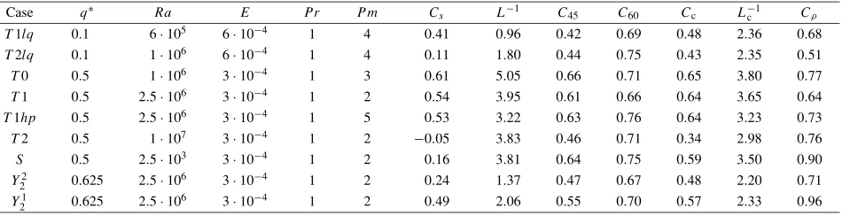
bound-Fig. 1. (a) Non-zonal time-average radial shear of azimuthal flow term cosθ∂∂urφnz; (b) Normalized non-zonal time-average azimuthal flow term cosθL−R1uφnz; (c) Non-zonal time-average radial shear of meridional flow term cosθ∂∂urθnz; (d) Normalized non-zonal time-average meridional flow term cosθLR−1uθnz. All maps are for caseT1 (see Table 1) at the top of the free stream (r =0.938). Red/blue denotes eastward/westward radial shears (a) and flows (b), or southward/northward radial shears (c) and flows (d). All quantities are in dimensionless units.
ary. The high positive correlations reported here are typi-cally found between depths of∼0.05–0.2D(or∼3–12hek),
including just below the Ekman boundary layer, the rele-vant depth for comparison with the time-average core flow computed from the geomagnetic data.
The approximate relation (5) holds for the time-average non-zonal part of the flow because of permanent radial plumes that form at the top of the core as a result of convection driven from above. This produces tangential velocities which reach their radial peak value just below the outer boundary layer. Indeed, radial profiles of non-zonal radial and non-non-zonal tangential time-average flows (not shown here) generally contain intense radial flows in mid-shell which convert to increasing tangential flows when approaching the outer boundary.
Some cases satisfy (5) globally whereas others tend to fail at low-latitudes. Figure 2 compares arbitrary longitu-dinal slices of cases T2, T1, T0 andY2
2. Cases T0 and
T1 satisfy (5) globally because the plumes driven from above extend radially and the azimuthal velocities peak be-low the Ekman layer at all latitudes. In case T2 the ve-locities peak too deep at low-latitudes due to the strong mixing which breaks the radial plumes. Note that in this regime the dynamo is anyway non-dipolar (Kutzner and Christensen, 2002). In case Y22 the perfect equatorially-symmetric boundary condition favors rotational effects and
the plumes extend along the z-direction rather than radi-ally. However, the assumption holds well at all latitudes for the corresponding more relevant multi-harmonic boundary conditions case.
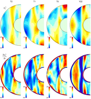
Another even more direct way of validating the relevance of the radial shear assumption (5) of the resulting Eqs. (6) and (7) consists in comparing the flows that those equations predict, with the numerical dynamo flows. This is done in Fig. 3 which shows two types of flows. The right column shows non-zonal time-average flows at the top of the core for four numerical dynamos with heterogeneous heat flux boundary conditions based on the lower mantle tomogra-phy model of Masterset al.(2000). The first flow model
(the subcritical flowcase S, Fig. 3(f)) is obtained from a
T1
T2 T0 Y22
160
-160 40
-40
60
-60 15
-15
20
-20 5
-5
60
-60 15
-15
Fig. 2. Longitudinal slices of non-zonal time-average azimuthal flowunz
φ (top) and non-zonal time-average radial shear of azimuthal flow∂ uφ ∂r
nz
(bottom) for casesT2,T1,T0 andY2
2. Red/blue denotes eastward/westward flows or radial shears in dimensionless units. All slices are at the same longitude.
column of Fig. 3 shows those thermal wind flows with their driving densityρ. They very nicely show that if a correct knowledge ofρ at the top of the free stream is available, relying on both the thermal wind Eqs. (3)–(4) and the ra-dial shear assumption (5) to derive and use (6)–(7), allows to very closely predict the correct flow.
What about assumption (8)? This assumption also can be tested against numerical dynamos. Figure 3(j) shows the full lowermost mantle seismic shear velocity anomalies based on the tomographic model of Masters et al.(2000) which was used to impose the heat flux on the outer bound-ary for the numerical dynamos. Those led to the subcrit-ical and dynamo steady flows shown in Figs. 3(f)–(i) and to the corresponding non-zonal density distributions shown in Figs. 3(a)–(d). Thus, checking that (8) is sensible essen-tially amounts to checking that the non-zonal tomographic pattern in Fig. 3(e) matches the non-zonal density patterns in Figs. 3(a)–(d). That is not exactly the case. Although all those density patterns have much in common (seeCρ val-ues in Table 1), clear differences can be seen which trans-late into similar differences in the corresponding flow pat-terns (e.g. compare Figs. 3(c) and (h)). In particular, not
all flow patterns display details such as the shift of about 15◦ to the east in some southern hemisphere features with respect to their northern counterparts, which appear in the thermal wind model. Those are clearly related to the fact that (8) intrinsically implies some locking of the density pattern with respect to the heterogeneous heat flux bound-ary conditions we impose. Assumption (8) thus appears to be the weakest of the several assumptions our thermal wind model requires. This in fact, is not quite a surprise. Indeed, Olson and Christensen (2002) already found in numerical dynamos with aY2
2 boundary heat flux that the flow pattern
0.24 -0.24
Tomographic thermal wind with L =3 0.06
-0.06
S
T0
T1
0.04 -0.04
0.02 -0.02
T2
Dynamo flows Thermal winds driven by dynamo densities with L =3-1
-1
%
Full tomographic boundary conditions for the numerical dynamos
1.78 -1.78
rms = 85
rms = 150
rms = 350
rms = 145
rms = 150
rms = 600
(e) (j)
(a) (f)
(b) (g)
(c) (h)
(d) (i)
%
2.47 -2.47
Fig. 3. Mantle-driven models of non-zonal core flow. (a)–(d): Non-zonal density at the top of the free stream from numerical dynamos, with superimposed streamfunction contours of the non-zonal thermal wind models forL−1 =3 and using those numerical dynamos non-zonal density.
(f)–(i): The respective subcritical and dynamo steady flows. In (a)–(d) and (f)–(i): Contour intervals were adjusted for clear visualizations, flow rms of each column is given relative to caseS((a) and (f) respectively). The cases from top to bottom areS,T0,T1 andT2 (see Table 1). Black/grey contours denote anticlockwise/clockwise circulation, respectively. (e): Non-zonal seismic shear velocity model at lowermost mantle (Masterset al., 2000) truncated at spherical harmonic degree 8, with superimposed streamfunction contours of the non-zonal thermal wind model forL−1 = 3.
Contour intervals were adjusted for clear visualizations. (j): Full seismic shear velocity model at lowermost mantle (Masterset al., 2000) truncated at spherical harmonic degree 8 used as a heat flux boundary condition for the numerical dynamos. In (e) and (j): Blue is positiveδvs/vs anomaly
(b)
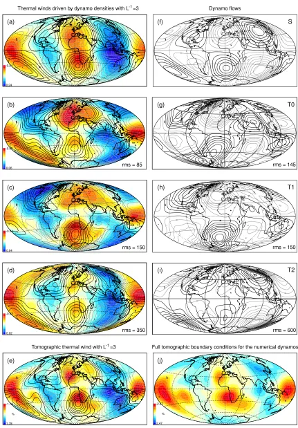
(c) Geomagnetic flow
Thermal wind L =3 rms=1.6
-1
(a) Thermal wind L =10-1
Fig. 4. Streamfunction of the non-zonal thermal wind model forL−1=10
(a) andL−1=3 (b), and the non-zonal time-average geomagnetic flow
((c), maximum velocity is 24.5 km/year, rms is 6.1 km/year). Flow rms in (b) is given relative to (a). In all maps black/grey contours denote anticlockwise/clockwise circulation, respectively. The vector correlation between (b) and (c) is 0.11.
for investigating the influence of lower mantle thermal het-erogeneity on the time-average non-zonal flow at the top of the core. We must however acknowledge that the differ-ences seen among the various dynamo steady flows in Fig. 3 are likely reflections of the uncertainties one should expect for modelling mantle-driven flow with numerical dynamos, because of the limited computational ability to model the geodynamo process in the appropriate parameter regime.
It finally remains to point out that the choice of the value of the parameterL−1remains arbitrary. We choseL−1 =3
for the results shown in Fig. 3 motivated by our numerical dynamos (Table 1). But we also tried several other values. A larger value ofL−1results in a weaker flow but does not
much affect the pattern (see Figs. 4(a) and (b)). We con-clude that the pattern of the thermal wind model is robust and does not depend greatly on our choice of the model pa-rameterL−1.
4.
Comparison with Time-average Flow Inferred
from Geomagnetism
We now compare the non-zonal thermal wind model with the non-zonal time-average core flow model of Amit and
Olson (2006) obtained from inversions of the geomagnetic secular variation modelgufm1(Jackson et al., 2000) over the period 1840–1990 (Fig. 4(c), from hereafter the geo-magnetic flow). We chose this time interval since geomag-netic data prior to 1840 is considered less reliable because full magnetic vector measurements were not performed then. This flow model was obtained by solving the frozen-flux radial magnetic induction equation using a helical-geostrophic assumption (Amit and Olson, 2004, 2006) and averaging over the 150 years time period. The parameters used for this computation (k = 0.15 and c = 1) imply superimposed tangential geostrophy and helical flow con-straints to ensure formal uniqueness of the solution. This, we note in Appendix B, is compatible with the thermal wind assumption. It leads to main flow features which are any-way also seen in other core flow models obtained from ge-omagnetic secular variation data using different approaches (Bloxham, 1989; Jacksonet al., 1993; Holme, 1998; Chul-liat and Hulot, 2000; Pais and Hulot, 2000; Hulot et al., 2002; Eymin and Hulot, 2005). Comparison between our thermal wind model (Fig. 4(b)) and the geomagnetic flow (Fig. 4(c)) reveals important agreements but also some dis-crepancies.
Main features in the non-zonal time-average geomag-netic flow include (1) a large anticlockwise vortex in mid-and high-latitudes of the southern hemisphere below the Indian and Atlantic Oceans, (2) a clockwise vortex below North America, (3) an anticlockwise vortex below Asia, and (4) a more active Atlantic hemisphere than the Pacific one. These features are quite persistent throughout the pe-riod considered, the rms of the non-zonal time-dependent part of the flow being only 30% of the rms of the non-zonal time-average flow.
Comparison with the thermal wind model shows that two of the main large-scale geomagnetic flow vortices are re-covered by the thermal wind model in terms of both center and direction of circulation. The anticlockwise vortex be-low the Indian and Atlantic Oceans in the geomagnetic flow (Fig. 4(c)) is similar to the one found below the Southern Atlantic in the thermal wind model (Fig. 4(b)). The vortex below Asia associated with the high density mantle struc-ture there is also in good agreement between the thermal wind model and the geomagnetic flow. In contrast, some flow features found in the thermal wind model, such as the vortex below North America, clearly disagree with the geo-magnetic flow.
%
1.78 -1.78
(a) Observed lower mantle
heterogeneity
(b) Predicted lower mantle
heterogeneity
Fig. 5. Lower mantle density heterogeneity based on the observed seismic shear velocity tomographic model of Masterset al.(2000) (a), and the forward calculated density based on the geomagnetic flow and the thermal wind model (b). Blue is positive anomaly (dense, cold), red is negative (light, hot).
combination with the larger eastward shift in the southern hemisphere of the geomagnetic flow, result in good agree-ment between the thermal wind model and the geomagnetic flow over the eastern hemisphere of the core-mantle bound-ary, but relatively poor agreement over the western hemi-sphere.
Another interesting comparison can be made between the observed lower mantle seismic heterogeneity (which we as-sume drives the thermal wind) and the lower mantle seis-mic heterogeneity the geomagnetic flow would predict from Eqs. (6), (7) and (8) (Fig. 5). Regions of agreement in-clude cold structures below the western limb of the Pacific rim and warm structures below the southern Atlantic, but discrepancies are also apparent, for example below North America where a seismic cold region is in disagreement with the forward calculated warm region. Overall, the spa-tial distribution of regions of agreement and discrepancy in heterogeneities (Fig. 5) is similar to the comparison of the two flow models (Fig. 4), with more agreement in the east-ern hemisphere than in the westeast-ern hemisphere.
What could be the reasons for such discrepancies? First, thermal wind could of course be an oversimplified theory for steady core flow. Although our analysis of numerical dynamos suggests that the thermal wind balance is well-satisfied, whether this also holds for the Earth’s core can still be questioned. Second, the input we use for the ther-mal core-mantle boundary conditions is clearly simplified and idealized. Part of the buoyancy in the lower mantle may be attributed to chemical (Trampert et al., 2004) or mineralogical (Murakamiet al., 2004) anomalies. Third, various problems associated with core flow inversions from geomagnetic data (Bloxham and Jackson, 1991; Eymin and Hulot, 2005; Holme, 2007), especially nonuniqueness
is-sues, might result in inaccurate core flow models for com-parison with thermal wind models. In this respect, and as pointed out to us by R. Holme (personnal communication), the extent to which the steady part of a flow model inferred from geomagnetic data could be found with a driving den-sity forced to be significantly close to that inferred from lower mantle seismology, would clearly be worth investi-gating further. Finally, the time interval used for averaging the geomagnetic flow, 150 years, might still be too short.
All of the above discussion was based on comparisons of flow patterns and ignored the value of the parameterC in (8). We may now infer an estimate ofC based on our thermal wind model. By constraining rms magnitudes for the thermal wind model and the geomagnetic flow to be equal, and using=7.29·10−5s−1andg
0 =10.68 m s−2
(Dziewonsky and Anderson, 1981), we findC ∼2.7·10−7.
This value is consistent withδvs/vs ∼ 2·10−2 (Masters
et al., 2000) while the Boussinesq approximation on the core side requiresδρ/ρ0 = αδT with thermal expansivity
α ∼ 10−5K s−1 (Poirier, 2000) and temperature anomaly
δT ∼10−3K (Bloxham and Gubbins, 1987).
In summary, we have introduced a simple thermal wind model to predict the steady flow at the top of the core from heterogeneous boundary conditions imposed by the lower mantle. This thermal wind model has been validated us-ing numerical dynamos. It provides an easy way to inves-tigate the likely signature of thermal boundary conditions imposed by the mantle. Using the model of Masters et al.(2000) to infer thermal mantle heterogeneity, the ther-mal wind model shares several important features with a time-average flow inferred from 150 years of geomagnetic data (Amit and Olson, 2006). Discrepancies might orig-inate from incomplete interpretation of the seismic data, uncertainties in core flow modelling, or insufficient time-averaging of the geomagnetic core flow. Future progress in modelling mantle tomography, geomagnetic secular varia-tion and core flow may provide further insight to the under-standing of core-mantle interactions and the steady flow in the core.
Acknowledgments. Numerical calculations were performed at the Service de Calcul Parallelle, IPGP. H. A. was supported by a grant from the IntraEuropean MarieCurie Action. We thank Richard Holme and Alexandra Pais for their useful reviews. This is IPGP contribution 2384.
Appendix A. Method
We calculate the right hand side of (6)–(7) using the man-tle density model and the thermal core-manman-tle coupling as-sumption (8). We solve for each flow component using a matrix inversion method. At the closest latitudes to the poles we use the smallness of sinθto neglect the meridional derivative terms, and by that we avoid a problem of unde-fined polar velocities in spherical coordinates. To avoid nu-merical instabilities at the equator, we solve for each hemi-sphere separately by setting a matching boundary condition at the equator. For the azimuthal velocity, we use the exact form of (7) at the equator,
−∂uθ ∂θ |eq=
g0
2ρ0
∂ρ
Our goal is to find the (main) toroidal flow, so we assume
Combining (A.1) and (A.2) we get the approximated bound-ary condition for the azimuthal flow:
uφ|eq=
g0
2ρ0
ρ|eq (A.3)
For the meridional velocity, we setuθ|eq =0 at the
equa-tor, which is the exact solution to the radial component of the thermal wind, generally known as the tangential geostrophic constraint.
Introducing θi = θ0 +iδ from θ0 = 2.5◦ to θn =
87.5◦ with δ = 5◦, the thermal wind equation for each flow component (uφanduθ) at longitudeφin the northern hemisphere can then be discretized and written in the matrix form:
Mu =b (A.4)
whereuis either(uθ(θ0),uθ(θ1), ...uθ(θn))when
consider-ing the meridional flow componentuθ, or(uφ(θ0),uφ(θ1),
...uφ(θn))when considering the azimuthal flow component
uφ, andMis given by (accounting for the boundary condi-tions): The vectorbis then given either by
g0
equator. For each longitudeφ, and each flow componentuφ anduθ, the matrixMis tri-diagonal and therefore invertible. Solutions are then obtained through
u =M−1b (A.8)
A similar procedure is used to compute the flow in the southern hemisphere.
Appendix B. Compatibility
of
the
Helical-geostrophic
and
Thermal
Wind
Assumptions
The thermal wind equation is the 3D balance of Coriolis and buoyancy vorticities (1). Its tangential components (3) and (4) retain both contributors, but the radial buoyancy vor-ticity is identically zero, yielding the tangential geostrophic equation: ∇h ·(uhcosθ)=0. This suggests that the
ther-mal wind assumption should be more compatible with core flows derived with the tangential geostrophic assumption than with an helical-geostrophic assumption. However, nu-merical dynamos prove that the tangential components (3) and (4) of the thermal wind balance (1) (Aubert, 2005; Aubert et al., 2007) and the helical flow assumption
(Ol-sonet al., 2002; Amitet al., 2007) may both be reasonably
satisfied. In numerical dynamos, helicity is generated by a temperature field configuration that produces thermal winds with peakz-velocities close to the center of columnar vor-tices (Olsonet al., 1999). On approach to the outer surface,
the z-velocities turn to tangentially divergent flow, which
correlates with radial vorticity at the top of the free stream. The radial Coriolis vorticity is expected to be smaller than its tangential counterparts, and may be relaxed by radial vis-cous vorticity. This relaxation may lead to the shift between upwellings at centers of vortices (according to helical flow) and upwellings at the east/west limbs of vortices (according to tangential geostrophy). It is therefore reasonable to com-pare the thermal wind flow models with core flows inverted based on the helical flow assumption.
References
Amit, H. and P. Olson, Helical core flow from geomagnetic secular varia-tion,Phys. Earth Planet. Inter.,147, 1–25, 2004.
Amit, H. and P. Olson, Time-average and time-dependent parts of core flow,Phys. Earth Planet. Inter.,155, 120–139, 2006.
Amit, H., P. Olson, and U. Christensen, Tests of core flow imaging methods with numerical dynamos,Geophys. J. Int.,168, 27–39, 2007. Aubert, J., Steady zonal flows in spherical shell fluid dynamos,J. Fluid
Mech.,542, 53–67, 2005.
Aubert, J., H. Amit, and G. Hulot, Detecting thermal boundary control in surface flows from numerical dynamos,Phys. Earth Planet. Inter.,160, 143–156, 2007.
Bloxham, J., Simple models of fluid flow at the core surface derived from geomagnetic field models,Geophys. J. Int.,99, 173–182, 1989. Bloxham, J. and D. Gubbins, Thermal core-mantle interactions,Nature,
325, 511–513, 1987.
Bloxham, J. and A. Jackson, Fluid flow near the surface of the Earth’s outer core,Rev. Geophys.,29, 97–120, 1991.
Bouligand, C., G. Hulot, A. Khokhlov, and G. Glatzmaier, Statistical pale-omagnetic field modeling and dynamo numerical simulation,Geophys. J. Int.,161, 603–626, 2005.
Carlut, J. and V. Courtillot, How complex is the time-averaged geomag-netic field over the past 5 Myr?,Geophys. J. Int.,134, 527–544, 1998. Christensen, U. and P. Olson, Secular variation in numerical geodynamo
models with lateral variations of boundary heat flow,Phys. Earth Planet. Inter.,138, 39–54, 2003.
Chulliat, A. and G. Hulot, Local computation of the geostrophic pressure at the top of the core,Phys. Earth Planet. Inter.,117, 309–328, 2000. Constable, C., C. Johnson, and S. Lund, Global geomagnetic field models
for the past 3000 years: transient or permanent flux lobes?,Phil. Trans. Roy. Soc. A,358, 991–1008, 2000.
Dziewonsky, A. M. and D. L. Anderson, Preliminary reference Earth model,Phys. Earth Planet. Inter.,25, 297–356, 1981.
Eymin, C. and G. Hulot, On surface core flows inferred from satellite magnetic data,Phys. Earth Planet. Inter.,152, 200–220, 2005. Forte, A. M. and J. X. Mitrovica, Deep-mantle high-viscosity flow and
Nature,410, 1049–1056, 2001.
Gibbons, S. J. and D. Gubbins, Convection in the earths core driven by lateral variations in the core-mantle boundary heat flux,Geophys. J. Int., 142, 631–642, 2000.
Glatzmaier, G., R. Coe, L. Hongre, and P. Roberts, The role of the earth’s mantle in controlling the frequency of geomagnetic reversals,Nature, 401, 885–890, 1999.
Gubbins, D., Thermal core-mantle interactions: theory and observations, in
Earth’s Core: dynamics, structure and rotation, edited by V. Dehant, K. Creager, S. Karato, and S. Zatman, 277 pp., AGU Geodynamics Series American Geophysical Union, Washington D.C., 2003.
Gubbins, D. and P. Kelly, Persistent patterns in the geomagnetic field over the past 2.5 Myr,Nature,365, 829–832, 1993.
Holme, R., Electromagnetic core-mantle coupling—I. Explaining decadal changes in the length of day,Geophys. J. Int.,132, 167–180, 1998. Holme, R., Large-scale Flow in the Core, inTreatise on Geophysics vol. 8,
edited by Olson, P., 358 pp., Elsevier Science, London, 2007. Hongre, L., G. Hulot, and A. Khokhlov, An analysis of the geomagnetic
field over the past 2000 years,Phys. Earth Planet. Inter.,106, 311–335, 1998.
Hulot, G. and J.-L. LeMou¨el, A statistical approach to the Earth’s main magnetic field,Phys. Earth Planet. Inter.,82, 167–183, 1994. Hulot, G. and C. Bouligand, Statistical paleomagnetic field modeling and
symmetry considerations,Geophys. J. Int.,161, 591–602, 2005. Hulot, G., C. Eymin, B. Langlais, M. Mandea, and N. Olsen, Small-scale
structure of the geodynamo inferred from Oersted and Magsat satellite data,Nature,416, 620–623, 2002.
Jackson, A., J. Bloxham, and D. Gubbins, inDynamics of Earth’s deep interior and Earth rotation, edited by LeMou¨el, J.-L., D. E. Smylie, and T. Herring, 189 pp., Geophysical Monograph 72 IUGG, Washington D.C., 1993.
Jackson, A., A. R. T. Jonkers, and M. R. Walker, Four centuries of geo-magnetic secular variation from historical records,Phil. Trans. R. Soc. Lond.,A358, 957–990, 2000.
Johnson, C. and C. Constable, The time averaged geomagnetic field as recorded by lava flows over the past 5 Myr,Geophys. J. Int.,112, 489– 519, 1995.
Khokhlov, A., G. Hulot, and C. Bouligand, Testing statistical paleomag-netic field models against directional data affected by measurement er-rors,Geophys. J. Int.,167, 635–648, 2006.
Korte, M., A. Genevey, C. Constable, U. Frank, and E. Schnepp, Continuous geomagnetic field models for the past 7 millenia: 1. A new global data compilation, Geochem. Geophys. Geosyst., 6, doi:10.1029/2004GC000800, 2005.
Kutzner, C. and U. Christensen, From stable dipolar towards reversing numerical dynamos,Phys. Earth Planet. Inter.,131, 29–45, 2002. Le Huy, M., J.-L. LeMou¨el, and A. Pais, Time evolution of the fluid flow
at the top of the core. Geomagnetic jerks,Earth Planets Space,52, 163– 173, 2000.
Masters, G., G. Laske, H. Bolton, and A. Dziewonski, inEarth’s deep in-terior, edited by S. Karato, A. M. Forte, R. C. Liebermann, G. Masters, and L. Stixrude, 289 pp., AGU monograph 117, Washington D.C., 2000. McElhinny, M., P. McFadden, and R. Merrill, The time-averaged
paleo-magnetic field 0–5 ma,J. Geophys. Res.,101, 25,007–25,027, 1996. Murakami, M., K. Hirose, K. Kawamura, N. Sata, and Y. Ohishi,
Post-Perovskite Phase Transition in MgSiO3,Science,304, 855–858, 2004.
Olson, P. and U. Christensen, The time averaged magnetic field in numeri-cal dynamos with nonuniform boundary heat flow,Geophys. J. Int.,151, 809–823, 2002.
Olson, P., U. R. Christensen, and G. A. Glatzmaier, Numerical modeling of the geodynamo: mechanisms of field generation and equilibration,J. Geophys. Res.,104, 10383–10404, 1999.
Olson, P. and G. A. Glatzmaier, Magnetoconvection and thermal coupling of the Earth’s core and mantle,Phil. Trans. R. Soc. Lond.,A354, 1413– 1424, 1996.
Olson, P., I. Sumita, and J. Aurnou, Diffusive magnetic images of up-welling patterns in the core,J. Geophys. Res.,107, 2348, 2002. Pais, A. and G. Hulot, Length of day decade variations, torsional
oscilla-tions and inner core superrotation: evidence from recovered core surface zonal flows,Phys. Earth Planet. Inter.,118, 291–316, 2000.
Pedlosky, J.,Geophysical Fluid Dynamics, 710 pp., Springer, New York, 1987.
Poirier, J.-P.,Introduction to the Physics of the Earth’s Interior, 312 pp., Cambridge University Press, Cambridge, UK, 2000.
Rau, S., U. Christensen, A. Jackson, and J. Wicht, Core flow inversion tested with numerical dynamo models,Geophys. J. Int.,141, 485–497, 2000.
Trampert, J., F. Deschamps, J. Resovsky, and D. Yuen, Probabilistic Tomo-graphic Maps Chemical Heterogeneities Throughout the Lower Mantle,
Science,306, 853–856, 2004.
Yuen, D. A., O. Cadek, A. Chopelas, and C. Mtyska, Geophysical infer-ences of thermal-chemical structures in the lower mantle,Geophys. Res. Lett.,20, 899–902, 1993.