R E S E A R C H
Open Access
The stable extrinsic extended finite
element method for second order elliptic
equation with interfaces
Jianping Zhao
1,2*, Yanren Hou
3, Lina Song
4and Dongwei Gui
2*Correspondence:
[email protected] 1College of Mathematics and
System Sciences, Xinjiang University, Urumqi, 830046, China 2Cele National Station of
Observation and Research for Desert-Grassland Ecosystem, Xinjiang Institute of Ecology and Geography, Urumqi, 830011, China Full list of author information is available at the end of the article
Abstract
In this paper, a stable extrinsic extended finite element method (SXFEM) is proposed to solve the second order elliptic equation with discontinuous coefficients and interfaces. SXFEM is designed by the stable enrichment function and stress intensity factors (SIF)-type enrichment functions. It shows that the proposed SXFEM can get the optimal convergence order. Numerical experiments are presented to verify the feasibility of the new method for this type of problem and the superiority compared with the standard FEM and XFEM.
Keywords: extended finite element method; generalized finite element method;
discontinuous coefficients; extrinsic; interface
1 Introduction
We consider the boundary value problem of the form
–∇ ·(a(x,y)∇u) =f(x,y), (x,y)∈\,
u(x,y) = , (x,y)∈∂, ()
whereis a bounded domain in Rd(d= , ) with polygonal or polyhedral boundary∂, f∈L(),f ∈L(),=
iiis the internal interface that may consist of several pieces of local internal interfacesi, which are also called interfaces in what follows. Generally, any two different interfaces might be intersected, that is,i∩j=∅(i=j) is possible. The functiona(x,y)∈L∞() satisfies
<α≤a(x,y)≤β<∞, ∀(x,y)∈,
whereα,βare constants. It assumes that the functiona(x,y) is discontinuous across the in-terfaceiwhile it is continuous away from the interfaces. This interface problem appears in fluid dynamics and material science. The traditional finite difference method (FDM) and the finite element method (FEM) fail to solve such a problem due to the singularities of the interface. They need improvement to deal with such kind of interface problems. For the approximation of non-smooth solutions, there are two fundamentally different ap-proaches. One approach of the improvement is to refine the discretization near the critical
regions. Remeshing is required in this case,i.e., placing more grid-points along the inter-face and around the intersection. This strategy involvesa posteriorierror estimates. For example, Cai and Zhang [] proposed recovery-based error estimators and Bernardi and Verfürth [] proposed weighted-residual error estimators to deal with interface problems. Another strategy of improvement is to enrich a polynomial approximation space so that the non-smooth solutions can be modeled independent of the mesh. For example, the immersed boundary method (IBM) [] and the immersed interface method (IIM) [] are developed based on finite difference, and they modify the standard centered difference ap-proximation to maintain the second order accuracy [–] or to get higher order methods [, ], while the immersed finite element method (IFEM) developed in [–] is de-signed to cope with interface problem based on the finite element method (FEM). In this paper, we consider the complex interface problems such as interfaces intersecting with each other.
Meanwhile, a variety of modifications to the conventional FEM have been made within the framework of the partition of unity (PU). One typical example is the extended finite element method (XFEM). It was first realized by Belytschko and Black in [] by enriching the nodes of the finite elements near the crack tips and along the crack surfaces with the asymptotic crack tip functions. Since then, such a method received wide publicity and quick progress [–]. During the same decades, the generalized finite element method (GFEM) based on the partition of unity method (PUM) [–] was widely used to solve various types of problems. All of these methods share the property that they add special enrichment functions to a standard approximation space.
Based on and inspired by the development of these methods in [], we try to use XFEM for solving elliptic problems with interfaces. One of our goals is to make the condition number of the matrix for the discrete system comparable with FEM by extrinsic XFEM.
The rest of the paper is organized as follows. Section introduces preliminary definition related to the XFEM and the weak form of (). The main part of this paper is Section , in which the feasible stable XFEM and its error estimation are derived. The integration strat-egy for XFEM is discussed in Section , and some numerical experiments are presented in Section to show the feasibility of the proposed algorithms. A final conclusion is drawn in Section .
2 Preliminary definitions
2.1 The weak form of the problem
We use the standard notation for the Sobolev spaceHk() =Wk,() and its associated
norm · Hk()and semi-norm| · |Hk(), especiallyH() =L(). Then the weak
formu-lation of () reads as follows: findu∈H() such that
B(u,v) :=
a(x,y)∇u· ∇v dx dy=
fv dx dy= (f,v), ∀v∈H(). ()
Sincea(x,y) is bounded and away from zero, the variational problem has a unique solution. For convenience of later expression, for any subdomainA⊆, we introduce the follow-ing energy normvε(A):
vε(A)=BA(v,v), ∀v∈H(A),
2.2 The extrinsic XFEM
Letτhbe a uniform rectangular mesh of the domain, and we define the mesh parameter h> ,Nis the set of nodes on the meshτh. LetI:={i∈Z, ≤i≤N}, whereN=N(h) is an integer, which is the number of nodes in the mesh. Fori∈I, letωi⊂be the impact area ofxi. Considering the Ritz-Galerkin implementation for the XFEM for a two-dimensional elliptic equation, finite-dimensional subspacesVh⊂H(),Vh⊂H() are used as the approximating trial and test spaces. The trial functions are
uh=
Here, Ni are the finite-element shape functions,φ(x) is the level set function, ui is the numerical solution of real nodexi, andvijis the solution of virtual nodes located on xi. They are the unknown coefficients of approximation.Ien=Ihmeans that we can enrich all nodes if needed.
3 Stable extrinsic extended finite element method and error estimation
In this section we give the stable extended finite element algorithm step by step and give the estimation for L-error and energy-error.
3.1 The stable extrinsic XFEM
Subordinate to the cover{ωi}i∈Ih, let{Ni}beC-PU. We can also describe the functionuh
as anni-dimensional local approximating spaceVihon each patchωi.
Vi=span ϕijni
j=, ϕ
i
j∈H(ωi) andϕi= .
Here,niis a positive integer. Ifni= , inωhi we just use a standard FEM basis function. In other cases the local area needs a special function in order to mimic the exact solution there. The PUM form about () is precisely by (), with the finite-dimensional spaceVh given by
The extrinsic XFEM discretization of () is as follows: finduh∈Vhsuch that
Extended approximations use locally enriched nodes with the aim to capture disconti-nuities and/or high gradients, and the linear dependencies are less frequently observed and often identified easily. At last the approximations of the form () do not have the Kronecker-δproperty. Consequently,uh(xi)=uimakes the imposition of essential bound-ary conditions difficult.
Based on these problems, it is important to make () satisfy the Kronecker-δproperty and linear independence. Babuška [] proposed the idea of stabilization of GFEM. First, according to the PUM theorem in the energy norm [, ], we give the main approxima-tion result about the relaapproxima-tion between global approximaapproxima-tion and local approximaapproxima-tion. We define the modified local approximation spaceVi¯ =span{ ¯ϕji}associated withVi. Here,
¯
ϕji=ϕji–π ϕji, whereπ ϕji:= k∈{k(i)|xk(i)∈ωi}
ϕji(xk)Nk; ()
π ϕi
jis the piecewise linear interpolation ofϕijon the patchωi. Clearly,ϕ¯ij= whenj= . Then the finite-dimensional spaceS=S+S¯is a subspace ofH() withS=
i∈IhuiNi
andS¯=
i∈INiVi¯. For the example mentionedVi=P(ωi),Sremains unchanged,S¯=
span{Niϕ¯i,Niϕ¯i}. The stable XFEM to approximate the solutionuof () is given by
Finduh∈S, satisfyB(uh,v) =F(v), ∀v∈S. ()
We have the boundary conditionsu|∂= to obtain a unique solutionuh∈S. It is called stable XFEM.
Leta(x,y) in () be a piecewise constant, we will consider two situations, namelya(x,y) = a if (x,y)∈ anda(x,y) =a if (x,y)∈, where the subdomains have the interface:
∪=,∩=.
Algorithm .
(i) Suppose thatis a rectangular domain. Find the first-type enriched nodes setIen and
elements along interfaces by a level set function. The second-type enriched nodes setIen
is chosen by the impact area of intersection. Meanwhile we can easily find the two types of enriched elements.
(ii) The first-type enrichment functionMis determined by the level set functionφ(x), hereφ(x) = , ifx∈ we can useφ(x) = –minx∈x–x as a level set function and
discontinuous coefficients across the interfaces.
M(x) =φ(x). ()
If the function has strong discontinuity, we also need the enrichment functionsign(φ), so
M(x) =sign
φ(x), M(x) =φ(x). ()
For the second-type enriched node, we use the four enriched basis functions like SIFs (Stress Intensity Factors) []
F(x) =
√
rcosθ/,
F(x) =
√
rsinθ/,
F(x) =
√
rsinθsinθ/,
F(x) =
√
rsinθcosθ/.
()
(iii) Stabilization of the local approximation space. Letx∈ωi,
Mj(x) =Mj(x) –IωiMj(x), j= , ,
Fj(x) =Fj(x) –Iωi
Fj(x), j= , , , .
()
Hereωiis the abbreviation ofωhi mentioned above,Iωi(ϕ
i
j) is the piecewise linear interpo-lation ofϕi
jon the patchωi.
Iωi
ϕji= xk∈ωi
ϕji(xk)Nk(x)|ωi. ()
(v) Construction element stiff matrix is called EMAT, and the unit load vector is called ERHS. The freedoms associated were increased to six.
ψ= [N;M;F;F;F;F],
EMATi,j=
E
a∇ψi∇ψjdx dy,
ERHSj=
E
fψjdx dy.
Then we can get the whole stiff matrix and solve the finite element equation.
EMAT –→x = ERHS. ()
Here, x is the vector that equals x = (u,uen).
(vi) Output the numerical result and error.
Remark . The element stiff matrix size varies with different types of elements. The common element far away from interfaces has four freedoms, while the element near in-tersection has degrees of freedoms.
Remark . When computing the integration on the element containing intersection, we
decompose the element into several triangles by the location of intersection.
The XFEM is a PUM, where
() the piecewise linear FE hat functionNiassociated with the vertices of FE rectangu-larity serves as the PU.
Supposingu∈H
() is the solution of (), we use Q-element as the PU function.
Next we discuss the semi-definiteness of the stiff matrix of the stable XFEM. From the definition ofV, anyv∈Vhas the following:
v(x) = i∈I
uiNi(x) +
i∈I
j=
bijNi(x)ψj(x); ui,bij∈R,
whereψj(x) isM(x),Fl(x),l= , , , . For each element, we can get the single stiff matrix, B(vi,vj) =a∇vi· ∇vjdx dy. The value can be divided into three types as follows:
() Ifvi∈S,vj∈S,Bij=B(Ni,Nj), which is the basic part of XFEM, is the standard N×NFE stiffness matrix.
() If vi∈S,vj∈S orvi∈S,vj∈S, Bij= andBji= , because theS andS are
orthogonal in the inner productB(·,·).
() Ifvi∈S,vj∈S,Bij=B(Niψi,Njψj),Bis only associated with some verticesxi(j)∈ Ien or Ien. The additional degrees of freedom are introduced here. We can get the stiff matrix
A=
KU KUA KAU KA
.
It is well known that the standard FE stiffness matrix block is block-tridiagonal, and we can get the argument that the matrix blockKUis positive definite. If the matrix blockKA is also positive definite, the stiff matrixAof the stable XFEM will be positive definite.
3.2 The analysis of stable XFEM
Theorem . Let u∈H(ω
i).Suppose that for i∈Ih,there existςi∈Viand C> , inde-pendent of i,such that
u–ςiL(ω
i)≤Cdiam(ωi)u–ςiε(ωi) and u–ςiε(ωi)≤i.
Then there exists v∈V such that
u–uhε()≤inf
v∈Vu–vε()≤C
i∈Ih
i /
,
where the positive constant C depends onκ,C, αβ [, ].
It is easy to check that the argument in Theorem . holds. Actually, there existsξi∈Vi such thatu–ξiε(ωi)≤Ch|u|H(ω
i),u–ξiL(ωi)≤Ch
|u|
L(ω
i), then we can get
u–uhL()=Oh,
u–uhε()=O(h),
()
Theorem . Let u∈H()be the solution of().Suppose that for each xi,which is in the rangle element (Q) as a PU,
w–v¯=
With the similar argument and the interpolation estimate, we have
wL(ω
i)=u–πωiL(ω
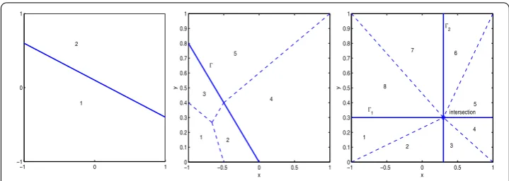
Figure 1 Dividing a fully or partially cut element into subelements, left: 2, middle: 5, right: 8.
Then we get the first term on the right-hand side of ()
xi∈I\Ien
Niw
ε()
≤C
xi∈I\Ien
u–πωi
ε().
Finally, according to (), we have
w–v¯ε()=u–πhu–v¯ε()≤C
xi∈I\Ien
u–πωiu
ε(ωi)+
xi∈Ien
i
by settingv=πhu+v¯∈S+S¯.
4 Modified numerical integration for XFEM
In standard FEM, we often use standard Gauss integration in all elements because the shape functions are smooth in the inner of the element. However, if the problem has interface, the smoothness could not be guaranteed in some elements cut by an interface. In XFEM[], give the outline of integration strategy.
In this work we first divide the special element into subelements as shown in Figure . We can find that the subelements may contain a triangle, a common quadrangle or curved edge graphics, especially if the element contains intersection of interfaces shown in the right figure of Figure . We should utilize the vertices of element, the intersection of the edge and interface, the intersection of different interfaces. In order to get more accurate integration, the subdivision uses the same number of Gauss nodes with other regular ele-ment.
This numerical integration strategy is also suitable for both extrinsic and intrinsic XFEM. If the interfaceis curve, from Figure we should first approximate it by sev-eral segments of bounding polygon and use more subdivisions in Figure . Of course we can use more segments in order to approximate the curve of interface.
5 Numerical test
We use Matlab to implement our methods. First we introduce some notations. nElem = nElemx= nElemy means we have uniform meshes in x-direction and y-direction h= /nElem,
SFEM means the standard finite element method,
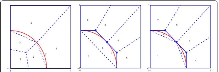
Figure 2 Dividing a fully or partially cut element into subelements, left: 2, middle: 5, right: 8.
DOF means the degrees of freedom,
u–uh: the relative L-error foruhusing SXFEM,
orderLmeans the convergence rate in L-error order,
u–uhE: the relative energy-error foruhusing SXFEM, we get the result by
u–uhE=
a(x,y)∇(u–uh)dx dy
/
a(x,y)(∇u)dx dy /
,
orderEmeans the convergence rate in energy-norm.
In this section we choose the standard benchmark test and report some numerical re-sults for an interface problem with intersecting interfaces used by many researchers, see [, , ]. Let= (–, )×(–, ), the exact solution is as follows:
u(r,θ) =rβμ(θ)
in polar coordinates at the origin with
μ(θ) = ⎧ ⎪ ⎪ ⎪ ⎨ ⎪ ⎪ ⎪ ⎩
cos(β(π
–σ))cos(β(θ–
π
+ρ)) ifθ∈[,
π
],
cos(βρ)cos(β(θ–π+σ)) ifθ∈[π,π], cos(βσ)cos(β(θ–π–ρ)) ifθ∈[π,π], cos(β(π
–ρ))cos(β(θ– π
–σ)) ifθ∈[ π
, π],
whereρ,σ are constant numbers. The exact solution satisfies (),f = anda(x,y) =Rif (x,y)∈(, )∪(–, ), anda(x,y) = if (x,y)∈\([, ]∪[–, ]). The numbersβ,R,
σ andρsatisfy nonlinear relations (e.g., [, ])
R≈., ρ=π/ and σ≈..
Here, β = ., it is a difficult problem for computation by standard FEM. The ex-act solution is singular on the origin node and the interfaces are x-axis and y-axis (fixed by the discontinuity ofa(x,y)).: (x,y)|xy= ,x≥,: (x,y)|xy= ,y≥,:
(x,y)|xy= ,x≤ and: (x,y)|xy= ,y≤ The origin node (, ) is the intersecting
in-terfaces.
In this test we use Q element, all nodes are divided into three different types as follows:
. The node with influence areaω(xi)∩i=∅;
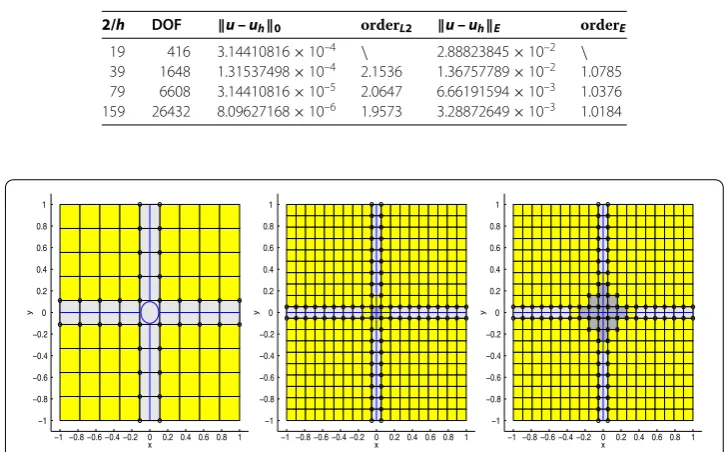
Table 1 DOF, the energy-error and L2-error using sXFEM for different step, impact radius r= 0.1
2/h DOF u – uh0 orderL2 u – uhE orderE
19 416 3.14410816×10⁻⁴ \ 2.88823845×10⁻² \
39 1648 1.31537498×10⁻⁴ 2.1536 1.36757789×10⁻² 1.0785 79 6608 3.14410816×10⁻⁵ 2.0647 6.66191594×10⁻³ 1.0376 159 26432 8.09627168×10⁻⁶ 1.9573 3.28872649×10⁻³ 1.0184
Figure 3 The mesh and interface and intersection nodes and area: left,r= 0.1,h= 2/11, middle
r= 0.1,h= 2/19 and rightr= 0.3,h= 2/19.
. Other elements. Not all the nodes in these elements need to be enriched(one, two or three nodes are enriched in some elements).
We talk about the nd-enriched nodes chosen. Table shows that the error does de-crease dramatically when the impact area inde-creases, so we can choose the impact area radiusr= . orr=√h. We just need guarantee that at least there is an element that is enriched (all nodes of the element are enrichment nodes). For example, in Figure we can choose the gray color circle area, not the left of Figure (r=hit is considered as the st enriched nodes). Table also verifies that the impact radius is not important for the development of error.
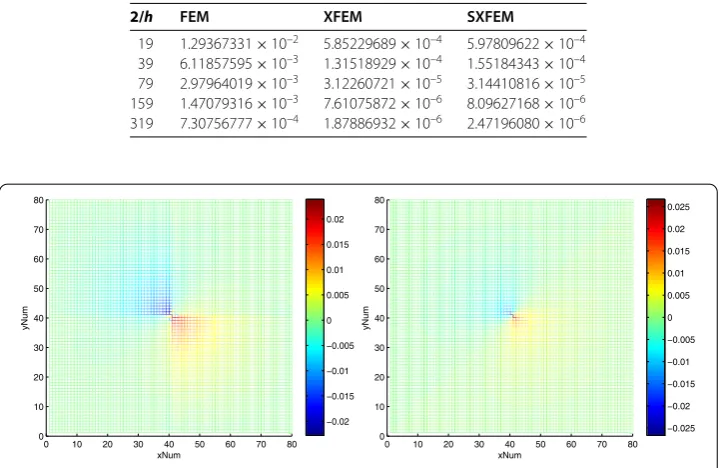
We list the numerical error by stable XFEM and DOF when the impact radius isr= . in Table . We can easily find that our method has reached the optimal orders. In Table we also list the numerical error with different impact radius, the error is not decreased when the radius is larger. Generallyr=√his enough. In the last Table , we show the L-error by FEM and XFEM and stable extrinsic XFEM with the same mesh. It is shown that the FEM only has a half of order of optimal convergence. And the intrinsic XFEM is a little better than stable XFEM.
For two types of XFEM, the L-error iso(h), and the energy-error iso(h). It is better than that of FEM, we do not list the result of the reference [] using a triangular element. According to Figure , it is shown that difference of the error distribution about FEM method and sXFEM. The result in their reference the absolute energy-error is often con-sidered to be ., while the degree of freedom is about ,. According to the results of our method numerical relative energy-error is .×–, while DOF number is
Table 2 DOF, the energy-error and L2-error using sXFEM with different impact radiusr
2/h r DOF u – uh0 u – uhE
51 0.05 2720 7.62956091×10⁻⁵ 1.03929952×10⁻² 51 0.1 2800 7.63216118×10⁻⁵ 1.03929961×10⁻² 51 0.2 3024 7.64345134×10⁻⁵ 1.03929957×10⁻² 51 0.3 3456 8.01596131×10⁻⁵ 1.03930097×10⁻²
Table 3 Comparison of L2-error (u–uh0) using standard FEM, stable XFEM and modified intrinsic XFEM
2/h FEM XFEM SXFEM
19 1.29367331×10⁻² 5.85229689×10⁻⁴ 5.97809622×10⁻⁴ 39 6.11857595×10⁻³ 1.31518929×10⁻⁴ 1.55184343×10⁻⁴ 79 2.97964019×10⁻³ 3.12260721×10⁻⁵ 3.14410816×10⁻⁵ 159 1.47079316×10⁻³ 7.61075872×10⁻⁶ 8.09627168×10⁻⁶ 319 7.30756777×10⁻⁴ 1.87886932×10⁻⁶ 2.47196080×10⁻⁶
Figure 4 Error distribution by different methods: standard FEM, stable XFEM (h= 2/79).
6 Conclusions
In this article, we discussed the stable XFEM for the second order elliptic equation with discontinuous coefficients and derivative of solutions, and it comes to the following con-clusions. Firstly we modified the local enrichment function space, and we analyzed how the global error can be dominated by the local error. It was different from the shift function only changed in vertices []. Secondly we described the stable XFEM step by step, we also gave the error estimation if we use Q- element. The L-error iso(h), and energy-error
iso(h). We also got the optimal convergence same with SXFEM. Two types of XFEM are better than FEM, to adapt the FEM result in reference [] a triangular element was used. There the absolute energy-error was considered as ., while the DOF is about ,. Numerical relative energy-error in this paper was .×–, while DOF is only
,. We will extend our method in general area, and it can be used to different meshes and high order polynomials. At last we gave the numerical simulation for the standard benchmark example. Numerical results support our analysis, we get the optimal order for energy-error and L-error, respectively.
Competing interests
Authors’ contributions
All authors contributed equally to the writing of this paper. All authors read and approved the final manuscript.
Author details
1College of Mathematics and System Sciences, Xinjiang University, Urumqi, 830046, China.2Cele National Station of
Observation and Research for Desert-Grassland Ecosystem, Xinjiang Institute of Ecology and Geography, Urumqi, 830011, China.3School of Mathematics and Statistics, Xi’an Jiaotong University, Xi’an, 710049, China.4School of Mathematics Science, Qingdao University, Qingdao, 266071, China.
Acknowledgements
The authors of this work are grateful to the journal editors and the anonymous reviewers for their comments and recommendations, which have greatly improved our manuscript and made it more suitable for readers of the journal. This work is subsidized by China Postdoctoral Science Foundation funded project (No. 2014M562487) and NSFC of China (Nos. 11461068, 11171269, 11401332, 61163027, 11362021).
Received: 28 November 2014 Accepted: 25 May 2015 References
1. Cai, ZQ, Zhang, S: Recovery-based error estimator for interface problems: conforming linear elements. SIAM J. Numer. Anal.47, 2132-2156 (2009)
2. Bernardi, C, Verfürth, R: Adaptive finite element methods for elliptic equations with non-smooth coefficients. Numer. Math.85, 579-608 (2000)
3. Peskin, CS: Numerical analysis of blood flow in heart. J. Comput. Phys.25, 220-252 (1977)
4. Leveque, RJ, Li, ZL: The immersed interface method for elliptic equations with discontinuous coefficients and singular sources. SIAM J. Numer. Anal.31, 1019-1044 (1994)
5. Fogelson, AL, Keener, JP: Immersed interface methods for Neumann and related problems in two and three dimensions. SIAM J. Sci. Comput.22, 1630-1684 (2000)
6. Li, Z, Ito, K, Lai, M-C: An augmented approach for Stokes equations with a discontinuous viscosity and singular forces. Comput. Fluids36, 622-635 (2007)
7. Huang, H, Li, Z: Convergence analysis of the immersed interface method. IMA J. Numer. Anal.19, 583-608 (1999) 8. Wiegmann, A, Bube, KP: The explicit-jump immersed interface method: finite difference methods for PDEs with
piecewise smooth solutions. SIAM J. Numer. Anal.37(3), 827-862 (2000)
9. Berthelsen, PA: A decomposed immersed interface method for variable coefficient elliptic equations with non-smooth and discontinuous solutions. J. Comput. Phys.197, 364-386 (2004)
10. Zhao, JP, Hou, YR, Li, YF: Immersed interface method for elliptic equations based on a piecewise second order polynomial. Comput. Math. Appl.63, 957-965 (2012)
11. Xia, KL, Zhan, M, Wei, G-W: The matched interface and boundary (MIB) method for multi-domain elliptic interface problems. J. Comput. Phys.230, 8231-8258 (2011)
12. Zhou, YC, Zhao, S, Feig, M, Wei, GW: High order matched interface and boundary method for elliptic equations with discontinuous coefficients and singular sources. J. Comput. Phys.213, 1-30 (2006)
13. Pan, KJ, Tan, YJ, Hu, HL: An interpolation matched interface and boundary method for elliptic interface problems. J. Comput. Appl. Math.234, 73-94 (2010)
14. Li, Z: The immersed interface method using a finite element formulation. Appl. Numer. Math.27, 253-267 (1998) 15. Xie, H, Li, Z, Qiao, Z: A finite element method for elasticity interface problems with locally modified triangulations. Int.
J. Numer. Anal. Model.8, 189-200 (2011)
16. Lin, T, Lin, Y, Zhang, X: A method of lines based on immersed finite elements for parabolic moving interface problems. Adv. Appl. Math. Mech.5(4), 548-568 (2013)
17. Lin, T, Sheen, D: The immersed finite element method for parabolic problems with the Laplace transformation in time discretization. Int. J. Numer. Anal. Model.10(2), 298-313 (2013)
18. He, XM, Lin, T, Lin, YP: Immersed finite element methods for elliptic interface problems with non-homogeneous jump conditions. Int. J. Numer. Anal. Model.8, 284-301 (2011)
19. Belytschko, T, Black, T: Elastic crack growth in finite elements with minimal remeshing. Int. J. Numer. Methods Eng.45, 601-620 (1999)
20. Moës, N, Dolbow, J, Belytschko, T: A finite element method for crack growth without remeshing. Int. J. Numer. Methods Eng.46, 131-150 (1999)
21. Sukumar, N, Chopp, DL, Moës, N, Belytschko, T: Modeling holes and inclusions by level sets in the extended finite-element method. Comput. Methods Appl. Mech. Eng.190, 6183-6200 (2001)
22. Chessa, J, Wang, H, Belytschko, T: On the construction of blending elements for local partition of unity enriched finite elements. Int. J. Numer. Methods Eng.57, 1015-1038 (2003)
23. Wu, JY: Unified analysis of enriched finite elements for modeling cohesive cracks. Comput. Methods Appl. Mech. Eng.
200, 3031-3051 (2011)
24. Babuška, I, Melenk, JM: The partition of unity method. Int. J. Numer. Methods Eng.40, 727-758 (1997)
25. Melenk, JM, Babuška, I: The partition of unity finite element method: basic theory and application. Comput. Methods Appl. Mech. Eng.139, 289-314 (1997)
26. Babuška, I, Banerjee, U: Stable generalized finite element method (SGFEM). Comput. Methods Appl. Mech. Eng.201, 91-111 (2012)
27. Liu, XY, Xiao, QZ, Karihaloo, BL: XFEM for direct evaluation of mixed mode SIFs in homogeneous and bi-materials. Int. J. Numer. Methods Eng.59, 1103-1118 (2004)
28. Fries, TP, Belytschko, T: The intrinsic XFEM: a method for arbitrary discontinuities without additional unknowns. Int. J. Numer. Methods Eng.68, 1358-1385 (2006)
29. Kellogg, RB: On the Poisson equation with intersecting interfaces. Appl. Anal.4, 101-129 (1975)
30. Morin, P, Nochetto, RH, Siebert, KG: Convergence of adaptive finite element methods. SIAM Rev.44, 631-658 (2002) 31. Fries, TP, Belytschko, T: The extended-generalized finite element method: an overview of the method and its