Algorithm and hardware design of a 2D sorter based K best MIMO decoder

(1)

Tranet al. EURASIP Journal on Wireless Communications and Networking2014,2014:93 http://jwcn.eurasipjournals.com/content/2014/1/93

R E S E A R C H

Open Access

Algorithm and hardware design of a 2D

sorter-based

K

-best MIMO decoder

Thi Hong Tran

1*

, Yuhei Nagao

2

and Hiroshi Ochi

1

Abstract

In the field of multiple input multiple output (MIMO) decoder,K-best has been well investigated because it guarantees an SNR-independent fixed-throughput with a performance close to the optimal maximum likelihood detection (MLD). However, the complexity of itsexpansionandsortingtasks is significantly affected by the

constellation sizeW. In this paper, we propose an algorithm and hardware design of a 2D sorter-basedK-best MIMO decoder whose complexity is negligibly affected byW. The main novelties of the algorithm are the following: (1)Direct expansionandparent node groupingideas are proposed for reducing theexpansiontask’s complexity. (2)Two-dimensional (2D) sorteris proposed for simplifying thesortingtask. The hardware design of the decoder supports up to 256-QAM modulation, which aims to apply into 4×4 MIMO 802.11n and 11ac systems. The paper shows that the proposed decoder outperforms the Bell Labs layered space-time (BLAST) minimum mean square error (MMSE) and lattice-reduction aided (LRA) MMSE, and is close to the fullK-best in terms of bit error rate (BER)

performance. The hardware design of the decoder is synthesized in application specific integrated circuit (ASIC) and compared with the previous works. As a result, it achieves the highest throughput (up to 2.7 Gbps), consumes the least power (56 mW), obtains the best hardware efficiency (15.2 Mbps/Kgate), and has the shortest latency (0.07 μs).

Keywords: Maximum likelihood detection (MLD);K-best; MIMO decoder; IEEE 802.11n/ac; 256-QAM

1 Introduction

Multiple input multiple output (MIMO) technology has shown a great promise for the future wireless communi-cation because of its high spectral efficiency. For example, it has been applied in many wireless communication stan-dards such as IEEE 802.16 e/m and IEEE 802.11 n/ac [1]. As an important part of the MIMO system, the MIMO decoder has been well investigated recently. Several types, such as maximum likelihood detection (MLD), linear minimum mean square error (LMMSE), Bell Labs layered space-time MMSE (BLAST MMSE), and lattice-reduction aided MMSE (LRA MMSE), have been proposed. Among these, it is well known that the MLD is the optimal approach in terms of bit error rate (BER) performance. However, its complexity increases exponentially with the number of constellation points of the modulation and with the number of spatial streams [2]. Several researches on suboptimal MLD algorithms, especially on the full

*Correspondence: [email protected]

1Kyushu Institute of Technology, 680-4 Kawazu Iizuka, Fukuoka 820-8502, Japan

Full list of author information is available at the end of the article

K-best, have been done instead. If a MIMO system sends data via N spatial streams, the full K-best will process through N stages. In each stage, it firstly computes the Euclidean distance from the received information to all of the constellation nodes (i.e.,expansion task) and then sorts the obtained results (i.e., sorting task) to select K best nodes. If we denoteW as the number of constella-tion nodes, complexity of the expansion and sorting tasks increases proportionally toWandW2, respectively.

To reduce the K-best’s complexity, several researches were carried out and published already. These researches can be classified into two methods named as complex domain and real domain. The former one processes throughN stages as the fullK-best does. However, new ideas are proposed to reduce the complexity in trade-off with an acceptable performance degradation. Some typ-ical proposals on this method are afixed sphere decoder algorithm - FSD in [3], a step reduced K-best sphere decoder algorithmin [4], and azigzag on-demand expan-sion scheme in [5]. On the other hand, the real domain method separates the in-phase (IP) and quadrature-phase (QP) components of a complex data into two independent

(2)

real data and processes these data in real domain. Thus, the complexity of each stage is reduced, while the num-ber of stages is increased from N (in complex domain) to 2N (in real domain). The well-known researches on this method are [6-9]. Studying these proposals, we rec-ognize that the expansion and sorting tasks are still too complex for practical implementation if a large value ofK and high-order modulation types such as 256-QAM are needed.

In this paper, we propose an algorithm and hard-ware design of a low complexity 2D sorter-based K-best MIMO decoder. The proposal bases on the com-plex domain method. The contributions of this paper is briefly described as follows:

• In terms of algorithm, we proposedirect expansion andparent node grouping methods to reduce the expansion’s complexity, andtwo dimensional (2D) sorter to simplify the sorting task. The direct expansion specifies the best candidates directly without searching all the constellation nodes. Consequently, complexity of the algorithm is negligibly affected by constellation size. The Euclidean distance computation becomes simpler, and the divider is eliminated. The parent node grouping helps to reduce the number of search candidates within an acceptable amount without trade-off of the BER performance. The 2D sorter does the matrix-based sorting. It has low complexity, is suitable for hardware resource sharing, and provides approximate result.

• In terms of hardware architecture, a prototype of the algorithm which aims to support4×4MIMO 802.11n/ac systems is developed. We utilize some techniques such asresource sharing and

GAIN-MUX-based multiplier to further reduce the complexity.

The rest of this paper is organized as follows: Section 2 shows the preliminary information such as notations, channel model, and full K-best algorithm. Section 3 describes our algorithm. Section 4 focuses on hardware design. Sections 5 and 6 compare the proposed one with the previous works in terms of BER performance and application specific integrated circuit (ASIC) results, respectively. We conclude the paper in Section 7.

2 Background

2.1 Notations

We shall use bold lowercase letters for vectors and bold capital letters for matrices. Furthermore, · denotes the L − 2 norm distance or Euclidean distance, (·)H

denotes the Hermitian transpose of a matrix, and(·)Iand

(·)Qrespectively denote the in-phase(IP) and quadrature-phase (QP) parts of a signal.

2.2 Channel model and fullK-best algorithm

This paper considers a MIMO system with spatial multi-plexing signaling (i.e., the signal transmitted from individ-ual antennas are independent of each other). LetN and Mrepresent the number of transmit and receive anten-nas, respectively, withM≥ N. Assume that the transmit symbol is taken from a quadrature amplitude modulation (QAM) which hasW constellation nodes.

y=Hx+n (1) The transmission of each vector x over flat-fading MIMO channels can be modeled as (1), in whichyis the M× 1 received signal vector,H is theM×N channel matrix,xis theN×1 transmit symbol vector, andnis the M×1 independent identically distributed (i.i.d.) Gaussian white noise vector. Channel His decomposed into two matricesQandR:H=QR, in whichQis anM×M uni-tary matrix andRis anM×Nupper triangular matrix. In caseM > N, the lastM−Nrows ofRare zero, and the size of theRmatrix thus becomesN×N. For simplicity, in this paper we assume thatM=N.

The full K-best finds the transmitted symbol x by

solving (2). In this equation, N denotes WN

pos-sible sets of the transmitted symbol vector x, and

z=QHy. Equation 2 is computed through N stages in the order fromN to 1, one after another. Thenth stage (n = N,. . ., 1) computes thenth partial Euclidean dis-tance (PEDn) in (3) by adding PEDn+1(i.e., results of the

(n+1)th stage) withDn(i.e., calculated in thenth stage). Two main tasks - expansion and sorting - will be done in stagen(n=N,. . ., 1) (refer to [5] for details).

• Expansion task firstly computesK×Wvalues of Dnandxn(i.e., child nodes) fromKparent nodes selected from stagen+1. It then calculates PEDn=PEDn+1+Dn.

• Sorting task sortsK×Wvalues of PEDnto find the Ksmallest values of PEDnand the corresponding

{xN,. . .,xn}. The selected data will become the parent nodes of the next stage (i.e., stagen−1).

The processing of the two first stages (i.e.,NandN−1) is illustrated in Figure 1. Notice thatK =1 ifn=N.

(3)

Tranet al. EURASIP Journal on Wireless Communications and Networking2014,2014:93 Page 3 of 13 http://jwcn.eurasipjournals.com/content/2014/1/93

Figure 1StagesNandN−1 of the fullK-best algorithm.

decision, whether hard or soft decision. The hard decision method finds the value of{xN,. . .,x1}that is equivalent to the smallest value of PED1and decides this value as the decoded data, while the soft decision method calculates the log likelihood ratio (LLR) of all information bits.

3 The proposed algorithm

Firstly, we use sorted QR decompose (SQRD) pre-processing:H = SQRinstead of the conventional QRD:

H = QRto improve the BER performance. In [10], the

authors have shown that a low complex SQRD can be designed by using the modified Gram-Schmidt algorithm with pipelining and resource sharing.

The main process of our algorithm is done throughN stages as the full K-best does. The following ideas are proposed to reduce the complexity.

3.1 Direct expansion

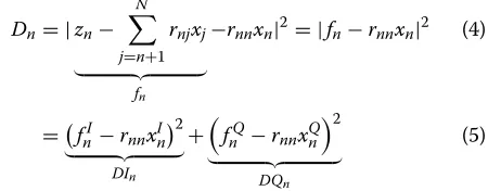
Firstly,Dnin (3) is rewritten into (4) and (5) as follows.

Dn= |zn−

In the first quarter of the constellation (in which IP and QP parts are both non-negative), we divide

the IP space into √W − 1 subdomains such as

[0,rnn), [rnn, 2rnn),. . ., [

√

W −2,∞). Each subdomain is associated with a set of ceil(√L) best values of xI_n. For example, if the modulation is 16-QAM andL =9, the IP

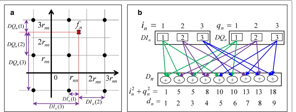
space is divided into [0,rnn), [rnn, 2rnn), and [2rnn,∞) sub-domains. The corresponding three best values ofxI_n are (1,−1, 3), (1, 3,−1), and (3, 1,−1), respectively (refer to Figure 2a). With QP space andxQn, we do similarly.

The L best child nodes per parent node in stage n

(n=N,. . ., 1) are directly specified as follows:

Step 1. Calculatefnthat is defined in (4).

Step 2. Determine the IP subdomain thatf_nIbelongs to by comparingf_nIwith values such asrnn,2rnn, . . . ,√W−2rnn. From that, theceil

√

Lbest values ofxI_nwill be known. Iff_nI<0, the signs of xI_nare reversed. Then, we calculate the

correspondingDInin (5). ThexQn andDQnare found similarly (refer to Figure 2a).

Step 3. Fromceil√Lbest values ofx_nI,DIn, andxQn, DQn, we computeLbest values ofxnandDnin (5). Let callinandqnas the index numbers of the best values ofDInandDQn, which are already in ascending order. The combination of the sumDn=DIn+DQnis arranged so that the sumi2_n+q2_nincreases. Consequently, the results ofDnare approximately in ascending order without sorting (refer to Figure 2b).

To expandLbest child nodes from a parent node, the previous works such as [5] firstly finds the center node by rounding the resultxc = fn/rnn. It then seeks forL near-est nodes to the center node. The divider is thus required. By comparing as step 2, the proposed algorithm can elimi-nate the dividerfn/rnn. Furthermore, by using (5),Lvalues ofDnare obtained fromceil(

√

(4)

Figure 2Direct expansion.(a)ComputeDIn,DQn.(b)ComputeDn. This is the illustration for case of 16-QAM,L=9. In this figure,in,qn, anddn denote the index number ofDIn,DQn, andDn, respectively.

3.2 Parent node grouping

It is important to know how much should the number of child nodes per parent node (L) be. IfL is too large, BER performance is improved. However, the decoder’s complexity is also increased. If L is too small, the BER performance may be too small to fulfill the system require-ment.

Notice that once theLbest child nodes are directly spec-ified as mentioned in Section 3.1, if L > K, there is no probability that one of the lastL−Kchild nodes of any par-ent will become the final selection. Thus, selectingL≤K is a way to reduce the complexity without trade-off of the performance.

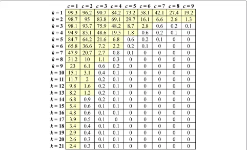
In another aspect, assume that k and care the index number of the K parent nodes (PEDn+1) and of the L child nodes (Dn) per parent node in stagen, respectively. Because values of PEDn+1are already sorted in stagen+1, the parent node that has high index k will have a large value of PEDn+1. Thus, its child nodes are expected to have low probability to be selected as one of theKsmallest (best) nodes for the next stage. To prove this analysis, we did the simulation and computed the probability (in %) in which a child node might become one of theKbest nodes. The result is shown in Figure 3. From this figure, it can be seen that the larger the indexkis, the smaller the number of child nodes may be selected.

Based on that fact, we propose a parent node grouping method as follows: TheKparent nodes are divided intoG groups. Each group hasA=K/Gparent nodes. Note that KandGshould be selected so thatKis dividable toG(i.e., mod(K,G)=0). Group 1 contains the best parent nodes, while groupGcontains the worst parent nodes. Each par-ent node of thegth (g=1, 2,. . .,G) group is expanded by Lgchild nodes so thatLG<· · ·<L1≤K.

3.3 Two-dimensional sorter

Sorting is the major bottleneck of the K-best decoder because of its high complexity. Theoretically, the sorting ofnelements requires(n2−n)/2 comparators.

In this subsection, we propose a two-dimensional (2D) sorter which has low complexity, is suitable for hard-ware resource sharing, and produces approximate result. The 2D sorter for sortingC = G_g₌₁ALgchild nodes is described as follows: we put the C child nodes into an A× B matrix, in which B = G_g₌₁Lg. Thejth row of the matrix contains all the child nodes of the jth parent of all groups. The illustration in the caseG= 3 is shown in Figure 4. The matrix operates through two processes called as row sorting and column sorting, one after the other, as follows:

• Row sorting. TheBelements in a row are sorted. The smallest value is located in the left of the row. This sorting is repeated for all rows.

• Column sorting. TheAelements in a column are sorted. The smallest value is located in the top of the column. This sorting is repeated for all columns.

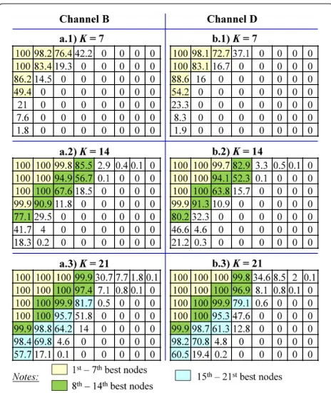
After completing the row and column sorting, the K top-left elements of the sorted matrix are expected to be the best (smallest) values and are selected. A simulation is needed in advance to correctly determine the position of the best candidates.

(5)

Figure 3Probability (in %) that a child node may be selected as one ofKbest nodes.The simulation parameters are 4×4 IEEE 802.11ac simulator, 256-QAM modulation, 148,000 data samples,K=21, andL=9. The data which haveprobability≥1% are marked by yellow color.

one determined. The figure also shows that the obtained results (in %) are slightly affected by channel type. How-ever, the influence is too small so that the position of the best nodes is not affected by channel type.

The 2D sorter is suitable for hardware resource sharing because all the rows (columns) do the same task. A circuit which sortsBelements of the 1st row in the 1st cycle can be reused to sort the 2nd, . . . ,Ath rows in the 2nd, . . . ,Ath cycles.

Figure 4Illustration of a 2D sorter.The parameters areG=3, K=21, andA=7.

4 Hardware design

4.1 Overview architecture

To determine the effectiveness of the proposed

algorithm practically, we develop a 4 × 4 2D

sorter-based K-best MIMO decoder for 802.11n and 11.ac

systems. The decoder supports five modulation

types such as BPSK, QPSK, 16-QAM, 64-QAM, and 256-QAM. After completing exhaustive simulation and considering the trade-off between BER perfor-mance and complexity, the decoder is configured as follows:

• At all stages, we selectK =21,G=3,A=K/G=7, L1=4,L2=3,L3=1,B=8, andC=56. In the case of 16-QAM, QPSK, and BPSK, which has W <K, the numbers of parent nodes of stages 3, 2, and 1 (denoted byK3,K2, andK1, respectively) are selected as follows: with 16-QAM mode,K3=14and K2=K1=21; with QPSK mode,K3=4,K2=14, andK1=21; and with BPSK mode,K3=2,K2=4, andK1=8.

• Stage 4 does not use the sorter, while stages 3 and 2 use the proposed 2D sorter with the matrix size of 7×8.

(6)

Figure 5Probability (in %) that an element of the sorted matrix becomes one of the actualKbest nodes.The simulation parameters are 802.11 ac simulator, 256-QAM, 148,000 data samples, channels B and D, 21 parent nodes,G=3,L1=4,L2=3, andL3=1.

This configuration is illustrated in Figure 6a.

PED4= |z4I−r44x4I|2

The overview hardware architecture of the decoder is

shown in Figure 6b. The ‘STAGE 4’ block computes K

best values of PED4and the correspondingx4in (6). Simi-larly, the ‘STAGE 3’ block computesKbest values of PED3 and the corresponding{x4,x3}in (8). The ‘STAGE 2’ block computes K best values of PED2and the corresponding

{x4,x3,x2}in (10). The ‘STAGE 1’ block computesCbest values of PED1 and the corresponding {x4,x3,x2,x1} in

(12). The ‘LLR’ block computes the log likelihood ratio. The ‘Multiplier-Less’ block prepares necessary data so that no multiplier will be implemented in all the above-mentioned blocks.

4.2 Hardware implementation

To achieve low complexity, in addition to utilize the pro-posed algorithm, the following implementation points are worth to be noticed.

4.2.1 GAIN-MUX-based multiplier

From (6) to (12), it can be seen that the decoder requires a large number of multipliers to compute rijxj (i = 4, 3, 2, 1;j≥ i). For example, 2√Kmultipliers are needed to compute r44xI₄ andr44xQ₄ in stage 4 (see (6)), and the multiplier costs large hardware resource.

To computerijxj(i=4, 3, 2, 1;j≥i), instead of using the multiplier, we implement GAIN and multiplexer (MUX) as be shown in Figure 7. This figure illustrates the case of multiplyingrijwithmbest values ofxj. The left figure shows the conventional method which uses m different multipliers. The right figure is our proposed GAIN-MUX-based multipliers. The input datarij firstly goes into the ‘GAIN’ block that amplifiesrij by the modulation gainD and then by the values of the constellation points such as 1, 3, 5,. . ., 15. Notice that all the possible values ofxj are {D, 3D,. . ., 15D}. The outputs of ‘GAIN’ blocks are then inputted tomMUX blocks. Each MUX is controlled by a select signal ofxj (i.e., denoted by sel_x(_jm)). If

val-ues ofx(_jm)are{D, 3D,. . ., 15D}, values ofsel_s(_jm)will be

{0, 1,. . ., 7}. Consequently, the outputs of MUX blocks are equivalent to the outputs of multipliers in the left figure. Meanwhile, hardware cost for MUX is much smaller than that for the multiplier.

The decoder needs multipliers to compute many data, such as r44xI₄, r₃₃I xI₃, andr22xI₂, while possible values of xI₄, xI₃, and xI₂ are the same. Thus, one ‘GAIN’ block can be shared among them. The ‘Multiplier-Less’ block implements this ‘GAIN’ block.

4.2.2 Resource sharing

This technique is implemented in STAGE 4, STAGE 3, STAGE 2, and STAGE 1 blocks.

The STAGE 4 block computesK best values of PED4

andx4 in (6). Based on the direct expansion method, it finds ceil √21

(7)

Figure 6Hardware design.(a)Decoder’s configuration and(b)the corresponding overview hardware architecture.

‘SIGN ABS’ block determines the sign and absolute value of|zI₄|(and|zQ₄|). The ‘CONS-LOCAT’ block specifies the subdomain in the constellation that|zI₄|(and|zQ₄|) belongs to. Based on information of the CONS-LOCAT block, the ‘DI/DQ CAL’ block computes the best values ofDI4and

DQ4, while the ‘XDE-CODE’ block finds the best values of xI₄andxQ₄.

The STAGE 3 block computes the best values of PED3 and the corresponding{x4,x3}in (8). The block diagram is shown in Figure 8c, in which ‘B1,’ ‘B2,’ and ‘B3’ respectively

(8)

a

b

c

Figure 8Block diagram of ‘STAGE 4’ and ‘STAGE 3’.(a)STAGE 4,(b)BLOCK A, and(c)STAGE 3.

perform the direct expansion for the 1st7th (i.e., group 1), 8th14th (i.e., group 2), and 15th21st (i.e., group 3) parent nodes. Because all parent nodes in the same group process similarly, they can share the same circuit. Con-sequently, the B1 block is designed to findL1 best child nodes of one parent node only. It is then reused in seven clock cycles to complete the direct expansion for seven parent nodes of group 1. The sharing factor is 7. Similarly, the B2 and B3 blocks are shared by seven times. Each B1, B2, and B3 block has the following components: ‘CALf3’ computesf3in (7), ‘BLOCK A*’ computesDI3andDQ3, and ‘SUM’ computesPED3fromPED4,DI3, andDQ3(see (8)).

After each clock cycle, B1, B2, and B3 output the best child nodes of one parent node in all groups. In other words, all elements of one row in the sort matrix (see Section 3.3) are obtained per cycle. Block ‘2D-SORT’ thus requires only a one-row-sorting circuit. This circuit is then shared to sort all seven rows in seven clock cycles. The sharing factor is 7. The hardware design of the 2D-SORT block is shown in Figure 9. The ‘ROW-2D-SORT’ block sorts eight outputs of B1, B2, and B3 per clock cycle. Only four best data are obtained. In the ‘COL-SORT’, the ‘1to7’ collects the best values from ROW-SORT in seven cycles and sorts them. The ‘1to6’ block collects the 2nd best values from ROW-SORT in seven cycles, sorts them, and obtains six best data, so on. The designs of ROW-SORT and ‘1to3’ of COL-ROW-SORT are shown in Figure 9b,c, respectively. It can be seen that the 2D-SORT needs only 36 comparators to sort 56 child nodes, which is signif-icantly reduced as compared to (562 −56)/2 = 1, 540 comparators if using the full sort.

The architectures of STAGE 2 and STAGE 1 are simi-lar to STAGE 3. The sharing factor of these blocks is 7.

However, the 2D-SORT block is not implemented in STAGE 1. Instead, the results of B1, B2, and B3 are directly passed to the LLR block.

5 BER performance comparison

The 802.11ac simulator with the following options were used in our simulation: 4×4 MIMO and transfer packet number of 5,000. Total transfer data was 2.5×106_bytes. Bandwidth was 80 MHz. Channel type was D. Forward error correction (FEC) type was binary block code (BCC).

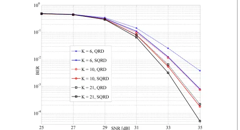
5.1 QRD versus SQRD

Figure 10 shows that using SQRD pre-processing helps to

improve BER performance by 0.6 dB, 0.8 dB (at BER =

10−3), and 1 dB (at BER = 10−2) for cases ofK = 21, K =10, andK =6, respectively, as compared to the case of using QRD.

5.2 Parent node grouping

Figure 11 shows that the BER performance is

insignificantly degraded when ‘L1-L2-L3’ is decreased from 256-256-256 (full K-best) to 9-9-9, 9-6-3, 4-4-4, and 4-3-1. Numerically, the performance degradation of L1-L2-L3 = 4-3-2 is about 0.15 dB as compared to the fullK-best (at BER = 10−3). However, when continuing to reduce the number of child nodes per parent node to L1-L2-L3 = 1-1-1, the performance degradation is about 1.2 dB, which is considerable, as compared to the full K-best.

5.3 2D sorter

(9)

a

b

c

Figure 9The design of ‘2D-SORT’ block.(a)2D-SORT,(b)ROW-SORT, and(c)1to3.

(10)

Figure 11BER of 802.11ac system: parent node grouping.G=3,K=21, 256-QAM, and SQRD were used in all cases.

Figure 12BER of 802.11ac system: 2D Sorter.K₌21,G₌3,L1=4,L2=3,L3=1, 256-QAM, and SQRD were used in all cases. The terms ‘S4

(11)

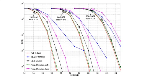
Figure 13BER of 802.11ac system: various MIMO decoder types.80 MHz, channel D, and FEC = BCC were used for all cases. For the fullK-best, K=14 in stage 4 of 16-QAM case. Otherwise,K=21. The proposed decoder is configured as Section 4.1.

case ofS4 FullSort - S32 FullSort. The amount of degrada-tion is about 0.08 dB (at BER=10−3_{). In other words, (1)} by applying the direct expansion method, the sorter can be eliminated in stage 4, and (2) the 2D sorter is an acceptable approximation of the full sorter. It can be used in trade-off with about 0.08-dB BER performance.

5.4 The proposed decoder

Figure 13 shows the BER of 4×4 MIMO 802.11ac system

when applying BLAST MMSE, LRA-MMSE, fullK-best

(soft decision), and the proposed decoder (soft and hard decisions).

From this figure, it can be seen that for all modulation types (16-QAM, 64-QAM, and 256-QAM), the proposed decoder with soft decision (green line) outperforms the BLAST MMSE (blue line) and LRA MMSE (black line), and is close to the fullK-best with soft decision (red line). Numerically, at the observation point of BER = 10−3, the proposed decoder (with soft decision) is better than BLAST MMSE by 6.7, 3.7, and 2.3 dB, respectively. It is better than LRA MMSE by 1, 0.5, and 0.02 dB, respec-tively. As compared to the fullK-best, the BER perfor-mance degradation of the proposed one is about 0.2 dB for all cases. In addition, using soft decision can improve the performance of the proposed decoder by about 2 dB as compared to the hard decision (green line versus pink line).

From this figure, we also see that the BER performance’s gap from the proposed decoder (soft decision) and the

full K-best to the LRA MMSE and the BLAST MMSE

decreases when the modulation types increase from 16-QAM to 64-16-QAM and to 256-16-QAM. That is because the modulation size increases while the K value is fixed to 21. Consequently, the BER performance of the proposed decoder and of the fullK-best is expected to be worse as the modulation size increases.

Notice that in cases of BPSK and QPSK, the proposed decoder searches all of the constellation nodes; it thus achieves the same BER as the optimal MLD does.

6 Complexity comparison

Due to the application of the direct expansion method, the number of search candidates (or visited nodes) of the pro-posed decoder is no longer affected by the constellation size. It is affected byK,Lg(g=1,. . .,G), andNonly.

Numerically, we compare the complexity of the pro-posed algorithm with the previous works in terms of total number of visited nodes (shorted as ‘total nodes’) in Table 1. All the compared algorithms are configured to

be 4×4 MIMO decoder (N = 4). The data of [3] and

[4] are obtained from their papers. Data of [5] is calcu-lated by ourselves after understanding the algorithm. In the best of our knowledge, this algorithm needs to visit √

(12)

Table 1 Total visited nodes of 4×4K-best-based MIMO decoders

Algorithm [3], 2008 [4], 2012 [5], 2013 Proposed

Modulation 256-QAM 256-QAM 64-QAM 256-QAM

Kvalue 26 26 10 21 21

Total nodes 1024 1004 189 387 189

nodes, in which RSE_num = 4 and RSE_num = 3 are

reported to be optimal for the case ofN=4,K=10, and

W =64 (64-QAM).

This table shows that

• As compared to [3] and [4], the total nodes of the proposed algorithm reduces about 8.5 times, while the gap of theKvalue is about 1.24 times.

• The total nodes of the proposed algorithm is about half of that of [5], while both have the sameK =21 and the proposed one supports higher modulation than [5] (256-QAM versus 64-QAM). In case [5] supportsK=10and the proposed supportsK=21, they have the same total nodes.

The comparison in Table 1, however, just reflects the algorithm’s complexity in terms of total nodes. The com-plexity on computing the Euclidean distance of each visited node and on sorting the nodes cannot be seen.

To compare the decoder with the previous ones thor-oughly, we designed and synthesized our decoder in ASIC. The synthesis tool was the Design Vision of Synopsys. The CMOS SAED 90 nm technology and saed90nm_minlibrary were used. The applied voltage was 1.32 V.

The ASIC synthesis results are shown and compared in Table 2. All the designs are 4×4 K-best-based MIMO

decoders. From this table, the contribution of the pro-posed decoder can be seen as follows:

High throughput. The proposed decoder achieves the highest throughput among all designs. Comparing with the most recent work in [5], the proposed decoder’s throughput is two times higher.

Low power consumption. Among all the designs, the pro-posed design consumes the least power, which is about 56 mW.

Small area. Although supporting higher modulation (i.e.,

256-QAM) and larger K (i.e., K = 21) than the most

recent work in [5], the proposed decoder occupies less hardware area. It needs 180 Kgates, which is almost half of [5]. Remember that the proposed decoder and [5] have the same number of visited nodes (see Table 1). This is the evidence for the effectiveness of the 2D sorter and computation method of the direct expansion.

High normalized hardware efficiency (NHE). The

proposed design obtains the highest NHE. It is 15.2 Mbps/Kgate, which is better than [8,11,12], and [5] by 50.7, 29.2, 8.5, and 3.6 times, respectively.

Short latency. The proposed design has the shortest latency. It is 0.07 μs.

7 Conclusions

In this paper, we have proposed an algorithm and hard-ware design of a 2D sorter-basedK-best MIMO decoder that supports up to 256-QAM. By utilizing the ideas such asdirect expansion,parent node grouping, and2D sorter, the algorithm has been proven to be less complex than the previous works, and its complexity is negligibly affected by the constellation size. A prototype hardware architecture

of the algorithm has been developed to support 4 ×

4 MIMO 802.11n and 11ac systems. Some techniques

Table 2 ASIC synthesis results of 4×4K-best-based MIMO decoders

Design [7], 2006 [6], 2006 [8], 2010 [9], 2012 [11], 2007 [12], 2010 [5], 2013 Proposed

Modulation 16-QAM 16-QAM 64-QAM 64-QAM 64-QAM (4-64)QAM 64-QAM (2-256)QAM

Kvalue 5 5 5-64 10 64 N/A 10 21

Method Real Real Real Real Complex Complex Complex Complex

Process 0.35 μm 0.25 μm 65 nm 0.13 μm 0.13 μm 0.13 μm 0.13 μm 90 nm

Hard/soft decision N/A N/A Hard Hard Soft Soft Hard Soft

fmax(MHz) 100 132 158 282 270 198 417 590

Throughput 54 424 732-100 675 100 285-431 1,000 2,700

(Mbps) 210a _{1, 178}a ₅₂₉₋₇₂a ₉₇₅a ₁₄₀a ₄₁₁₋₆₂₃a _{1, 444}a _{2, 700}a

Area (Kgate) 91 114 1,760 114 280 350 340 180

Power (mW) 626 N/A 165 135 94 57-74 1,700 56

NHEb(Mbps/Kgate) 2.33 10.3 0.3-0.04 8.5 0.52 1.18-1.79 4.26 15.2

Latency (μs) 2.4 0.4 N/A 0.6 N/A N/A 0.36 0.07

a_{Normalized throughput from}_S_{technology to 90 nm}₌_{(throughput at}_S₎_× S

90.bNormalized hardware efficiency (NHE)=

(13)

such as resource sharing, and MUX-GAIN-based

mul-tiplier have been implemented to further reduce the complexity.

The paper has shown that the proposed decoder outperforms the BLAST MMSE and LRA MMSE,

and is close to the full K-best in terms of BER

performance. The hardware design of the decoder achieves the highest throughput (2.7 Gbps), consumes the least power (56 mW), obtains the best hardware efficiency (15.2 Mbps/Kgate), and has the shortest latency (0.07 μs). This research is, thus, expected to be uti-lized not only in 802.11n/ac but also in other MIMO systems.

Our future work is to upgrade the designed decoder so that it supports from 1×1 to 8×8 MIMO cases.

Competing interests

The authors declare that they have no competing interests.

Acknowledgements

The authors would like to thank Assoc. Prof. Masayuki Kurosaki and Ms. Reina Hongyo for their help on tool licenses and hardware design. This work was partly supported by Japan Ministry of Education KAKENHI (22360156) and by VLSI Design and Education Center (VDEC), the University of Tokyo in collaboration with Synopsys.

Author details

1_{Kyushu Institute of Technology, 680-4 Kawazu Iizuka, Fukuoka 820-8502,}

Japan.2_{Radrix Co., Ltd., 680-4 Kawazu Iizuka, Fukuoka 820-8502, Japan.}

Received: 10 February 2014 Accepted: 28 May 2014 Published: 12 June 2014

References

1. TH Tran, Y Nagao, M Kurosaki, B Sai, H Ochi, ASIC implement of 600 Mbps IEEE 802.11n 4×4 MIMO wireless LAN system, inThe 14th IEEE Int. Conf. on Advan. Commu. Tech. (ICACT). Pyeongchang Korea, 19-22 Feb. 2012, pp. 360–363

2. L Azzam, E Ayanoglu, Reduction of ML decoding complexity for MIMO sphere decoding, QOSTBC, and OSTBC, inInformation Theory and Application Workshop. San Diego, CA, USA, 27 Jan - 1 Feb 2008, pp. 18–25 3. LG Barbero, JS Thompson, Fixing the complexity of the sphere decoder

for MIMO detection. IEEE Trans. Wireless Commun.7, 2131–2142 (2008) 4. X Mao, Y Cheng, L Ma, H Xiang, Step reduced K-best sphere decoding, in

Vehicular Technology Conference (VTC Fall). Quebec, Canada, 3-6 Sept 2012, pp. 1–4

5. M Mahdavi, M Shabany, Novel MIMO detection algorithm for high-order constellations in the complex domain. IEEE Trans. VLSI Syst.21, 834–847 (2013)

6. M Wenk, M Zellweger, A Burg, N Felber, W Fichtner, K-best MIMO detection VLSI architectures achieving up to 424 Mbps, inProc. Int. Symp. Circuits and Systems (ISCAS 2006). Kos Island, Greece, 21-24 May 2006, pp. 1151–1154

7. Z Guo, P Nilsson, Algorithm and implementation of the K-best sphere decoder for MIMO detection. IEEE Trans. Sel. Areas Commun.24, 491–503 (2006)

8. S Mondal, A Eltawil, CA Shen, KN Salama, Design and implementation of a sort free K-best sphere decoder. IEEE Trans. VLSI Syst.18, 1497–1501 (2010) 9. M Shabany, PG Gulak, A 675 Mb/s, 4×4 64-QAM K-best MIMO detector

in 0.13 um CMOS. IEEE Trans. VLSI Syst.20, 135–147 (2012)

10. Y Miyaoka, Y Nagao, M Kurosaki, H Ochi, RTL design of high-speed QR decomposition for MIMO decoder. IEICE Trans. Fund. Elec., Commu. Comp. Sci, 1991–1997 (A E95)

11. S Chen, T Zhang, Y Xin, Relaxed K-best MIMO signal detector design and VLSI implementation. IEEE Trans. VLSI Syst.15, 328–337 (2007) 12. C Liao, T Wang, T Chiueh, A 74.8 mW soft-output detector IC for 8×8

spatial-multiplexing MIMO communications. IEEE Trans. Solid State Circuits.45, 411–421 (2010)

doi:10.1186/1687-1499-2014-93

Cite this article as:Tranet al.:Algorithm and hardware design of a 2D sorter-basedK-best MIMO decoder.EURASIP Journal on Wireless Communications and Networking20142014:93.