Polarization analysis of a Pi2 pulsation using continuous wavelet transform
M. Kulesh1, M. Nos´e2, M. Holschneider1, and K. Yumoto3
1Institute for Mathematics, University of Potsdam, Am Neuen Palais 10, 14469 Potsdam, Germany 2Data Analysis Center for Geomagnetism and Space Magnetism, Kyoto University,
Kitashirakawa Oiwake-cho, Sakyo-ku, Kyoto 606-8502, Japan
3Space Environment Research Center, Kyushu University, 6-10-1 Hakozaki, Fukuoka 812-8581, Japan
(Received December 4, 2006; Revised May 21, 2007; Accepted May 31, 2007; Online published August 31, 2007)
In this contribution, we extend a series of previous works focused on an investigation of signal’s polarization attributes using the continuous wavelet transform, where we proposed a method to map instantaneous polarization attributes of multicomponent signals in the wavelet domain and explicitly relate these attributes with the wavelet transform coefficients of the analyzed signal. In this work, we applied our polarization method to an examination of characteristics of Pi2 pulsations. We have shown some merits of the use of the continuous wavelet transform for the Pi2 pulsations’ analysis. First, we used our polarization method for the geomagnetic field data from the MSR, KAK, GUA, SMA, BLM and LAQ observatories and showed some correlations between the polarization parameters of pulsation and the station’s position (nightside or dayside). Secondly, we considered the signal’s north components of a pair of stations and demonstrated a time-frequency variations of the phase difference between two stations during the pulsation.
Key words:Polarization attributes, multicomponent signal, wavelet transform, Pi2 pulsation.
1.
Introduction
Pi2 pulsations are defined as damped oscillations of the geomagnetic field with the period range of 40–150 s. This kind of pulsations can be observed clearly at low- and mid-latitude ground stations at substorm onset. Recent studies (Nos´eet al., 2003, 2006) have shown that low-latitude Pi2 pulsations can be found at multiple stations which are lon-gitudinally separated by a large distance of about 5–11 h of magnetic local time (MLT). These researchers found out that most of Pi2 pulsations does not have any phase dif-ferences among the stations, implying that the longitudinal wave number of pulsations (m) is close to zero. However, they also found a small number of Pi2 pulsations which have small phase differences corresponding to|m| ∼0.24– 0.48. Kosakaet al.(2002) and Hanet al.(2003) reported that the dominant frequency of mid- and low-latitude Pi2 pulsations depends on the local time. It is therefore impor-tant to examine the longitudinal dependence of low-latitude Pi2 pulsations’ characteristics (i.e. phase difference or fre-quency), since this provides information to reveal the exci-tation mechanism of Pi2 pulsations.
Fourier analysis is a traditional tool by which to analyze a time series. It has been used to determine the dominant fre-quency of a signal as well as the phase difference between two signals. However, it is difficult for Fourier analysis to detect changes of dominant frequency or phase difference within a short time, such as few wave cycles.
Frequency-dependent measurements or time-frequency analysis are particularly suitable to resolve these
time-Copyright cThe Society of Geomagnetism and Earth, Planetary and Space Sci-ences (SGEPSS); The Seismological Society of Japan; The Volcanological Society of Japan; The Geodetic Society of Japan; The Japanese Society for Planetary Sci-ences; TERRAPUB.
dependent properties. This analysis consists of an exami-nation of the frequency content variation of a signal over time. For the extended analysis of two- or three-component signals, the time-frequency representation can be incorpo-rated into the polarization analysis (Pinnegar, 2006; Diallo et al., 2006). Several methods are proposed in the literature for polarization analysis of multicomponent data. Some of these methods allow the polarization attributes to be deter-mined directly from the multicomponent signal (Morozov and Smithson, 1996; Reneet al., 1986), others are based on the analysis of the covariance matrix of multicomponent recordings and principal component analysis using the sin-gular value decomposition (Kanasewich, 1981).
In our previous work (Dialloet al., 2006), we proposed a new method of polarization analysis based on the continu-ous wavelet transform, which enables the computation of all polarization properties and, in particular, the instantaneous frequency and the instantaneous phase difference. In this paper, we apply this new method to some of Pi2 pulsation events and investigate how the phase difference of a signal is changing within a short time.
The continuous wavelet used in our approach is not crit-ical for understanding the presented results. Other meth-ods of time-frequency analysis, such as the Gabor trans-form or the S-transtrans-form, can be generally used to obtain the polarization properties. The relative performance of po-larization analysis from this different approach is primarily controlled by the frequency resolution capability. Partic-ularly, the short-time Fourier transform or the typical dy-namic spectrum can be very helpful in the analysis of ge-omagnetic pulsations in the case of the spectral resolution being important. However, the main subject in this paper is the observation of the time variations of polarization
calculate polarization properties of two-component signals in the time-frequency domain. This new method will be applied to the geomagnetic field data, and the results of this analysis will be presented in Section 4. The last section presents conclusions.
2.
Introduction to the Continuous Wavelet
Trans-form
At least two different perspectives exist for wavelet anal-ysis. The first one is the interpretation of the wavelet trans-form as a time-frequency analysis tool. The second ap-proach uses the wavelet analysis as mathematical micro-scope, and is therefore closely linked to approximation the-ory (Holschneider, 1995). Our present work focuses on the first approach of wavelet analysis.
The continuous wavelet transform of a real or complex signalS(t)∈ L2(R)with respect to a mother waveletg(t)
is the set ofL2-scalar products of all dilated and translated
wavelets with an arbitrary signal to be analyzed:
WgS(t,a)= gt,a,S = through dilationa and translationt. The symbol(.)∗ de-notes the complex conjugate. The waveletg(t)is assumed to be a function which is well localized in time and fre-quency and obeys the oscillation condition−∞+∞g(t)dt = 0.
The signalS(t)can be recovered from its wavelet trans-form as
wherem(t)is the wavelet used for the inverse wavelet trans-formMm, andωis the angular frequency. In the general case, the waveletm(t)can be different from the direct trans-form waveletg(t).
In the particular case, for the inverse wavelet transform we might choose theδ-function for the waveletm(t), which then gives us the rather simple reconstruction formula
S(t)= 1
central frequency, it can be possible to obtain the physical frequency directly by taking the inverse of the scale.
The choice of the analyzing wavelet depends on what typical oscillation modes are present in the signal. For ex-ample, to analyze rectangular oscillations, the real HAAR wavelet or a similar but symmetric FHAT wavelet is most suitable. If only one component of geomagnetic signals is analyzed, any real wavelets based on different-order deriva-tives of the Gaussian are convenient. However, the method of polarization analysis proposed in the next sections is based on a complex wavelet.
We also will need later a feature of the wavelet transform which allows us to separate the wavelet spectrum into pro-gressive and repro-gressive components,
To perform such a separation for nonprogressive wavelets, one must first calculate the Hilbert transform of the source signal, which makes the numerical procedure more
com-plex. Therefore, we use here a complex progressive
wavelet, which has zero Fourier coefficients for negative frequencies.
For example, we can consider the widely used complex Morlet wavelet consisting of a plane wave modulated by a Gaussian
g(t)=e2πi te−t2/(2σ2), g(ω)ˆ =σ√2πe−σ2(ω−2π)2/2,(4)
whereg(ω)ˆ denotes the Fourier transform of the wavelet g(t) and σ describes the variance of the wavelet. The Fourier transform of this wavelet is real-valued. Strictly speaking, the Morlet wavelet is neither progressive or re-gressive nor admissible but can be considered to be numeri-cally equivalent to a progressive or regressive wavelet when σ >5.
We also can similarly use the complex Cauchy wavelet of powerp(Fig. 1). This wavelet can be written as
Fig. 1. An example of complex Cauchy wavelet in (a) time domain and (b) frequency domain.
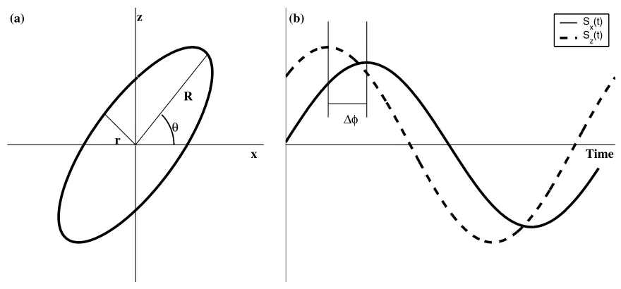
Fig. 2. Schematic representation of an ellipse with its geometric parameters: the semi-major axisR, the semi-minor axisr, the tilt angleand the phase differenceφbetweenSx(t)andSz(t). The componentsxandzare related to the north and east components of magnetic data respectively.
3.
Instantaneous Polarization Attributes in the
Wavelet Domain
Reneet al.(1986) proposed a method for multicompo-nent analysis based on complex trace analysis (CTA). This method allows the computation of instantaneous polariza-tion attributes. However, the CTA-based method operates only in the time domain, and the estimated attributes repre-sent an average over all frequencies and therefore do not provide information on their frequency dependency. To cope with these limitations inherent to time-frequency res-olution, we use here a method based on the continuous wavelet transform proposed by Dialloet al.(2006). First, we briefly introduce this method.
Our goal is to derive instantaneous polarization attributes from two signals,Snorth(t)andSeast(t), corresponding to the
north and east components of magnetic data, respectively. Using these components, we construct a complex signal
Z(t)=Snorth(t)+i Seast(t). (6)
In its full generality, an elliptically polarized rotating signalZ(t)is described by following geometric parameters (Fig. 2):
1) R: the semi-major axisR≥0,
2) r: the semi-minor axisr≥0,
3) ρ=r/R: the ellipticity ratio,ρ∈[0,1],
4) : the tilt angle, which is the angle of the semi-major axis with the horizontal axis,∈[−π/2, π/2], and 5) φ: the phase difference betweenSnorth(t)andSeast(t)
components.
The key idea to obtain instantaneous polarization at-tributes is the approximation of the complex signalZ(t)at the time pointt by a turning ellipseC(τ) on the complex plane (Fig. 2(a)). The most general turning ellipse is pa-rameterized by two complex numbers,A+andA−and two real numbersω+andω−:
C(τ)=A+eiω+τ+A−e−iω−τ.
This formula, along with geometrical considerations, yields the following relationships:
R= |A+| + |A−|, r = ||A+| − |A−||,
= 1
2arg(A +A−),
φ=arg A
++(A−)∗
A+−(A−)∗
+π
2.
prop-Fig. 3. Time-frequency spectrum of the complex synthetic signal: (a) north (solid line) and east (dotted line) components of the signal, (b) the modulus and (c) the phase of the wavelet spectrum.
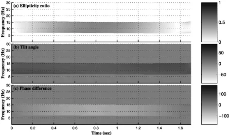
Fig. 4. Time-frequency polarization spectrum of the complex synthetic signal: (a) the ellipticity ratio, (b) the tilt angle and (c) the phase difference betweenSnorth(t)andSeast(t)components.
erty (3) of the wavelet transform allows us to represent the wavelet spectrum as a superposition of its progressive and regressive components. Let us consider the instantaneous angular frequency defined as the derivative of the com-plex spectrum’s phase:ω±(t, f)= ±∂argWg±Z(t, f)/∂t,
Then, near time instantt, each component can be repre-sented as follows:
WgZ(t+τ, f)Wg+Z(t,f)e iω+(t,f)τ
+W−
g Z(t,f)e−
which yields the time-frequency spectrum for each of the
To demonstrate these instantaneous properties, let us con-sider a synthetic example. In the next section, we will ap-ply polarization method (7) to the investigation of phase differences in the geomagnetic records; therefore, we con-sider as an example a sinusoidal waveform with a single fre-quency component, constant amplitudes, and smooth phase changes. This signal is not based on a physical model; our aim is to show the time-frequency resolution of our method with reference to the analysis of the phase difference. We define the complex synthetic signal having a small phase difference between its two components as follows:
Z(t)=Snorth(t)+i Seast(t),
Snorth(t)=Rsin(2πf0t+sin f1t),
Seast(t)=rsin(2πf0t),
where f0 = 10 Hz, R = 1.5,r = 1, and f1 = 2. This
signal is shown in Fig. 3(a).
We choose the Cauchy wavelet with parameter p = 20 (see Eq. (5)) and apply the continuous wavelet transform introduced by Eqs. (1) or (2) for the frequency range from
−30 to 30 Hz. It allows us to obtain the full wavelet spec-trumWgZ(t,f)that includes both regressiveWg−Z(t, f) and progressive Wg+Z(t,f) parts (see Eq. (3)). Both parts of the wavelet spectrum are shown in Figs. 3(b, c), whereWg+Z(t,f)corresponds to positive frequencies and W−
g Z(t, f)to negative.
The analysis of the differences between progressive and regressive parts allows us to calculate all elliptic proper-ties in the corresponding time-frequency area. For such a calculation, we use Eqs. (7) and obtain the ellipticity ra-tioρ(t,f), the tilt angle(t,f)and the phase difference φ(t, f)between the Snorth(t)and Seast(t)components as
a time-frequency spectrum for the frequency range from 0.001 to 30 Hz. However, the frequency areas where the modulus|WgZ(t, f)|of the wavelet spectrum (Fig. 3(b)) is close to zero do not contain any helpful information about the signal structure; therefore it is defensible to cut-off the elliptical parameters. For example, it can be done using this modulus and a threshold parameterεas follows:
ρ(t, f)=
Because our synthetic signal is a pure harmonic function with central frequency f0 = 10 Hz, all energy content of
this signal is concentrated in the narrow frequency band from 7 to 15 Hz, which is indicated in the pictures as narrow regions over the full time interval. To plot all polarization properties (Fig. 4), we use the threshold parameterε=0.6 that corresponds to this frequency band and causes disconti-nuities at f =7 Hz and f =15 Hz. Besides, the ellipticity ratio and the phase difference show small variations from zero to the maximum and back to zero, and the tilt angle does not have any variations. This behavior corresponds with the analytical expression of this signal.
From Fig. 3(a) we can see that the phase difference be-tween the signal components at the beginning (up to 0.4 sec) and at the end (after 1.4 sec) of record is small; there-fore, we do not see it distinctly in the signal representa-tion. However, in Fig. 4(c) we can see it very clearly be-cause of the distinction between background color that in-dicates zero phase difference and color in the frequency band f = 7...15 Hz corresponding to the signal. More-over, the color change in this frequency band indicates how the phase difference changes with time. Therefore, the pro-posed method allows us to “strengthen” the phase differ-ence using a time-frequency representation.
A positive phase difference in the right-handed coordi-nate system corresponds to right-handed polarization, and negative phase difference, to the left-handed. However, by the signal construction given by Eq. (6) we assume that the x-axis is directed to the north and the z-axis is directed to the east, which defines a left-handed coordinate system. Therefore, we can interpret the positive phase difference as left-handed polarization of the signal. The phase difference shown in Fig. 4(c) is negavite, which is typical for signals with right-handed polarisation like our synthetic signal.
4.
Application to Real Data
4.1 The 20 September 1995 eventAt 0538 UT on 20 September 1995, Pi2 pulsations were observed clearly at three different MLT sectors. At the post-midnight sector (∼0200 MLT), the low-latitude station SMA (Santa Maria, −19.5◦ geomagnetic latitude (GMLAT)) and the equatorial station BLM (Belem, 8.6◦
GMLAT) observed clear Pi2 pulsations. On the
dawn-side (∼0700 MLT), Pi2 pulsation was detected at the mid-latitude station LAQ (Laquila, 42.5◦GMLAT). Even in the afternoon sector at∼1500 MLT, Pi2 pulsations were found at low-latitude stations MSR (Moshiri, 35.4◦GMLAT) and KAK (Kakioka, 26.9◦ GMLAT) and at the equatorial sta-tion GUA (Guam, 5.1◦GMLAT). This event was reported by Nos´eet al.(2003) who suggested that the substorm was initiated at pre-midnight (2100–2300 MLT) by using high-latitude ground magnetic field data.
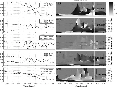
Fig. 5. Source signals and time-frequency representations of phase differences. Vertical lines bound the interval of Pi2 pulsation.
From gray-scaled images it is difficult to evaluate the ex-act numerical values of the parameters, therefore, we also showed on these images an example of the phase difference values (in degrees) at the time pointt =5.65 h and by the frequency f =0.018 Hz. However, the value of phase dif-ference in some detached points of time-frequency domain cannot be used for any physical interpretations. More suit-able for such an interpretation is the analysis of the average ofφ(t, f)either along the time or the frequency parame-ter.
One manner to reconstruct frequency-dependent quanti-ties is to average the above formulas (7) over a suitable time region in which a Pi2 has been identified in wavelet space:
φ(f)= 1
T
T2
T1
φ(τ,f)dτ.
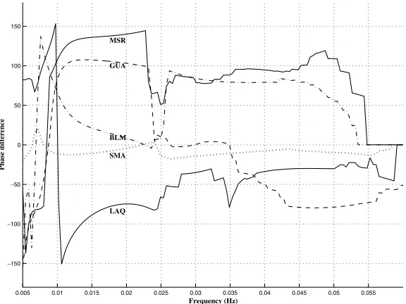
In Fig. 6, we show an example of frequency-dependent phase differences for all considered stations. SMA and BLM stations are characterized by almost zero phase differ-ence, indicating linear polarization. Previous studies have shown that Pi2 on the nightside has left-handed or linear polarization in general (Lesteret al., 1983, 1984; Lanze-rotti and Medford, 1984). Thus, our results are consistent with this. MSR and GUA, which were located around 1500 MLT, have positive phase difference in the interval 100◦– 140◦, with respect to the left-handed polarization. However,
Pi2 pulsation observed at LAQ around 0700 MLT had a neg-ative phase difference of−80◦. Nos´e (1999) reported that Pi2 pulsations have dayside polarization characteristics dif-ferent from nightside Pi2 pulsations, being right-handed be-fore local noon and changes to left-handed after local noon. Polarization of dayside Pi2 pulsations shown in Fig. 6 for LAQ station is consistent with that reported by Nos´e (1999). Figure 7 shows the ellipticity ratio and tilt angle in the time-frequency domain for Pi2 pulsations presented on the left panel of Fig. 5. The ellipticity ratios at MSR, GUA, SMA, and BLM are small, which indicates that oscillations are dominant the direction defined by tilt angle. This is consistent with results reported by Yumotoet al.(1994) and Osakiet al. (1996). Ellipticity at LAQ seems larger than that at the other four stations, implying that oscillations in the northward direction are smaller. This would be caused by the fact that LAQ was located on the dawnside, where the power spectral density of Pi2 pulsations in the northward component becomes weak (Nos´e, 1999).
Fig. 6. Frequency-dependent phase differenciesφ(f)averaged in the time interval between 5.64 h and 5.66 h.
Fig. 7. Ellipticity ratio and tilt angle in time-frequency domain for signals shown in Fig. 5.
was more variable than that other stations and was as large as ±90◦. These results suggest that the orientation of the polarization axis is different between equatorial stations and low-latitude stations.
Fig. 8. Northward components of source signals registered at different stations and time-frequency phase difference between the pair of stations.
for MSR-GUA stations), while the numerical value of this shift we can read from the right panels of the same figure. Note that the phase differences for first five examples do not depend on the time and frequency; therefore, we can inter-pret the given numerical values as mean phase differences for whole event. At the same time, two last examples, MSR-SMA and MSR-BLM show some variations of the phase difference, with the time-frequency area restricting the pul-sation, and we cannot directly interpret the numerical values as mean values.
From this figure we found that the phase difference is about−75◦for the LAQ-SMA and LAQ-BLM pairs, about
−90◦for the LAQ-MSR pair,−50◦for the LAQ-GUA pair and about 40◦ for MSR-GUA pair. There might be two possible interpretations for these phase delays: longitudinal propagation and latitudinal propagation of waves. However,
if the longitudinal propagation is the case, the observational results should be interpreted as a wave propagating from LAQ to other stations. This is not plausible. Moreover, we can see that the phase difference between MSR and GUA is about 40◦, though they are almost in the same longitude, implying the implausibility of longitudinal propagation. In-stead, these observations may be interpreted as latitudinal propagation. The latitude of LAQ is 42.5◦which is higher than that of other stations, and this may cause the phase dif-ference.
4.2 Analysis of HER-KAK stations
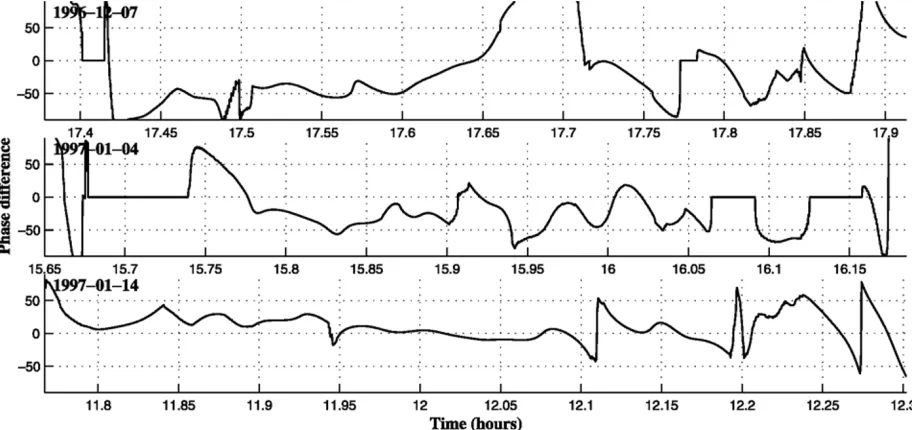
Fig-Fig. 9. North components of source signals and phase difference between HER and KAK stations for three events: 1996-12-07, 1997-01-04 and 1997-01-14.
Fig. 10. Time-dependent phase differenciesφ(t)averaged in the frequency band 0.01 and 0.015 Hz.
ure 9 shows geomagnetic field variations recorded at HER and KAK on the left panel, and the results of polarization analysis on the right panel.
Similar to the derivation of frequency-dependent at-tributes in the previous section, one may also perform an averaging of the phase difference along the parameter f (Fig. 10):
φ(t)= 1
F F2
F1
φ(t, ψ)dψ.
On the left panel for the 14 January 1997 event, we almost do not observe any phase differences between the two sta-tions during the event. Pi2 pulsasta-tions appeared in the time
interval of 11.95–12.1 h, during which oscillation peaks were coincident between HER and KAK. This character-istic is reflected in the polarization analysis shown on the right panel. There are not significant changes in color, in-dicating no clear change in phase differences. The same behavior is also observed on the bottom panel of Fig. 10, which corresponds to this event.
It is difficult to explain the phase difference found on the 7 December 1996 and 4 January 1997 events by longitudi-nal propagation of waves from the substorm onset sector. This is because the oscillation at KAK lagged behind that at HER, even though KAK was located at nighttime and HER was on the afternoon side or the duskside. Instead, the phase difference may be explained in terms of the re-flection coefficient of fast mode waves at the plasmapause. The plasmapause is not a perfect reflector for the fast mode waves, leading to leakage of the wave energy to the plasma trough (Fujitaet al., 2000, 2002). If the condition of the plasmapause is different between the nightside and the af-ternoon side, the reflection rate of the fast mode waves at the plasmapause is expected to be different and may give rise to the phase shift between two stations. The no phase difference at very beginning stage of pulsation it may be ex-plained by forcing oscillation due to the first pulse, which was propagating from the outer magnetosphere and supplies energy of the subsequent oscillations in the plasmasphere.
It may be possible to speculate that the phase change is related to the release of the magnetic energy in the magne-totail, which may be time-dependent and spatially inhomo-geneous. Further studies using data from ground stations and satellites are needed to investigate causes of the phase change in more detail.
5.
Conclusions
We propose a method for the analysis of polarization properties of geomagnetic field data using the continuous wavelet transform. The advantage of this method over pre-vious techniques like Fourier analysis is that both the time and frequency dependence of the attributes can be obtained. One important improvement by the new method is its ability to provide a means to investigate the time depen-dence of the phase difference. An important application of such information is in the determination of oscillation prop-erties of Pi2 pulsation during the event, since it provides information on the excitation mechanism of Pi2 pulsations. As shown in the presented examples, it is possible to extract all the attributes of the polarization ellipse. As a brief result of this polarization analysis, we determined that the phase difference may be somewhat sensitive to latitudes near the same MLT, and the imperfect reflecting plasma-pause might be important in determining the local phase. In general, these conclusions should need further studied in a statistical manner. However, the techniques introduced in this paper could be useful for such future studies.
References
Diallo, M. S., M. Kulesh, M. Holschneider, F. Scherbaum, and F. Adler, Characterization of polarization attributes of seismic waves using con-tinuous wavelet transforms,Geophysics,71(3), V67–V77, 2006. Fujita, S., M. Itonaga, and H. Nakata, Relationship between the Pi2
pul-sations and the localized impulsive current associated with the current disruption in the magnetosphere,Earth Planets Space,52(4), 267–281, 2000.
Fujita, S., H. Nakata, M. Itonaga, A. Yoshikawa, and T. Mizuta, A numeri-cal simulation of the Pi2 pulsations associated with the substorm current wedge,J. Geophys. Res.,107(A3), 1034, 2002.
Han, D., T. Iyemori, Y. Gao, Y. Sano, F. Yang, W. Li, and M. Nos´e, Local time dependence of the frequency of Pi2 waves simultaneously observed at 5 low-latitude stations,Earth Planets Space,55(10), 601–612, 2003. Holschneider, M.,Wavelets: an Analysis Tool, Clarendon Press, Oxford,
1995.
Kanasewich, E. R.,Time Sequence Analysis in Geophysics, University of Alberta Press, Edmonton, Alberta, 1981.
Kosaka, K., T. Iyemori, M. Nos´e, M. Bitterly, and J. Bitterly, Local time dependence of the dominant frequency of Pi2 pulsations at mid- and low-latitudes,Earth Planets Space,54(7), 771–781, 2002.
Lanzerotti, L. J. and L. V. Medford, Local night, impulsive (Pi2-type) hydromagnetic wave polarization at low latitudes,Planet. Space Sci., 32(2), 135–142, 1984.
Lester, M., W. J. Hughes, and H. J. Singer, Polarization patterns of Pi2 magnetic pulsations and the substorm current wedgee,J. Geophys. Res., 88, 7958–7966, 1983.
Lester, M., W. J. Hughes, and H. J. Singer, Longitudinal structure in Pi2 pulsations and the substorm current wedge,J. Geophys. Res.,89, 5489– 5494, 1984.
Morozov, I. B. and S. B. Smithson, Instantaneous polarization attributes and directional filtering,Geophysics,61(3), 872–881, 1996.
Nos´e, M., Automated detection of Pi2 pulsations using wavelet analysis: 2. An application for dayside Pi2 pulsation study,Earth Planets Space, 51(1), 23–32, 1999.
Nos´e, M., K. Takahashi, T. Uozumi, K. Yumoto, Y. Miyoshi, A. Morioka, D. K. Milling, P. R. Sutcliffe, H. Matsumoto, T. Goka, and H. Nakata, Multipoint observations of a Pi2 pulsation on morningside: The 20 September 1995 event,J. Geophys. Res.,108(A5), 1219, 2003. Nos´e, M., K. Liou, and P. R. Sutcliffe, Longitudinal dependence of
char-acteristics of low-latitude Pi2 pulsations observed at Kakioka and Her-manus,Earth Planets Space,58(6), 775–783, 2006.
Osaki, H., K. Yumoto, K. Fukao, K. Shiokawa, F. W. Menk, B. J. Fraser, and the 210◦MM Magnetic Observation Group, Characteristics of low-latitude Pi2 pulsations along the 210◦magnetic meridian,J. Geomag. Geoelectr.,48, 1421–1430, 1996.
Pinnegar, C. R., Polarization analysis and polarization filtering of three-component signals with the time-frequency S transform,Geophys. J. Int.,165(2), 596–606, 2006.
Rene, R. M., J. L. Fitter, P. M. Forsyth, K. Y. Kim, D. J. Murray, J. K. Walters, and J. D. Westerman, Multicomponent seismic studies using complex trace analysis,Geophysics,51(6), 1235–1251, 1986. Yumoto, K., H. Osaki, K. Fukao, K. Shiokawa, Y. Tanaka, S. I. Solovyev,
G. Krymskij, E. F. Vershinin, V. F. Osinin, and the 210◦MM Magnetic Oservation Group, Correlation of high- and low-latitude Pi2 magnetic pulsations observed at 210◦magnetic merdian chain stations,J. Geo-mag. Geoelectr.,46, 925–935, 1994.