Menzies Building
Monash University Wellington Road
CLAYTON Vic 3168 AUSTRALIA
Telephone:
from overseas:
(03) 905 2398, (03) 905 5112
61 3 905 2398 or
61 3 905 5112
Fax numbers:
from overseas:
(03) 905 2426, (03)905 5486
61 3 905 2426 or 61 3 905 5486
[email protected]
S
OLVING
A
PPLIED
G
ENERAL
EQUILIBRIUM
MODELS
REPRESENTED
AS A
M
IXTURE OF
L
INEARIZED AND
L
EVELS
E
QUATIONS
by
W. Jill H
ARRISON
Monash University
K.R. PEARSON
Monash University and
La Trobe University
Alan A. P
OWELL
Monash University
and
E. John SMALL
Australian Bureau of Agricultural
and Resource Economics
Preliminary Working Paper No. IP-61 September 1993
ISSN 1 031 9034
ISBN 0 642 10297 X
C
ENTRE
of
P
OLICY
S
TUDIES
and
the
I
MPACT
i
ii
1.
Introduction
1
2.
Stylized Johansen
2
3.
Miniature ORANI(MO)
3
4.
AIDADS: An implicit functional form
6
5.
ORANI-F
13
5.1
A mixed levels/linear representation of
ORANI-F
13
5.2
Comparison with the linear version
16
5.3
Comparative simulation performance
17
6.
Conclusion
19
References
20
TABLES AND FIGURES
Table 2.1
Levels and Linearized Equations of the
Stylized Johansen Model
3
Table 3.1
TABLO Input File for Equations in Consumer
Demand Block of MO
7
Table 4.1
TABLO Input File for a Linearized Implementation
of AIDADS
11
Table 4.2
TABLO Input File for a Levels Implementation of
AIDADS
12
Table 5.1
Comparing Linear and Mixed Implementations
of ORANI-F
18
Figure 4.1 Accumulation of the differential du in the utility
level in the solution of the AIDADS consumer
demand system
9
Figure 5.1 Typical TABLO statements from the data and
initial solution section
14
Figure 5.2 CES nest for aggregation of labour across
occupations written mainly as linearized
equations
15
Figure 5.3 CES nest for aggregation of labour across
AS
A M
IXTURE OF
L
INEARIZED AND
L
EVELS
E
QUATIONS
*by
W. Jill HARRISON K. R. PEARSON AlanA. POWELL
Monash University Monash University and La TrobeUniversity Monash University
and
John SMALL
Australian Bureau of Agricultural and Resource Economics
1. Introduction
In the past there has been a strong link between the presentation of a model's equations and the method used to solve it. Those using extensions of Johansen's (1960) linearization approach to solve a model have tended to emphasize its linearized equations in presentations of its structural form and in discussions of the economics driving its simulation results. Model builders committed to non-linear solution algorithms that do not explicitly non-linearize as a first step, on the other hand, have been less inclined to discuss structure or results in terms of linearized equations.
In a recent paper, Hertel, Horridge and Pearson (1992) argue that the apparent gulf between the North American (levels) and the Norwegian/Australian (linearizing) schools of AGE model builders is more apparent than real. The solution method, although an important part of model building practice, is in principle an issue totally divorced from the economics incorporated within a model. Differing approaches to solving any given model should, and do, yield identical solutions with identical economic interpretations.
Thus there is no compelling link between the way in which the model is presented and the manner of its solution. That said, one can nevertheless see why those who linearize for solution purposes would be more inclined also to present their work in terms of linearized equations. And because of the ever-present risk of error in implementation, one could argue that, other things equal, it is better for model builders to present the structure of their model in a form that is as close as possible to its actual computer implementation.
If the latter dictum is accepted, then, in a world in which solution software has required model builders to opt either for linearized equations (
G
EMPACK)
or for levels representations (GAMS or MPS/GE)1, it is natural that the apparent gulf between the two schools of modellers should have arisen. Current software developments, however, will obviate the necessity for model builders to choose between linearized and levels equations: the recent Release 5.0 ofG
EMPACK(Pearson and Harrison, 1993a) accepts equation systems represented in either form, or as a mixture of both. This implies that adherents of both schools have a new freedom in the formulation and presentation of models and results. The choice now can be made independently of considerations concerning solution procedures — transparency and/or convenience become the dominant considerations.
* Grant number A79030343 from the Australian Research Council has substantially assisted this work.
After brief preliminaries concerning
G
EMPACK,
the practicality and desirability of solving models presented as mixtures of levels and linearized equations are illustrated in sections 2, 3, 4 and 5. These deal with a tiny teaching model (Stylized Johansen), a somewhat larger miniature model (MO), a system of demand equations lacking an explicit closed-form levels representation (AIDADS) and the standard forecasting version of the ORANI model (ORANI-F) respectively. A summary and concluding perspective are offered in section 6.Preliminaries concerning GEMPACK and TABLO Input Files
GEMPACK is a suite of general-purpose economic modelling software. Economists who develop models can implement them using GEMPACK by writing the equations and formulae of the model in a form that is essentially the same as ordinary algebraic notation. The model is input to the computer as a text file known as a TABLO Input file (because TABLO is the program which processes the file).
In the following sections of the paper, several small TABLO Input files are given as examples because the input is easily understood and serves as complete documentation both for the computer and, with added comments and labelling, for the modeller.2
In early versions of GEMPACK, the equations in the TABLO Input file had to be written as linear equations in terms of the changes or percentage changes of the model's variables. However in the most recent version, Release 5.0 of GEMPACK, equations can also be written in the TABLO Input file as non-linear levels equations. Automatic linearization is carried out within GEMPACK to convert the non-linear equations to the associated linearized equations. TABLO Input files can contain just linearized equations, or just levels equations, or a mixture of these.
In all cases, simulation results report changes or percentage changes in the model variables. (More information about the way
G
EMPACK solves models can be found in sections 1–3 and 6 of Horridge et al., 1993.)2. Stylized Johansen
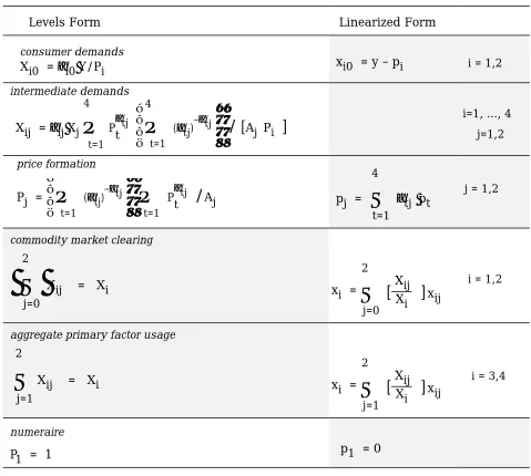
The Stylized Johansen Model (STJ) (Dixon, Parmenter, Powell and Wilcoxen, 1992, Ch. 3) is a teaching device used to introduce students to the most fundamental ideas involved in applied general equilibrium modelling. As will be apparent from Table 2.1, the first three blocks of equations are identically linear in the logarithms; consequently it is natural to discuss the economics of these equations in terms of the linearized version shown in the second column of the table. The market clearing and accounting identities shown in the next two blocks of equations, however, are much more naturally (and transparently) presented in the levels version (shown in the first column).
A GEMPACK TABLO Input file for STJ written entirely in the linearized version is given in Codsi and Pearson (1988). A TABLO Input file for the mixed version indicated by the shaded blocks in Table 2.1 is available on request from the authors.
Table 2.1
Levels and Linearized Equations of the Stylized Johansen Model*
Levels Form Linearized Form
consumer demands
Xi0 = αi0Y/Pi xi0 = y – pi i = 1,2
intermediate demands
Xij = αijXj
Π
t=1 4
Pαtj t
Π
t=1 4(αtj)–αtj
/
[
Aj Pi ]i=1, ..., 4 j=1,2
price formation
Pj =
Π
t=1 4(αtj)–αtj
Π
t=1 4
Pαtj
t
/
Aj pj =Σ
t=1 4αtj pt j = 1,2
commodity market clearing
Σ
j=0 2
Xij = Xi x
i =
Σ
j=0 2
[
Xij Xi]
xiji = 1,2
aggregate primary factor usage
Σ
j=1 2
Xij = Xi x
i =
Σ
j=1 2[ XXij
i
]
xiji = 3,4
numeraire
P1 = 1 p1 = 0
* Upper-case Roman letters represent the levels of the variables; lower-case Roman letters are the corresponding percentage changes (which are the variables of the linearized version shown in the second column). The letters P and X denote prices and quantities respectively, while the symbols A and α denote parameters. Subscripts 1 and 2 refer to the (single) commodities produced by industries 1 and 2 (subscript i), or to the industries themselves (subscript j); i = 3 refers to labour while i = 4 refers to the model's one (mobile-between-industries) type of capital; subscript j = 0 identifies consumption. Because the first three equation blocks are identically linear in the logarithms they are natural candidates for presentation and explanation of the model.
3. Miniature ORANI (MO)
The production and utility trees in MO are nested. Whilst the algebra used to derive consumers' and producers' demand functions is probably best handled in the levels, once derived their presentation becomes a matter of choice. However, in our view the most transparent explanation of the economics underlying the demand functions would be presented as a mixture of levels and linearized equations.
We illustrate this below by considering in detail the consumer demand system in MO. Industry inputs and outputs (see section 5.2 of Dixon et al., 1982) follow a similar pattern.
Consider the demands by households for each of the model's four commodities:
• domestically produced commodity 1 (household demand = X(11)3 ) • imported commodity 1 (household demand = X(12)3 )
• domestically produced commodity 2 (household demand = X(21)3 ) • imported commodity 2 (household demand = X(22)3 )
The upper nest of the utility function is Leontief in two effective commodity aggregates, X(1.)3 and X(2.)3 :
(3.1) U = Min
{
X(A(1.)31.)3 ,
X(2.)3
A(2.)3
}
, (i = 1, 2)
where the As are parameters. The variables X (1.)3 and X(2.)3 are Armington
aggregates over the domestic and the foreign sourced commodities 1 and 2 respectively. The Armington elasticity in each case is unity; hence the aggregator functions producing X(1.)3 and X(2.)3 have Cobb-Douglas form:
(3.2) X(i.)3 =
Π
s=1 2
Xα(is)3
(is)3 . (α(i1)3 + α(i2)3 = 1) (i = 1, 2)
The representative consumer's budget constraint is:
(3.3)
Σ
i=1 2
Σ
s=1 2
P(is) X(is)3 = C .
Given the non-analytic nature of (3.1) and strictly positive prices, the necessary conditions for maximization of U subject to the budget constraint lead to:
(3.4)
(
X(A(i.)3i.)3
) = R
(i = 1,2)(3.5) X(is)3 = α(is)3 X(i.)3
P(ir) P(is)
α(ir)3
/
αi∗ (s _ r; r, s = 1, 2; i = 1, 2)in which
(3.6) αi ∗ = (
α
(i1)3)α(i1)3 (α
(i2)3)α(i2)3 . (i = 1, 2)For ease of presentation it is probably optimal to define price indexes for the
effective goods; these are just the unit cost functions dual to the second-level demand functions (3.5)3:
(3.7) P(i.)3 = α1
i*
Π
s=1 2Pα(is)3
(is) =
Π
s=1 2(
αP(is)(is)3
)
α(is)3
. (i = 1, 2)
If we multiply (3.5) by P(is) and add over domestic and imported sources, after rearrangement, in the light of (3.7) we obtain:
(3.8) P(i.)3 X(i.)3 =
Σ
s=1 2
P(is) X(is)3 . (i = 1, 2)
Using (3.8) and (3.4) we see that (3.3) can be rewritten:
(3.9) C =
Σ
i=1 2
P(i.)3 X(i.)3
The consumer demand sub-system can be solved to determine the X(is)3 (i, s=1, 2) and R by using equations (3.7), then (3.4) and (3.9) jointly4, followed by (3.5).
Since (3.5) and (3.7) are linear in the logarithms, they might well be presented algebraically as:
(3.5*) x(is)3 = x(i.)3 + α(ir)3 {p(ir) – p(is) } (s ≠ r; r, s = 1, 2; i = 1, 2)
3 Note that if the base-period data is calibrated so that the P(is) (i,s =1, 2) are all unity,
then base-period values of the P(i.)3 (i =1, 2) will not have unit value.
4 One could use (3.4) to substitute [X(1.)3
A(1.)3 A(2.)3 ] for X(2.)3 in (3.9), and solve for X(1.)3
and
(3.7**) p(i.)3 =
Σ
s=1 2
α(is)3 p(is) . (1 = 1, 2)
respectively, where the lower-case Roman letters are percentage changes. Using (3.7**) and the fact that the α(is)3 add over sources s to unity for each i, (3.5*) may be rewritten:
(3.5**) x(is)3 = x(i.)3 – {p(is) – p(i.)3 ) (s = 1, 2; i = 1, 2)
The four equation blocks in shaded boxes would seem to be a sensible selection both for presentation and for solution. The first two correspond to the Leontief function and to an accounting identity respectively. Since equations with either parentage are linear in the levels, both are obvious candidates for levels presentation. The second two equation blocks, having Cobb-Douglas parentage, are linear in the logarithms, and hence are optimally displayed in linearized form. Coding of the mixed representation in the TABLO facility of GEMPACK is shown in Table 3.1.
Similar considerations apply to the representation of the nests determining industry inputs and outputs in MO (see section 5.2 of Dixon et al., 1982); these are also most naturally and informatively shown as a mixture of levels and linearized equations. The complete mixed levels/linearized TABLO Input file for MO can be obtained from the authors.
4. AIDADS: An implicit functional form
The AIDADS consumer demand system (Rimmer and Powell, 1992a&b) is an example of what Cooper and McLaren (1992b) have termed an 'effectively globally regular functional form'. Effective global regularity implies that interior tangency solutions of the consumer's allocation problem can be guaranteed for all points in the prices–expenditure space for which total spending power exceeds some lower bound (think: 'subsistence'). Relative to its parent, Stone's Linear Expenditure System (LES), AIDADS has the advantage of very flexible Engel responses. Whilst in the LES marginal budget shares are globally constant, in AIDADS they are not-necessarily-monotonic functions of total expenditure — for more details, see Rimmer and Powell (1992a).
Table 3.1
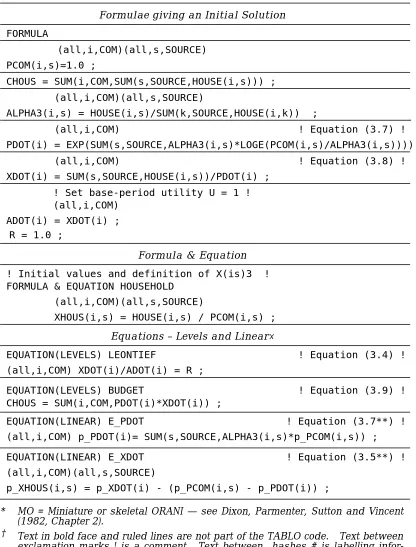
TABLO Input File for Equations in Consumer Demand Block of MO*†
Declaration of Defaults
VARIABLE(DEFAULT=LEVELS) ; FORMULA(DEFAULT=INITIAL) ;
Declarations of Sets
SET COM # commodities # SIZE 2 ;
SET SOURCE # source of commodities # (domestic, imported) ;
Declaration of Database File
FILE basedata # the file containing all base data # ;
Declarations of Variables
VARIABLE
(all,i,COM)(all,s,SOURCE)
XHOUS(i,s) # real consumption of i from source s - X(is)3 # ; CHOUS # nominal total household consumption - C # ; (all,i,COM)(all,s,SOURCE)
PCOM(i,s)
# price (local $) of commodity i from source s - P(is) # ; (all,i,COM)
PDOT(i) #Unit cost index for Armington aggregate i - P(i.)3 # ; (all,i,COM)
XDOT(i) # Armington aggregate over sources of commod.i - X(i.)3 #; (all,i,COM)(all,s,SOURCE)
HOUSE(i,s)
#nominal cons'n of commod. i from source s - P(is).X(is)3 # ; R # Consumption mix ratio (outer nest)# ;
Declarations of Parameters
COEFFICIENT(PARAMETER) (all,i,COM)(all,s,SOURCE) ALPHA3(i,s)
! share of good (is) in household's total expenditure on effective COEFFICIENT(PARAMETER) (all,i,COM) ADOT(i)
! Leontief utility coefficient - A(i.)3 !;
Read Statements
READ (all,i,COM) HOUSE(i,"domestic")
FROM FILE basedata HEADER "DOMH" ; READ (all,i,COM) HOUSE(i,"imported")
FROM FILE basedata HEADER "IMPH" ;
Table 3.1 (continued)
Formulae giving an Initial Solution
FORMULA
(all,i,COM)(all,s,SOURCE) PCOM(i,s)=1.0 ;
CHOUS = SUM(i,COM,SUM(s,SOURCE,HOUSE(i,s))) ; (all,i,COM)(all,s,SOURCE)
ALPHA3(i,s) = HOUSE(i,s)/SUM(k,SOURCE,HOUSE(i,k)) ;
(all,i,COM) ! Equation (3.7) ! PDOT(i) = EXP(SUM(s,SOURCE,ALPHA3(i,s)*LOGE(PCOM(i,s)/ALPHA3(i,s)))); (all,i,COM) ! Equation (3.8) ! XDOT(i) = SUM(s,SOURCE,HOUSE(i,s))/PDOT(i) ;
! Set base-period utility U = 1 ! (all,i,COM)
ADOT(i) = XDOT(i) ; R = 1.0 ;
Formula & Equation
! Initial values and definition of X(is)3 ! FORMULA & EQUATION HOUSEHOLD
(all,i,COM)(all,s,SOURCE)
XHOUS(i,s) = HOUSE(i,s) / PCOM(i,s) ;
Equations – Levels and Linear×
EQUATION(LEVELS) LEONTIEF ! Equation (3.4) ! (all,i,COM) XDOT(i)/ADOT(i) = R ;
EQUATION(LEVELS) BUDGET ! Equation (3.9) ! CHOUS = SUM(i,COM,PDOT(i)*XDOT(i)) ;
EQUATION(LINEAR) E_PDOT ! Equation (3.7**) ! (all,i,COM) p_PDOT(i)= SUM(s,SOURCE,ALPHA3(i,s)*p_PCOM(i,s)) ; EQUATION(LINEAR) E_XDOT ! Equation (3.5**) ! (all,i,COM)(all,s,SOURCE)
p_XHOUS(i,s) = p_XDOT(i) - (p_PCOM(i,s) - p_PDOT(i)) ;
* MO = Miniature or skeletal ORANI — see Dixon, Parmenter, Sutton and Vincent (1982, Chapter 2).
† Text in bold face and ruled lines are not part of the TABLO code. Text between
exclamation marks ! is a comment. Text between hashes # is labelling infor-mation which appears on simulation results.
Compute
Compute
C
jt= –
pjt (M – pt t′ γ )
eu 1 + e
Σ
i=1 n
ln (xit γi) –
1
–1 t
t –
φ
itCompute
=
[
α
i+
β
ie
u
t)]
[1 +
e
u
t]
x
jt=
γ
j+
p
φ
jtjt
(M
t– p
′
tγ
)
Compute
Compute
u
t+1= (u
t+
)
du
t=
Σ
j=1 n
Cjt(u ) (At jt+1 – A ) jt φjt(u )t
In multi-step
solutions,
uptdate u
tdu
tExit at 1st round in
Johansen one-step
computation
(βi - φit)
S tart
Set u = initial value, u
t
A
B
C
D
E
Compute
Compute
C
jt= –
pjt (M – pt t′ γ )
eu 1 + e
Σ
i=1 n
ln (xit γi) –
–1 t
t –
φ
itCompute
=
[
α
i+
β
ie
u
t)]
[1 +
e
u
t]
x
jt=
γ
j+
p
φ
jtjt
(M
t– p
′
tγ
)
Compute
Compute
u
t+1= (u
t+
)
du
t=
Σ
j=1 n
Cjt(u ) (At jt+1 – A ) jt φjt(u )t
In multi-step
solutions,
uptdate u
tdu
tExit at 1st round in
Johansen one-step
computation
(βi - φit)
S tart
Set u = initial value, u
tA
B
C
D
E
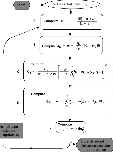
Figure 4.1 Accumulation of the differential du in the utility level in the solution of the AIDADS consumer demand system (adapted from Rimmer and Powell, 1992b)
the cost (at current prices) of the discretionary purchase of i to the cost of all discretionary purchases:
(4.1) φi (u) ≡
pi(xi – γi)
M – p'γ =
αi + βi
e
u1 +
e
u . (i = 1, 2, ..., n)Above the notation is as follows: the αi , βi and γi are the system's parameters; u is the utility level of the representative household; pi and xi are the price and quantity of i consumed, and M is total nominal spending. The vectors p and γ contain the prices pi and subsistence parameters γi respectively.
The implicit utility function can be written in terms of the φi as follows:
(4.2)
Σ
i=1 n
φi (u) ln
(
xi – γiA
e
u)
= 1,where A is a parameter.
The AIDADS demand system is a simple rearrangement of (4.1):
(4.3) xi = γi + φi (u)
pi
(
M – p'γ)
(i = 1, 2, ..., n)(4.4) = γi + φi (u) Ai , (i = 1, 2, ..., n)
where
(4.5) Ai =
(
M – p'γ)/
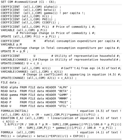
pi . (i = 1, 2, ..., n)Table 4.1
TABLO Input File for a Linearized Implementation of AIDADS
SET COM #commodities# (C1 - C6); COEFFICIENT (all,i,COM) alpha(i) ; COEFFICIENT (all,i,COM) beta(i) ;
COEFFICIENT (all,i,COM) gamma(i) ! per capita !; COEFFICIENT (all,i,COM) X(i) ;
COEFFICIENT (all,i,COM) PHI(i) ; COEFFICIENT (all,i,COM) CCOEF(i) ;
COEFFICIENT (all,i,COM) P(i) # Price of commodity i #; VARIABLE (all,i,COM) p_P(i)
# Percentage change in Price of commodity i #; UPDATE (all,i,COM) P(i) = p_P(i) ;
COEFFICIENT M #Total consumption expenditure per capita #; VARIABLE p_M
#Percentage change in Total consumption expenditure per capita #; UPDATE M = p_M ;
COEFFICIENT U # Utility of representative household #; VARIABLE(CHANGE)c_U#Change in Utility of representative household#; UPDATE(CHANGE) U = c_U ;
COEFFICIENT (all,i,COM) AJ(i) #Coeff'tAifrom eqn (4.5)oftext#; VARIABLE(CHANGE) (all,i,COM) c_AJ(i)
# Change in coefficient Ai appearing in equation (4.5) #; UPDATE(CHANGE) (all,i,COM) AJ(i) = c_AJ(i) ;
FILE data ;
READ alpha FROM FILE data HEADER "ALPH" ; READ beta FROM FILE data HEADER "BETA" ; READ gamma FROM FILE data HEADER "GAMM" ; READ M FROM FILE data HEADER "MMMM" ; READ P FROM FILE data HEADER "PRCE" ; READ U FROM FILE data HEADER "UTIL" ;
FORMULA(INITIAL) ! equation (4.5) of text ! (all,i,COM) AJ(i) = (M - sum(j,COM,P(j)*gamma(j)))/P(i) ;
EQUATION E_AJ (all,i,COM) ! linearization of equation (4.5) of text ! c_AJ(i) =
1.0/P(i)*[M / 100.0 * p_M - SUM(j,COM,gamma(j)*P(j)/100.0 * p_P(j))] - [M - SUM(j,COM,P(j) * gamma(j))]/P(i) / 100.0 * p_P(i) ; FORMULA (all,i,COM) ! equation (4.1) of text ! PHI(i) = (alpha(i) + beta(i)*EXP(U))/(1 + EXP(U)) ;
Table 4.1 (continued)
FORMULA (all,i,COM) ! equation (4.3) of text ! X(i) = gamma(i) + PHI(i)*AJ(i);
DISPLAY P ; X ; M ; U ; PHI ;
! coefficient displayed in panel C of Figure 4.1 ! FORMULA (all,i,COM) CCOEF(i) = -1/AJ(i)/
(EXP(U)/(1+EXP(U))*SUM(j,COM,(beta(j)-PHI(j))*LOGE(PHI(j)*AJ(j)))-1); EQUATION E_U ! equation displayed in panel D of Figure 4.1 ! c_U = SUM(i,COM,CCOEF(i)*PHI(i)*c_AJ(i)) ;
Table 4.2
TABLO Input File for a Levels Implementation of AIDADS
SET COM #commodities# (C1 - C6); COEFFICIENT(DEFAULT = PARAMETER) ; VARIABLE(DEFAULT = LEVELS) ;
EQUATION(DEFAULT = LEVELS) ; COEFFICIENT
(all,i,COM) alpha(i) ; (all,i,COM) beta(i) ; (all,i,COM) gamma(i) ;
LNA ; !Natural log of parameter A in equation (4.2)! VARIABLE
(all,i,COM) X(i) # Consumption of i per capita #; (all,i,COM) P(i) # Price of commodity i #;
M # Total consumption expenditure per capita #; (all,i,COM) PHI(i) # Function of utility #;
VARIABLE(CHANGE)
U # Utility of representative household #; FILE data ;
READ alpha FROM FILE data HEADER "ALPH" ; READ beta FROM FILE data HEADER "BETA" ; READ gamma FROM FILE data HEADER "GAMM" ; READ P FROM FILE data HEADER "PRCE" ; READ U FROM FILE data HEADER "UTIL" ; READ M FROM FILE data HEADER "MMMM" ;
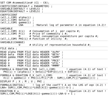
FORMULA & EQUATION E_PHI (all,i,COM) ! equation (4.1) of text ! PHI(i) = (alpha(i) + beta(i)*EXP(U))/(1 + EXP(U)) ;
FORMULA & EQUATION E_X (all,i,COM) ! equation (4.3) of text ! X(i) = gamma(i) + PHI(i)/P(i)*(M - SUM(j,COM,P(j)*gamma(j))) ; DISPLAY P ; X ; M ; U ; PHI ;
FORMULA(INITIAL) ! log of the coeff't A on the LHS of eqn (4.2) ! LNA= SUM(i,COM,PHI(i)*LOGE(X(I)-gamma(i)))-U-1 ;
5. ORANI-F
The previous sections have considered small pedagogical models (Stylized Johansen and Miniature ORANI) and the consumer demand system (AIDADS) of a larger model. In this section we report our experience with a mixed levels/linear representation of a full-scale model, namely ORANI-F. This model has been used since the mid 1980s for policy analysis and forecasting of the Australian economy.
The particular version we refer to here is documented in Horridge, Parmenter and Pearson (1993), hereafter referred to as HPP, which describes the theory in detail and analyses some typical simulation results. The implementation described in HPP is a polished, efficient, linear representation. The TABLO Input file, which contains the full set of linearized equations, is given in full in HPP. The theory is described there in various subsections, each of which shows the relevant excerpt from the TABLO Input file. We cross reference some of these excerpts in the discussion below.
The model described in HPP recognises 23 commodities, 22 sectors and 2 occupations, but the representation of the model would change only slightly for the full-sized ORANI-F (114 commodities, 112 sectors and 8 or more occupations) often used in policy simulations (see, for example, Parmenter, 1988).
To check out the desirability of using mixed levels/linear representations, we decided to implement a mixed version of ORANI-F. The basic idea behind this representation was to use levels equations where this seemed natural and easy, and to use linearized equations where that seemed more natural or easier. As expected, this meant that the various accounting identities were included in levels form while the various behavioural equations were included in linear form. Details are given in section 5.1.
The data base used is identical to that for the linear representation; it consists of input-output tables reflecting dollar values of activities and the various parameter values. (See section 4.2 of HPP for more details.)
We describe the mixed version in section 5.1, compare it to the linearized version in HPP in section 5.2, and report in section 5.3 some of our experiences in working with it.
5.1 A mixed levels/linear representation of ORANI-F
In this section we describe the main components of the TABLO Input file ORANIFM.TAB for our mixed implementation of ORANI-F. The complete file can be obtained by writing to one of the authors.
The TABLO Input file can be divided into four sections which respectively:
(1) set up the initial solution from the model's data base, (2) describe the behaviour of producers and consumers
via nested production and utility functions,
(3) specify the price system and define various price indices,
Data and initial solution section
The input-output flows (or dollar values) are read in from the data base, which includes detail about whether the flow is used for intermediate use, investment, household use, export, other demands or inventories. This data also includes flows of margins quantities, commodity taxes and tariff revenue.
Included in this section are several calculations of totals. For example, for each occupation type, the total employment of labour and its total dollar value are calculated by adding across the use of this occupation type in all industries.
G
EMPACK needs to be able to calculate the values of many of the levels variables at the initial equilibrium.5 Initial solutions for the different dollar values variables are either as read from the data base or as calculated (typically as totals, as indicated above). Initial basic prices are set to 1 and then the initial solution for the relevant quantities X are calculated via X = V/P where V is the relevant dollar value and P the associated price.The statements in Figure 5.1 illustrate the statements in this section of the TABLO Input file.6
SET IND # Industries # (I1-I22);
SET OCC # Occupation Types # (skilled, unskilled); VARIABLE (DEFAULT=LEVELS);
VARIABLE (All,i,IND)(All,o,OCC) X1LAB(i,o) #Employment#;
VARIABLE (All,i,IND) (All,o,OCC) V1LAB(i,o) #Wage bill matrix#; VARIABLE (All,o,OCC) X1LAB_I(o) #Employment by occupation#; VARIABLE (All,o,OCC) V1LAB_I(o) #Total wages, occupation o#; VARIABLE (All,i,IND)(All,o,OCC) P1LAB(i,o) #Wage#;
READ V1LAB From File MDATA Header "1LAB";
FORMULA (INITIAL) (All,i,IND) (All,o,OCC) P1LAB(i,o) = 1; FORMULA & EQUATION S_X1LAB
(All,i,IND) (All,o,OCC) X1LAB(i,o) = V1LAB(i,o)/P1LAB(i,o); FORMULA & EQUATION S_V1LAB_1
(All,o,OCC) V1LAB_I(o) = SUM(i,IND,V1LAB(i,o)); FORMULA & EQUATION E_X1LAB_I
(All,o,OCC) X1LAB_I(o) = SUM(i,lab, X1LAB(i,o));
Figure 5.1 Typical TABLO statements from the data and initial solution section
Behavioural equations section
The next section of the TABLO Input file contains the behavioural equations to determine the composition of composite commodities and the primary factor aggregate. CES nests are used for occupational composition of labour demand, for
5 Specifically, it needs to know the initial values of all levels variables occurring in the linearized equations (either those already explicit in the TABLO Input file or those produced by TABLO when it linearizes the levels equations in the TABLO Input file).
primary factor proportions, for import/domestic composition of intermediate demands and for investment demands, while a Leontief function is used for the top level of industry input demands and also investment. A CET function is used for supplies of commodities by industries.
This section is more easily handled by using linearized equations since the percentage changes in the composite quantities can be found without evaluating the associated levels values of the composite. This avoids the cumbersome calibration process which would be necessary if we had used the levels versions of these equations.
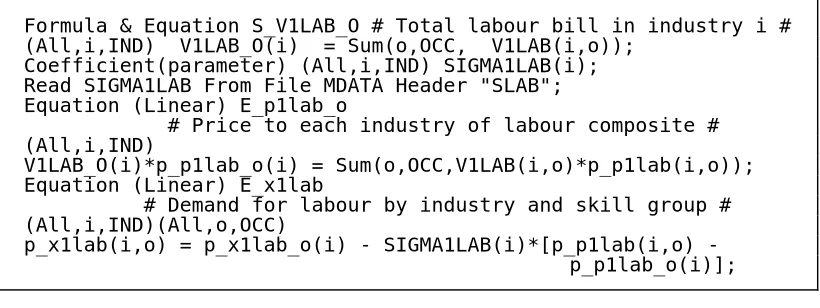
An example of TABLO input for a CES nest from the mixed ORANI-F model is given in Figure 5.2. This is Excerpt 15 of the TABLO Input file which describes the occupational composition of labour demand. The problem is, for each industry i, to select the least-cost occupational mix of labour; i.e., in TABLO-like notation,7 to minimize
(5.1.1) Sum(o,OCC, P1LAB(i,o)*X1LAB(i,o) )
such that
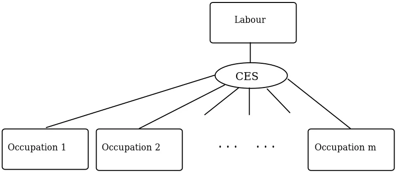
(5.1.2) X1LAB_O(i) = CES( All,o,OCC: X1LAB(i,o)).
The production structure corresponding to (5.1.2) is shown in Figure 5.3. Since the levels values of the composite X1LAB_O(i) and the price index P1LAB_O(i) do not occur in the linearized equations there is no need to evaluate them either initially or at later stages during the simulation. There is no difference between this excerpt in the mixed ORANI-F TABLO Input file and the original linearized ORANI-F file given in Excerpt 15 of HPP (except that percentage changes have a prefix "p_" in the mixed version).
Formula & Equation S_V1LAB_O # Total labour bill in industry i # (All,i,IND) V1LAB_O(i) = Sum(o,OCC, V1LAB(i,o));
Coefficient(parameter) (All,i,IND) SIGMA1LAB(i); Read SIGMA1LAB From File MDATA Header "SLAB"; Equation (Linear) E_p1lab_o
# Price to each industry of labour composite # (All,i,IND)
V1LAB_O(i)*p_p1lab_o(i) = Sum(o,OCC,V1LAB(i,o)*p_p1lab(i,o)); Equation (Linear) E_x1lab
# Demand for labour by industry and skill group # (All,i,IND)(All,o,OCC)
p_x1lab(i,o) = p_x1lab_o(i) SIGMA1LAB(i)*[p_p1lab(i,o) p_p1lab_o(i)];
Figure 5.2 CES nest for aggregation of labour across occupations written mainly as linearized equations
Occupation 1 Occupation 2 • • • • • • Occupation m
CES
Labour
Figure 5.3 CES nest for aggregation of labour across occupations within a given industry
Prices section
Levels equations for purchasers' prices are written by assuming zero pure profits. There are also tax rate equations and equations to calculate indirect tax revenue. Various price indices are calculated using linear equations as are the percentage changes in aggregate quantities such as total nominal investment, household consumption and total exports. Linear equations are used for the price indices since some of these have no simple levels equivalent.
The example in the first paragraph of section 5.2 below shows the considerable advantage in being able in write down levels equations for taxes directly.
Accumulation section
Finally there are various equations covering the trade balance, debt accumulation, rates of return to capital, and investment/capital accumulation relationships. All of these can most easily and informatively be written as levels equations.
5.2 Comparison with the linear version
The most important difference is in writing down the myriad accounting identities of the model. Almost without exception, these are easy to express in the levels. But for many, the linearized form is not easily produced (even experienced modellers can make errors) and is difficult to relate to the original (levels) accounting relations. Indirect taxes, rates of return and investment-capital accumulation (see sections 4.19, 4.16 and 4.21 respectively of HPP) are examples of situations where there is a considerable cost in linearizing and the resulting equations are far from transparent. For example, the levels equation determining total revenue W4TAX_C from indirect taxes on exports is obviously
where T4(c) is one plus the ad valorem tax rate and V4BAS(c) is the pre-tax value. The corresponding linearized form8 (see Excerpt 29 of HPP) is
(5.2.2) V4TAX_C*w4tax_c =
SUM(c, COM, V4TAX(c)*{p0(c,”dom”) + x4(c)} + [V4TAX(c) + V4BAS(c)] * t4(c)),
the derivation of which takes several lines of somewhat tricky algebra (see equations (27) and (28) in HPP).
On the other hand, the linearized version has the advantage of having fewer unknowns to solve for. This is because it is possible to write down a complete system of linearized equations without referring explicitly to percentage changes in dollar values. The variables explicitly in the linear system are percentage changes in prices and quantities. The mixed version must solve for these and also for changes in the associated dollar values. There are also fewer equations in the linearized system because equations to give changes in the dollar values are not required. 9 The linearized TABLO Input file is also leaner than the mixed version because levels values of prices and quantities are not required in it. This is because it is possible to write the linearized equations without reference to these.
5.3 Comparative simulation performance
In this section we compare carrying out simulations using:
(a) the linear representation ORANIF.TAB as in HPP, or
(b) the mixed representation ORANIFM.TAB described in sections
5.1 and 5.2 above.
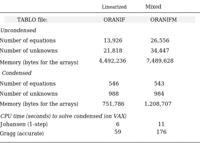
All figures reported here refer to the 23 commodity, 22 sector and 2 occupation version. The figures discussed here are shown in Table 5.1.
As can be seen, the mixed representation has approximately twice as many equations as the linear one and approximately 50 per cent more unknowns. To solve the mixed version directly would require approximately 7.5 megabytes (Mb) of memory compared to approximately 4.5Mb for the linear one.
However, models of the size of ORANI-F are almost never solved directly in their original form. Rather they are first reduced in size using the
G
EMPACKcondensation facility. In the latter, endogenous variables whose values are not of great interest [typically having 2 or more arguments such as P1CSI(i,s,j)] are substituted out symbolically before any arithmetic calculations are carried out. (See section 6 of HPP or chapter 3 of Harrison and Pearson (1993a) for more details.)
8 In the linearized TABLO Input file in HPP, w4tax_c is defined as the percentage change in the tax revenue. By contrast, in the mixed TABLO Input file ORANIFM.TAB, W4TAX_C is defined as the total dollar value of this revenue.
We chose a condensation of ORANIFM which leaves essentially the same equations and variables as in the condensation of the linear version used in HPP. The numbers of unknowns and equations are shown in Table 5.1. Again the mixed version requires more memory (about 1.2Mb) for its arrays than the linear one (about 0.75Mb).
We carried out several of the simulations in HPP using both representations. The numerical results were the same (taking into account machine and solution-method accuracy) which confirmed that the two versions actually represent the same model. Table 5.1 reports the CPU (processing) times on our VAX computer for
Table 5.1
Comparing Linear and Mixed Implementations of ORANI-F
Linearized Mixed
TABLO file: ORANIF ORANIFM
Uncondensed
Number of equations 13,926 26,556
Number of unknowns 21,818 34,447
Memory (bytes for the arrays) 4,492,236 7,489,628
Condensed
Number of equations 546 543
Number of unknowns 988 984
Memory (bytes for the arrays) 751,786 1,208,707
CPU time (seconds) to solve condensed (on VAX)
Johansen (1-step) 6 11
Gragg (accurate) 59 176
doing a typical Johansen (1-step) and an accurate nonlinear solution (Gragg 8,10, 12-step followed by extrapolation) with the two versions. The linear one solves more quickly in each case.
By comparison with the older version of TABLO which required users to present nonlinear equations in linearized form, relatively little experience has so far accumulated with the use of the new levelsfacility with large models. The ORANI-F experience, that our initial mixed representation requires more CPU and memory to solve than an efficient linear one, may turn out to be generally true. It is also possible that mixed implementations will become more efficient when the levels/mixed version of the software matures and modellers gain more experience with it.
6. Conclusion
It is now practical to implement models in
G
EMPACK using a linear representation, a levels representation or a mixed levels/linear representation.TABLO Input files are perhaps easiest to construct in mixed mode where accounting identities are expressed directly (in levels form) and behavioural equations are expressed most succinctly (which usually means in linearized form). In view of their relative transparency, files using the mixed approach are likely to be more satisfactory as documentation and a better vehicle for transferring models to other users.
The great advantage of using a levels or mixed representation is that modellers don’t have to work out the linearizations by hand;
G
EMPACK now does it automatically and more reliably. We have found that relatively inexperienced modellers can implement a model much more quickly and easily using a levels or mixed representation. The implementation of AIDADS in section 4 above shows clearly that a pure levels implementation has distinct advantages for some models.References
Brooke, Anthony, David Kendrick and Alexander Meeraus (1988) GAMS: A User’s Guide, The Scientific Press, Redwood City.
Codsi, G. and K. R. Pearson (1988) "GEMPACK: General-Purpose Software for Applied General Equilibrium and Other Economic Modellers",
Computer Science in Economics and Management, Vol. 1, pp. 189-207.
Cooper, R.J. and K.R. McLaren (1992a) “An Empirically Oriented Demand System with Improved Regularity Properties”, Canadian Journal of Economics, Vol. 25, pp. 652-67.
Cooper, R. J. and K. R. McLaren (1992b) "A System of Demand Equations Satisfying Effectively Global Regularity Conditions", Department of Econometrics, Monash University, mimeo (July).
Dixon, P.B., B.R. Parmenter, A.A. Powell and P.J. Wilcoxen (1992) Notes and Problems in Applied General Equilibrium Economics, North-Holland, Amsterdam.
Dixon, P.B., B.R. Parmenter, J. Sutton and D.P. Vincent (1982) ORANI: A Multisectoral Model of the Australian Economy, North-Holland, Amsterdam.
Harrison, W. Jill and K.R. Pearson (1993a) “An Introduction to GEMPACK”, GEMPACK document GPD-1, First edition, Impact Project, April 1993, pp. 182+14.
Harrison, W. Jill and K.R. Pearson (1993b) “User’s Guide to TABLO and TABLO-generated Programs”, GEMPACK document GPD-2, First edition, Impact Project, April 1993, pp. 110+12.
Harrison, W. Jill and K.R. Pearson (1993c) “Implementing Levels Models Directly using GEMPACK”, GEMPACK document GPD-4, First edition, Impact Project, April 1993, pp. 55+7.
Hertel, T.W., J.M. Horridge and K.R. Pearson (1992) “Mending the Family Tree: A Reconciliation of the Linearized and Levels School of AGE Modelling”, Economic Modelling, Vol. 9, pp. 385-407.
Horridge, J. M., B. R. Parmenter and K. R. Pearson (1993) "ORANI-F: A General Equilibrium Model of the Australian Economy", Economic and Financial Computing, Vol. 3, pp.71-140.
Parmenter, B. R. (1988) "ORANI-F User's Manual", Institute of Applied Economic and Social Research, University of Melbourne, Working Paper No.7/88, (August), 59 pp.
Rimmer, M. T. and A. A. Powell (1992a) "An Implicitly Directly Additive Demand System: Estimates for Australia", Impact Project Preliminary Working Paper No. OP-73, Monash University (October). Rimmer, M. T. and A. A. Powell (1992b) "Demand Patterns across the Development Spectrum: Estimates of the AIDADS System", Impact Project Preliminary Working Paper No. OP-75, Monash University (October).