On the Power of Multiple Anonymous Messages

(1)

On the Power of Multiple Anonymous Messages

∗

Badih Ghazi Noah Golowich† Ravi Kumar Rasmus Pagh‡ Ameya Velingker Google Research

Mountain View, CA

[email protected], [email protected], [email protected], [email protected], [email protected]

Abstract

An exciting new development in differential privacy is theshuffledmodel, in which an anonymous channel enables non-interactive, differentially private protocols with error much smaller than what is possible in the local model, while relying on weaker trust assumptions than in the central model. In this paper, we study basic counting problems in the shuffled model and establish separations between the error that can be achieved in the single-message shuffled model and in the shuffled model with multiple single-messages per user.

For the problem offrequency estimationfornusers and a domain of sizeB, we obtain:

• A nearly tight lower bound ofΩ˜pminp?4_n,?_B_qq_{on the error in the single-message shuffled model. This}

implies that the protocols obtained from the amplification via shuffling work of Erlingsson et al. (SODA 2019) and Balle et al. (Crypto 2019) are essentially optimal for single-message protocols. A key ingredient in the proof is a lower bound on the error of locally-private frequency estimation in the low-privacy (aka highε) regime. For this we develop new techniques to extend the results of Duchi et al. (FOCS 2013; JASA 2018) and Bassily & Smith (STOC 2015), whose techniques were restricted to the high-privacy case. • Protocols in themulti-messageshuffled model withpolyplogB,lognqbits of communication per user and

poly logB error, which provide an exponential improvement on the error compared to what is possible with single-message algorithms. This implies protocols with similar error and communication guarantees for several well-studied problems such as heavy hitters,d-dimensional range counting, M-estimation of the median and quantiles, and more generally sparse non-adaptive statistical query algorithms.

For the relatedselectionproblem on a domain of sizeB, we prove:

• A nearly tight lower bound ofΩpBqon the number of users in the single-message shuffled model. This significantly improves on theΩpB1{17

qlower bound obtained by Cheu et al. (Eurocrypt 2019), and when combined with theirO˜p

?

Bq-error multi-message protocol, implies the first separation between single-message and multi-single-message protocols for this problem.

∗

A1-page abstract based on this work will be presented at the Symposium on Foundations of Responsible Computing (FORC) 2020.

†

MIT EECS. Supported at MIT by a Fannie & John Hertz Foundation Fellowship, an MIT Akamai Fellowship, and an NSF Graduate Fellowship. This work was done while at Google Research.

‡

Visiting from BARC and IT University of Copenhagen.

(2)

1 Introduction

With increased public awareness and the introduction of stricter regulation of how personally identifiable data may be stored and used, user privacy has become an issue of paramount importance in a wide range of practical applications.

While many formal notions of privacy have been proposed (see, e.g., [LLV07]),differential privacy (DP)[DMNS06,

DKM`_{06] has emerged as the gold standard due to its broad applicability and nice features such as composition and}

post-processing (see, e.g., [DR`_{14b, Vad17] for a comprehensive overview). A primary goal of DP is to enable}

processing of users’ data in a way that (i) does not reveal substantial information about the data of any single user, and (ii) allows the accurate computation of functions of the users’ inputs. The theory of DP studies what trade-offs between privacy and accuracy are feasible for desired families of functions.

Most work on DP has been in thecentral(a.k.a. curator) setup, where numerous private algorithms with small

error have been devised (see, e.g., [BLR08, DNR`_{09, DR14a]). The premise of the central model is that a curator}

can access the raw user data before releasing a differentially private output. In distributed applications, this requires users to transfer their raw data to the curator — a strong limitation in cases where users would expect the entity running the curator (e.g., a government agency or a technology company) to gain little information about their data.

To overcome this limitation, recent work has studied the localmodel of DP [KLN`_{08] (also [War65]), where}

each individual message sent by a user is required to be private. Indeed, several large-scale deployments of DP in practice, at companies such as Apple [Gre16, App17], Google [EPK14, Sha14], and Microsoft [DKY17], have used local DP. While estimates in the local model require weaker trust assumptions than in the central model, they inevitably suffer from significant error. For many types of queries, the estimation error is provably larger than the error incurred in the central model by a factor growing with the square root of the number of users.

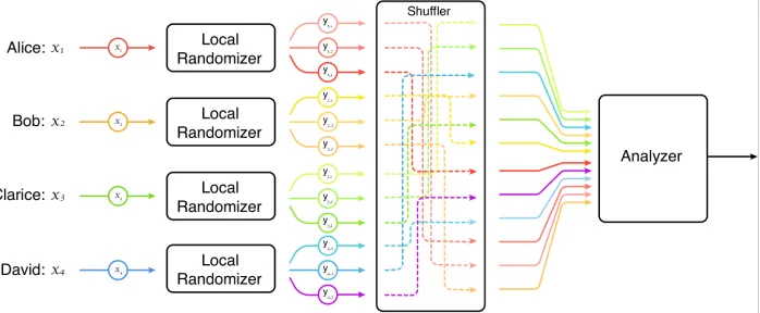
Shuffled Privacy Model. The aforementioned trade-offs have motivated the study of theshuffledmodel of privacy as a middle ground between the central and local models. While a similar setup was first studied in cryptography in the work of Ishai et al. [IKOS06] on cryptography from anonymity, the shuffled model was first proposed for privacy-preserving protocols by Bittau et al. [BEM`_{17] in their Encode-Shuffle-Analyze architecture. In the shuffled setting,}

each user sends one or more messages to the analyzer using ananonymouschannel that does not reveal where each

message comes from. This kind of anonymization is a common procedure in data collection and is easy to explain to regulatory agencies and users. The anonymous channel is equivalent to all user messages being randomly shuffled (i.e., permuted) before being operated on by the analyzer, leading to the model illustrated in Figure 1; see Section 2.2 for a formal description of the shuffled model. In this work, we treat the shuffler as a black box, but note that various efficient cryptographic implementations of the shuffler have been considered, including onion routing, mixnets,

third-party servers, and secure hardware (see, e.g., [IKOS06, BEM`_{17]). A comprehensive overview of recent work}

on anonymous communication can be found on Free Haven’s Selected Papers in Anonymity website1.

1_{https://www.freehaven.net/anonbib/}

(4)

The DP properties of the shuffled model were first analytically studied, independently, in the works of Erlingsson

et al. [EFM`_{19] and Cheu et al. [CSU}`_{19]. Protocols within the shuffled model are non-interactive and fall into}

two categories: single-messageprotocols, in which each user sends one message (as in the local model), and

multi-messageprotocols, in which a user can send more than one message. In both variants, the messages sent by all users are shuffled before being passed to the analyzer. The goal is to design private protocols in the shuffled model with as small error and total communication as possible. An example of the power of the shuffled model was established

by Erlingsson et al. [EFM`_{19] and extended by Balle et al. [BBGN19c], who showed that every local DP algorithm}

directly yields a single-message protocol in the shuffled model with significantly better privacy.

1.1 Results

In this work, we study several basic problems related tocountingin the shuffled model of DP. In these problems,

each of n users holds an element from a domain of size B. We consider the problems of frequency estimation,

variable selection, heavy hitters, median, and range counting and study whether it is possible to obtainpε, δq-DP2_in

the shuffled model with accuracy close to what is possible in the central model, while keeping communication low. The frequency estimation problem (a.k.a. histograms orfrequency oracles) is at the core of all the problems we study. In the simplest version, each ofnusers gets an element of a domainrBs :“ t1, . . . , Buand the goal is

to estimate the number of users holding elementj, for any query elementj P rBs. Frequency estimation has been

extensively studied in DP where in the central model, the smallest possible error isΘpminplogp1{δq{ε,logpBq{ε, nqq

(see, e.g., [Vad17, Section 7.1]). By contrast, in the local model of DP, the smallest possible error is known to be

ΘpminpanlogpBq{ε, nqunder the assumption thatδă1{n[BS15].

In the high-level exposition of our results given below, we letnandB be any positive integers,ε ą 0be any

constant, andδ ą 0 be inverse polynomial inn. This assumption on εandδ covers a regime of parameters that

is relevant in practice. We will also make use of tilde notation (e.g.,O˜,Θ˜) to indicate the possible suppression of multiplicative factors that are polynomial inlogBandlogn.

Single-Message Bounds for Frequency Estimation. For the frequency estimation problem, we show the follow-ing results in the shuffled model where each user sends a sfollow-ingle message.

Theorem 1.1(Informal version of Theorems 3.1 & 3.4). The optimal error of private frequency estimation in the single-message shuffled model isΘpminp˜ ?4_n,?_B

qq.

The main contribution of Theorem 1.1 is the lower bound. To prove this result, we obtain improved bounds

on the error needed for frequency estimation in local DP in the weak privacy regime whereεis aroundlnn. The

upper bound in Theorem 1.1 follows by combining the recent result of Balle et al. [BBGN19c] (building on the

earlier result of Erlingsson et al. [EFM`_{19]) with RAPPOR [EPK14] and}_B_{-ary randomized response [War65] (see}

Section 1.2 and Appendix A for more details).

Theorem 1.1 implies that in order for a single-message differentially private protocol to get erroropnqone needs

to haven“ω

´

logB log logB

¯

users; see Corollary 3.2. This improves on a result of Cheu et al. [CSU`_{19, Corollary 32],}

which gives a lower bound ofn“ωplog1{17Bqfor this task.

Single-Message Bounds for Selection. It turns out that the techniques that we develop to prove the lower bound

in Theorem 1.1 can be used to get a nearly tightΩpBqlower bound on the number of users necessary to solve the

selectionproblem. In the selection problem3, each useri P rnsis given an arbitrary subset ofrBs, represented by the indicator vectorxi P t0,1uB, and the goal is for the analyzer to output an indexj˚P rBssuch that

ÿ

iPrns

xi,j˚ ěmax jPrBs

ÿ

iPrns

xi,j´

n

10. (1)

2

Formally stated in Definition 2.1.

3

(5)

In other words, the analyzer’s output should be the index of a domain element that is held by an approximately

maximal number of users. The choice of the constant10in (1) is arbitrary; any constant larger than1may be used.

The selection problem has been studied in several previous works on differential privacy, and it has many ap-plications to machine learning, hypothesis testing and approximation algorithms (see [DJW13, SU17, Ull18] and

the references therein). Our work improves anΩpB1{17qlower bound in the single-message shuffled model due to

Cheu et al. [CSU`_{19]. For}_ε

“1, the exponential mechanism [MT07] implies anpε,0q-DP algorithm for selection

withn“OplogBqusers in the central model, whereas in the local model, it is known that anypε,0q-DP algorithm

for selection requiresn “ ΩpBlogBqusers [Ull18]. Variants of the selection problem appear in several natural

statistical tasks such as feature selection and hypothesis testing (see, e.g., [SU17] and the references therein).

Theorem 1.2 (Informal version of Theorem 3.22). For any single-message differentially private protocol in the shuffled model that solves the selection problem given in Equation (1), the numbernof users should beΩpBq.

The lower bound in Theorem 1.2 nearly matches theOpBlogBqupper bound on the required number of users

that holds even in the local model (and hence in the single-message shuffled model) and that uses theB-randomized

response [War65, Ull18]. Cheu et al. [CSU`_{19] have previously obtained a multi-message protocol for selection}

withOp?Bqusers, and combined with this result Theorem 1.2 yields the first separation between single-message

and multi-message protocols for selection.

Multi-Message Protocols for Frequency Estimation. We next present (non-interactive) multi-message protocols

in the shuffled model of DP for frequency estimation with onlypolylogarithmicerror and communication. This is

in strong contrast with what is possible for any protocol in the single-message shuffled setup where Theorem 1.1

implies that the error has to grow polynomially withminpn, Bq, even with unbounded communication. In addition

to error and communication, a parameter of interest is the query time, which is the time to estimate the frequency of any elementj P rBsfrom the data structure constructed by the analyzer.

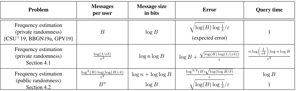
Theorem 1.3(Informal version of Theorems 4.1 & 4.2). There is a private-coin (resp., public-coin) multi-message protocol in the shuffled model for frequency estimation with errorO˜p1q, total communication ofO˜p1qbits per user, and query timeO˜pnq(resp.,O˜p1q).

Combining Theorems 1.1 and 1.3 yields the first separation between single-message and multi-message protocols for frequency estimation. Moreover, Theorem 1.3 can be used to obtain multi-message protocols with small error and small communication for several other widely studied problems (e.g., heavy hitters, range counting, and median and quantiles estimation), discussed in Section 1.4. Finally, Theorem 1.3 implies the following consequence for

statistical query (SQ) algorithms with respect to a distributionDon X (see Appendix B for the basic definitions).

We say that a non-adaptive SQ algorithmAmaking at mostBqueriesq :X Ñ t0,1uisk-sparseif for eachxPX,

the Hamming weight of the output of the queries is at mostk. Then, under the assumption that users’ data is drawn

i.i.d. fromD, the algorithmAcan be efficiently simulated in the shuffled model as follows:

Corollary 1.4(Informal version of Corollary B.1). For any non-adaptivek-sparse SQ algorithmAwithB queries andβ ą0, there is a (private-coin) shuffled model protocol satisfyingpε, δq-DP whose output has total variation dis-tance at mostβ from that ofA, such that the number of users isnďO˜`_ετk `_τ12

˘

, and the per-user communication

isO˜

´

k2 ε2

¯

, whereO˜p¨qhides logarithmic factors inB, n,1{δ,1{ε, and1{β.

Corollary 1.4 improves upon the simulation of non-adaptive SQ algorithms in thelocal model[KLN`_{08], for}

which the number of users must grow as _ε2k_τ2 as opposed to _τ12 ` _ετk in the shuffled model. We emphasize that

the main novelty of Corollary 1.4 is in the regime that k2{ε2 ! B; in particular, though prior work on

low-communication private summation in the shuffled model [CSU`_{19, GMPV19, BBGN20] implies an algorithm for}

simulatingAwith roughly the same bound on the number of usersnas in Corollary 1.4 and communicationΩpBq,

it was unknown whether the communication could be reduced to have logarithmic dependence onB, as in Corollary

(6)

Local Local + shuffle Shuffled, single-message

Shuffled,

multi-message Central

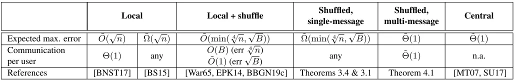
Expected max. error O˜p?nq Ω˜p?nq O˜pminp?4_n,?_B_qq _Ω˜_p_min_p?4_n,?_B_qq _Θ˜_p₁_q _Θ˜_p₁_q

Communication

per user Θp1q any

OpBq(err?4_n₎

˜

Op1q(err?B) any Θ˜p1q n.a.

References [BNST17] [BS15] [War65, EPK14, BBGN19c] Theorems 3.4 & 3.1 Theorem 4.1 [MT07, SU17]

Table 1: Upper and lower bounds on expected maximum error (over all B queries, where the sum of all frequencies isn) for frequency estimation in different models of DP. The bounds are stated for fixed, positive privacy parametersεandδ, and

˜

Θ{O˜{Ω˜ asymptotic notation suppresses factors that are polylogarithmic inBandn. The communication per user is in terms of the total number of bits sent. In all upper bounds, the protocol is symmetric with respect to the users, and no public randomness is needed. References are to the first results we are aware of that imply the stated bounds.

1.2 Overview of Single-Message Lower Bounds

We start by giving an overview of the lower bound ofΩpmint˜ n1{4,?Buqin Theorem 1.1 on the error of any

single-message frequency estimation protocol. We first focus on the case wherenďB2 and thusmintn1{4,?Bu “n1{4.

The main component of the proof in this case is a lower bound ofΩp˜ n1{4qfor frequency estimation forpεL, δLq-local

DP protocols4when εL “ lnpnq `Op1q. While lower bounds for local DP frequency estimation were previously

obtained in the seminal works of Bassily and Smith [BS15] and Duchi, Jordan and Wainwright [DJW18], two critical

reasons make them less useful for our purposes: (i) their dependence onεLis sub-optimal whenεL “ ωp1q(i.e.,

low error regime) and (ii) they only apply to the case whereδL“0(i.e., pure privacy).5 We prove new error bounds

in the low error and approximate privacy regime in order to obtain our essentially tight lower bound in Theorem 1.1 for single-message shuffled protocols. We discuss these and outline the proof next.

LetRbe anpεL, δLq-locally differentially private randomizer. The general approach [BS15, DJW18] is to show

that ifV is a random variable drawn uniformly at random fromrBsand ifX is a random variable that is equal to

V with probability parameterα P p0,1q, and is drawn uniformly at random fromrBsotherwise, then the mutual

information betweenV and the local randomizer outputRpXqsatisfies

IpV;RpXqq ď logB

4n . (2)

Once (2) is established, the chain rule of mutual information implies thatIpV;RpX1q, . . . , RpXnqq ď log₄B, where

X1, . . . , Xn are independent and identically distributed given V. Fano’s inequality [CT91] then implies that the

probability that any analyzer receivingRpX1q, . . . , RpXnqcorrectly guesses V is at most1{4; on the other hand,

an Ωpαnq-accurate analyzer must be able to determineV with high probability since its frequency in the dataset

X1, . . . , Xnis roughlyαn, greater than the frequency of all othervP rBs. This approach thus yields a lower bound

ofΩpαnqon frequency estimation.

To prove the desiredΩp˜ n1{4_q_{lower bound using this approach, it turns out we need a bound of the form}

IpV;RpXqq ďO˜pα4neεL_q_, ₍₃₎

where bothδL ą 0 andεL “ ωp1q. (We will in fact chooseα “ Θp˜ n´3{4q andεL “ lnpnq `Op1q; as we will

discuss later, (3) is essentially tight in this regime.)

Limitations of Previous Approaches We first state the existing upper bounds onIpV;RpXqq, which only use the

privacy of the local randomizer. Bassily and Smith [BS15, Claim 5.4] showed an upper bound ofIpV;RpXqq ď

Opε2_Lα2qwithεL “ Op1qandδL “op1{pnlognqq, which thus satisfies (2) withα “ Θ

´b

logB ε2

Ln

¯

. ForδL “ 0,

4

Note that we use the subscripts inεLandδLto distinguish the privacy parameters of thelocalmodel from theεandδparameters (without

a subscript) of the shuffled model.

5

As we discuss in Remark 3.1, generic reductions [CSU`_{19, BNS18] showing that one can efficiently simulate an approximately}

differ-entially private protocol (i.e., withδLą0) with a pure differentially private protocol (i.e., withδL“0) are insufficient to obtain tight lower

(7)

Duchi et al. [DJW18] generalized this result to the caseεLě1, proving that6IpV;RpXqq ďOpα2e2εLq. Both of

these bounds are weaker than (3) for the above setting ofαandεL.

However, proving the mutual information bound in (3) turns out to be impossible if we only use the privacy of the local randomizers! In fact, the bound can be shown to befalseif all we assume aboutRis that it ispεL, δLq-locally

differentially private for someεL « lnnandδL “ n´Op1q. For instance, it is violated if one takesR to beRRR,

the local randomizer of theB-randomized response [War65]. Consider for example the regime whereB ďnďB2,

and the setting where RRRpvq is equal to v with probability 1´B{n, and is uniformly random over rBs with

the remaining probability of B{n. In this case, the local randomizer RRRp¨q is plnpnq `Op1q,0q-differentially

private. A simple calculation shows thatIpV;RRRpXqq “ Θp˜ αq. Wheneverα !1{ ?

n, which is the regime we

have to consider in order to obtain any non-trivial lower bound7in the single-message shuffled model, it holds that

α " α4nexpplnpnqq, thus contradicting (3) (see Remark 3.4). The insight derived from this counterexample is actually crucial, as we describe in our new technique next.

Mutual Information Bound from Privacy and Accuracy Departing from previous work, we manage to prove the

stronger bound (3) as follows. Inspecting the counterexample based on theB-randomized response outlined above,

we first observe that any analyzer in this case must have error at leastΩp?Bq, which is larger thanαn, the error that would be ruled out by the subsequent application of Fano’s inequality! This led us to appeal to accuracy, in addition to privacy, when proving the mutual information upper bound. We thus leverage the additional available property that the local randomizerR can be combined with an analyzerAin such a way that the mappingpx1, . . . , xnq ÞÑ

ApRpx1q, . . . , Rpxnqqcomputes the frequencies of elements of every datasetpx1, . . . , xnqaccurately, i.e., to within

an error ofOpαnq. At a high level, our approach for proving the bound in (3) then proceeds by:

(i) Proving a structural property satisfied by the randomizer corresponding to any accurate frequency estimation protocol. Namely, we show in Lemma 3.15 that if there is an accurate analyzer, the total variation distance between the output of the local randomizer on any given input, and its output on a uniform input, is close to 1. (ii) Using thepεL, δLq-DP property of the randomizer along with the structural property in (i) in order to

upper-bound the mutual informationIpV;RpXqq.

We believe that the application of the structural property in (i) to proving bounds of the form (3) is of independent interest. As we further discuss below, this property is, in particular, used (together with privacy ofR) to argue that for most inputsv P rBs, the local randomizer outputRpvq is unlikely to equal a message that is much less likely

occur when the input is uniformly random than when it isv. Note that it is somewhat counter-intuitive that accuracy

is used in the proof of this fact, as one way to achieve very accurate protocols is to ensure thatRpvq is equal to a

message which is unlikely when the input is anyu‰v. We now outline the proofs of (i) and (ii) in more detail.

The gist of the proof of (i) is an anti-concentration statement. Let vbe a fixed element ofrBsand letX be a

random variable uniformly distributed onrBs. Assume that the total variation distance∆pRpvq, RpXqqis not close

to1, and that a small fraction of the users have inputvwhile the rest have uniformly random inputs. LetZdenote

the range of the local randomizerR. First, we consider the special case whereZ ist0,1u. Then the distribution of the shuffled outputs of the users withvas their input is in bijection with a binomial random variable with parameter

p:“PrRpvq “1s, and the same is true for the distribution of the shuffled outputs of the users with uniform random

inputsX (with parameterq :“PrRpXq “1s). Then, we use the anti-concentration properties of binomial random

variables in order to argue that if|p´q| “∆pRpvq, RpXqqis too small, then with nontrivial probability the shuffled outputs of the users with inputvwill be indistinguishable from the shuffled outputs of the users with uniform random inputs. This is then used to contradict the supposed accuracy of the analyzer. To deal with the general case where the rangeZ is any finite set, we repeatedly apply the data processing inequality for total variation distance in order to reduce to the binary case (Lemma 3.20). The full proof appears in Lemma 3.15.

Equipped with the property in (i), we now outline the proof of the mutual information bound in (ii). Denote by

• T_vthe set of messagesmuch more likelyto occur when the input isvthan when it is uniform,

• Yvthe set of messagesless likelyto occur when the input isvthan when it is uniform.

6

This bound is not stated explicitly in [DJW18], though [DJW18, Lemma 7] proves a similar result whose proof can readily be modified appropriately.

(8)

Note that the unionT_vYYvisnotthe entire rangeZof messages; in particular, it does not include messages that are

a bit more likelyto occur when the input isvthan when it is uniform.8 On a high level, it turns out that the mutual informationIpV;RpXqqwill be large, i.e.,RpXqwill reveal a significant amount of information aboutV, if either of the following events occurs:

(a) There are too many inputsvP rBssuch that the massPrRpXq PYvsis small. Intuitively, for suchv, the local

randomizerRfails to “hide” the fact that a uniform inputXisvgiven thatXindeed equalsvandRpXq PYv.

(b) There are too many inputsv P rBssuch that the massPrRpvq PTvsis large. Such inputs make it too likely

thatX“vgiven thatRpXq PTv, which makes it more likely in turn thatV “v.

We first note that the total variation distance∆pRpvq, RpXqqis upper-bounded byPrRpXq P Yvs. On the other

hand, the accuracy of the protocol along with property (i) imply that∆pRpvq, RpXqqis close to1. By putting these together, we can conclude that event (a) does not occur (see Lemma 3.15 for more details).

To prove that event (b) does not occur, we use the pεL, δLq-DP guarantee of the local randomizerR. Namely,

we will use the inequalityPrRpvq P Ss ď eεL _¨

PrRpXq P Ss `δ for various subsets S ofZ. Unfortunately,

settingS “ Tv does not lead to a good enough upper bound onPrRpvq P Tvs; indeed, for the local randomizer

R “ RRRcorresponding to theB-ary randomized response, we will haveTv “ tvuforn "B, and soPrRpvq P

Tvs “ 1´B{n « 1for anyv. Thus, to establish (b), we need to additionally use the accuracy of the analyzerA

(i.e., property (i) above), together with a careful double-counting argument to enumerate the probabilities thatRpvq

belongs to subsets ofTv of different granularity (with respect to the likelihood of occurrence under inputvversus a

uniform input). For the details, we refer the reader to Section 3.3 and Lemma 3.14.

Having established the above lower bound for locally differentially private estimation in the low-privacy regime,

the final step is to apply a lemma of Cheu et al. [CSU`_{19] (restated as Lemma 3.5 below), stating that any lower}

bound forpε`lnpnq, δq-locally differentially private protocols implies a lower bound forpε, δq-differentially private protocols in the single-message shuffled model (i.e., we takeεL “ε`lnpnq). Moreover, forεL “lnpnq `Op1q

andα “ Θp˜ n´3{4q, we observe that (3) implies (2), and thus a lower bound of Ωp˜ αnq “ Ωp˜ n1{4qfor frequency estimation in the single-message shuffled model follows. Finally, we point out that while the above outline focused

on the case wheren ď B2, it turns out that this is essentially without loss of generality as the other case where

nąB2can be reduced to the former (see Lemma 3.10).

Tightness of Lower Bounds The lower bounds sketched above are nearly tight. The upper bound of Theorem 1.1 follows from combining existing results showing that the single-message shuffled model provides privacy

ampli-fication of locally differentially private protocols [EFM`_{19, BBGN19c], with known locally differentially private}

protocols for frequency estimation [War65, EPK14, DJW18, BBGN19c]. In particular, as recently shown by Balle et al. [BBGN19c], a purepεL,0q-differentially private local randomizer yields a protocol in the shuffled model that

is ˆ

O

ˆ

eεL

b

logp1{δq n

˙

, δ

˙

-differentially private and that has the same level of accuracy.9 Then:

• When combined with RAPPOR [EPK14, DJW18], we get an upper bound ofO˜pn1{4_q_{on the error.}

• When combined with theB-randomized response [War65, ASZ19], we get an error upper bound ofO˜p?Bq.

The full details appear in Appendix A. Put together, these imply that the minimum in our lower bound in Theorem 1.1 is tight (up to logarithmic factors). It also follows that the mutual information bound in Equation (3) is tight (up to

logarithmic factors) forεL “ lnpnq `Op1q andα “ n´3{4 (which is the parameter settings corresponding to the

single-message shuffled model); indeed, a stronger bound in Equation (3) would lead to larger lower bounds in the single-message shuffled model thereby contradicting the upper bounds discussed in this paragraph.

Lower Bound for Selection: Sharp Bound on Level-1 Weight of Probability Ratio Functions We now outline

the proof of the nearly tight lower bound on the number of users required to solve the selection problem in the

8

For clarity of exposition in this overview, we refrain from quantifying the likelihoods in each of these cases; for more details on this, we refer the reader to Section 3.3.

9

Note that we cannot use the earlier amplification by shuffling result of [EFM`19], since it is only stated forεL“Op1qwhereas we need

(9)

single-message shuffled model (Theorem 1.2). The main component of the proof in this case is a lower bound of

ΩpBqusers for selection forpεL, δLq-localDP protocols whenεL“lnpnq `Op1q.

In the case of localpεL,0q-DP (i.e., pure) protocols, Ullman [Ull18] proved a lower boundn“Ω

´

BlogB pexppεLq´1q2

¯ . There are two different reasons why this lower bound is not sufficient for our purposes:

1. It does not rule out DP protocols withδL ą0(i.e., approximate protocols), which are necessary to consider

for our application to the shuffled model.

2. For the low privacy setting ofεL “lnpnq `Op1q, the bound simplifies ton“Ωp˜ B{n2q, i.e.,n“Ωp˜ B1{3q,

weaker than what we desire.

To prove our near-optimal lower bound, we remedy both of the aforementioned limitations by allowing positive

values ofδLand achieving a better dependence onεL. As in the proof of frequency estimation, we reduce proving

Theorem 1.2 to the task of showing the following mutual information upper bound:

IppL, Jq;RpXL,Jqq ďO˜

ˆ

1

B

˙

`OpδLpB`nqq, (4)

whereLis a uniform random bit,J is a uniform random coordinate inrBs, andXL,J is uniform over the subcube

tx P t0,1uB : xJ “ Lu. Indeed, once (4) holds and δL ă op1{pBnqq, the chain rule implies that the mutual

information between all users’ messages and the pairpL, Jqis at mostO

´

nlnpBq B

¯

. It follows by Fano’s inequality that ifn“opBq, no analyzer can determine the pairpL, Jqwith high probability (which any protocol for selection must be able to do).

For any messagezin the range ofR, define the Boolean functionfzpxq:“ _P_rRpXPrRpxq“zs

L,Jq“zs wherexP t0,1u B_{. Let} W1rfsdenote the level-1Fourier weight of a Boolean function f. To prove inequalities of the form (4), the prior work of Ullman [Ull18] shows thatIppL, Jq;RpXL,Jqqis determined byW1rfzs, up to normalization constants. In

the case whereδL“0andεL“lnpnq `Op1q,fz P r0, eεLs, and by Parseval’s identityW1rfzs ďOpe2εLqfor any

messagez, leading to

IppL, Jq;RpXL,Jqq ďO

ˆ

e2εL

B

˙

. (5)

Unfortunately, for our choice ofεL“lnpnq `Op1q, (5) is weaker than (4).

To show (4), we depart from the previous approach in the following ways:

(a) We show that the functionsfz take values inr0, OpeεLqsformostinputsx; this uses thepεL, δLq-local DP of

the local randomizerR.

(b) Using theLevel-1inequalityfrom the analysis of Boolean functions [O’D14] (see Theorem 3.26 below), we

upper boundW1rgzsbyOpεLq, wheregzis the truncation offz defined bygzpxq “fzpxqiffzpxq ďOpnq,

andgzpxq “0otherwise.

(c) We boundIppL, Jq;RpXL,JqqbyW1rgzs, using the factfz is sufficiently close to its truncationgz.

The above line of reasoning, formalized in Section 3.5, allows us to show

IppL, Jq;RpXL,Jqq ďO

´ε

L

B `δ¨ pB`e

εL_q

¯

,

which is sufficient to establish that (4) holds.

Having proved a lower bound on the error of anypε`lnn, δq-local DP protocol for selection withε “Op1q,

the final step in the proof is to apply a lemma of [CSU`_{19] to deduce the desired lower bound in the single-message}

shuffled model.

1.3 Overview of Multi-Message Protocols

An important consequence of our lower bound in Theorem 1.1 is that one cannot achieve an error ofO˜p1q using

single-messageprotocols. This in particular rules out any approach that uses the following natural two-step recipe for getting a private protocol in the shuffled model with accuracy better than in the local model:

(10)

2. Randomly shuffle the messages obtained when each user runs step 1 on their input, and use the privacy

amplification by shuffling bounds [EFM`_{19, BBGN19c] to improve the privacy guarantees.}

Thus, shuffled versions of theB-randomized response [War65, ASZ19], RAPPOR [EPK14, DJW18, ASZ19], the

Bassily–Smith protocol [BS15], TreeHist and Bitstogram [BNST17], and the Hadamard response protocol [ASZ19, AS19], will still incur an error ofΩpminp?4_n,?_B

qq.

Moreover, although the single-message protocol of Cheu et al. [CSU`_{19] for binary aggregation (as well as}

the multi-message protocols given in [GPV19, BBGN19a, GMPV19, BBGN19b] for the more general task of real-valued aggregation) can be applied to the one-hot encodings of each user’s input to obtain a multi-message protocol

for frequency estimation with errorO˜p1q, the communication per user would beΩpBqbits, which is clearly

unde-sirable.

Recall that the main idea behind (shuffled) randomized response is for each user to send their input with some probability, and random noise with the remaining probability. Similarly, the main idea behind (shuffled) Hadamard response is for each user to send a uniformly random index from the support of the Hadamard codeword correspond-ing to their input with some probability, and a random index from the entire universe with the remaincorrespond-ing probability. In both protocols, the user is sending a message that either depends on their input or is noise; this restriction turns out to be a significant limitation. Our main insight is that multiple messages allows users to simultaneously send both types of messages, leading to a sweet spot with exponentially smaller error or communication.

Our protocols. We design a multi-message version of the private-coin Hadamard response of Acharya et al. [ASZ19,

AS19] where each user sends a small subset of indices sampled uniformly at random from the support of the

Hadamard codeword corresponding to their input, and in addition sends a small subset of indices sampled uniformly at random from the entire universerBs. To get accurate results it is crucial that a subset of indices is sampled, as opposed to just a single index (as in the local model protocol of [ASZ19, AS19]). We show that in the regime where the number of indices sampled from inside the support of the Hadamard codeword and the number of noise indices sent by each user are both logarithmic, the resulting multi-message algorithm is private in the shuffled model, and it has polylogarithmic error and communication per user (see Theorem 4.1, Lemmas 4.4, 4.5, and 4.6 for more details). A limitation of our private-coin algorithm outlined above is that the time for the analyzer to answer a single query isO˜pnq. This might be a drawback in applications where the analyzer is CPU-limited or where it is supposed to produce real-time answers. In the presence of public randomness, we design an algorithm that remedies this limi-tation, having error, communication per user, and query time all equal toO˜p1q. Furthermore, the frequency estimates of this algorithm have one-sided error, and never underestimate the frequency of an element. This algorithm is based on a multi-message version of randomized response combined in a delicate manner with the Count Min data struc-ture [CM05a] (for more details, see Section 4.2). Previous work [BS15, BNST17] on DP have used Count Sketch [CCFC02], which is a close variant of Count Min, to go from frequency estimation to heavy hitters. In contrast, our use of Count Min has the purpose of reducing the amount of communication per user.

1.4 Applications

Heavy Hitters. Another algorithmic task that is closely related to frequency estimation is computing the heavy hitters in a dataset distributed across n users, where the goal of the analyzer is to (approximately) retrieve the identities and counts of all elements that appear at leastτ times, for a given thresholdτ. It is well-known that in

the central DP model, it is possible to computeτ-heavy hitters for anyτ “Θp1q˜ whereas in the local DP model, it

is possible to computeτ-heavy hitters if and only ifτ “Θp˜ ?nq. By combining with known reductions (e.g., from Bassily et al. [BNST17]), our multi-message protocols for frequency estimation yield multi-message protocols for

computing theτ-heavy hitters withτ “Θp1q˜ and total communication ofΘp1q˜ bits per user (for more details, see

Appendix D).

Range Counting. In range counting, each of thenusers is associated with a point in rBsd and the goal of the

(11)

in it?10 This is a basic algorithmic primitive that captures an important family of database queries and is useful in geographic applications. This problem has been well-studied in the central model of DP, where Chan et al. [CSS11] obtained an upper bound ofplogBqOpdqon the error (see Section 1.5 for more related work). It has also been studied in the local DP model [CKS19]; in this case, the error has to be at leastΩp?nqeven ford“1.

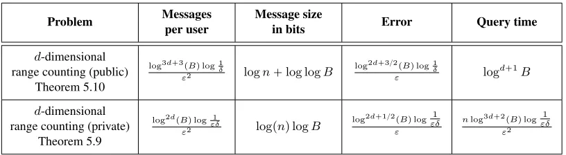
We obtain private protocols for range counting in the multi-message shuffled model with exponentially smaller error than what is possible in the local model (for a wide range of parameters). Specifically, we give a private-coin

multi-message protocol withplogBqOpdq messages per user each of length Oplognq bits, errorplogBqOpdq, and

query timeO˜pnlogdBq. Moreover, we obtain a public-coin protocol with similar communication and error but with a much smaller query time ofO˜plogdBq(see Section 5 for more details).

We now briefly outline the main ideas behind our multi-message protocols for range counting. We first argue

that even for d “ 2, the total number of queries is ΘpB2q and the number of possible queries to which a user

positively contributes is alsoΘpB2q. Thus, direct applications of DP algorithms for aggregation or for frequency

estimation would result in polynomial error and polynomial communication per user. Instead, we combine our multi-message protocol for frequency estimation (Theorem 1.3) with a communication-efficient implementation, in the multi-message shuffled model, of the space-partitioning data structure used in the central model protocol of Chan et al. [CSS11]. The idea is to use a collectionBofOpBlogdBqd-dimensional rectangles inrBsd(so-calleddyadic intervals) with the property that an arbitrary rectangle can be formed as the disjoint union ofOplogdBqrectangles fromB. Furthermore, each point inrBsdis contained inOplogdBqrectangles fromB. This means that it suffices to

release a private count of the number of points inside each rectangle inB— a frequency estimation task where each

user input contributes toOplogdBqbuckets. To turn this into a protocol with small maximum communication in

the shuffled model, we develop an approach analogous to the matrix mechanism [LHR`_{10, LM12]. We argue that}

the transformation of the aforementioned central model algorithm for range counting into a private protocol in the multi-message shuffled model with small communication and error is non-trivial and relies on the specific protocol structure. In fact, the state-of-the-art range counting algorithm of Dwork et al. [DNRR15] in the central model does not seem to transfer to the shuffled model.

M-Estimation of Median. A very basic statistic of any dataset of real numbers is its median. For simplicity,

suppose our dataset consists of real numbers lying in r0,1s. It is well-known that there is no DP algorithm for

estimating thevalueof the median of such a dataset with errorop1q(i.e., outputting a real number whose absolute

distance to the true median is op1q) [Vad17, Section 3]. This is because the median of a dataset can be highly

sensitive to a single data point when there are not many individual data points near the median. Thus in the context

of DP, one has to settle for weaker notions of median estimation. One such notion isM-estimation, which amounts to

finding a valuex˜that approximately minimizesř

i|xi´x˜|(recall that the median is the minimizer of this objective).

This notion has been studied in previous work on DP including by [Lei11, DJW18] (for more on related work, see Section 1.5 below). Our private range counting protocol described above yields a multi-message protocol with communicationO˜p1qper user and thatM-estimates the median up to error O˜p1q, i.e., outputs a valuey P r0,1s

such thatř_i|xi´y| ďmin˜x

ř

i|xi´x˜| `O˜p1q(see Theorem E.1 in Appendix E). BeyondM-estimation of the

median, our work implies private multi-message protocols for estimatingquantileswithO˜p1qerror andO˜p1qbits of communication per user (see Appendix E for more details).

1.5 Related Work

Shuffled Privacy Model. Following the proposal of the Encode-Shuffle-Analyze architecture by Bittau et al.

[BEM`_{17], several recent works have sought to formalize the trade-offs in the shuffled model with respect to}

standard local and central DP [EFM`_{19, BBGN19c] as well as devise private schemes in this model for tasks}

such as secure aggregation [CSU`_{19, BBGN19c, GPV19, BBGN19a, GMPV19, BBGN19b]. In particular, for the}

task ofrealaggregation, Balle et al. [BBGN19c] showed that in the single-message shuffled model, the optimal

10

(12)

error is Θpn1{6q (which is better than the error in the local model which is known to be Θpn1{2q).11 By

con-trast, recent follow-up work gave multi-message protocols for the same task with error and communication ofO˜p1q

[GPV19, BBGN19a, GMPV19, BBGN19b]12. Our work is largely motivated by the aforementioned body of works

demonstrating the power of the shuffled model, namely, its ability to enable private protocols with lower error than in the local model while placing less trust in a central server or curator.

Wang et al. [WXD`_{19] recently designed an extension of the shuffled model and analyzed its trust properties and}

privacy-utility tradeoffs. They studied the basic task of frequency estimation, and benchmarked several algorithms, including one based on single-message shuffling. However, they did not consider improvements through

multi-message protocols, such as the ones we propose in this work. Very recently, Erlingsson et al. [EFM`_{20] studied}

multi-message (“report fragmenting”) protocols for frequency estimation in a practical shuffled model setup. Though they make use of a sketching technique, like we do, their methods cannot be parameterized to have communication

and error polylogarithmic innandB(which our Theorem 1.3 achieves). This is a result of using an estimator (based

on computing a mean) that does not yield high-probability guarantees.

Private Frequency Estimation, Heavy Hitters, and Median. Frequency estimation and its extensions (consid-ered below) has been extensively studied in concrete computational models including data structures, sketching, streaming, and communication complexity, (e.g., [MG82, CCFC02, EV03, CM05a, CM05b, CH08, MP80, MRL98,

GK`_{01, GGI}`_{02, YZ13, KLL16]). Heavy hitters and frequency estimation have also been studied extensively in the}

standard models of DP, e.g., [War65, HKR12, BS15, BNST17, WBLJ17, BNS18, AS19]. The other problems we consider in the shuffled model, namely, range counting, M-estimation of the median, and quantiles, have been well-studied in the literature on data structures and sketching [CY20] as well as in the context of DP in the central and local models. Dwork and Lei [DL09] initiated work on establishing a connection between DP and robust statistics, and gave private estimators for several problems including the median, using the paradigm of propose-test-release. Subsequently, Lei [Lei11] provided an approach in the central DP model for privately releasing a wide class of M-estimators (including the median) that are statistically consistent. While such M-estimators can also be obtained indirectly from non-interactive release of the density function [WZ10], the aforementioned approach exhibits an im-proved rate of convergence. Furthermore, motivated by risk bounds under privacy constraints, Duchi et al. [DJW18] provided private versions of information-theoretic bounds for minimax risk of M-estimation of the median.

Frequency estimation can be viewed as the problem of distribution estimation in the`8 norm where the

distri-bution to be estimated is the empirical distridistri-bution of a datasetpx1, . . . , xnq. Some works [YB17, KBR16] have

established tight lower bounds for locally differentially private distribution estimation in the weak privacy setting

with loss instead given by either`1or`22. However, their techniques proceed by using Assouad’s method [DJW18]

and are quite different from the approach we use for the`8 norm in the proof of Theorem 1.1 (specifically, in the

proof of Theorem 3.3).

We also note that an anti-concentration lemma qualitatively similar to our Lemma 3.15 was used by Chan et al. [CSS12, Lemma 3] to prove lower bounds on private aggregation, but they operated in a multi-party setting with communication limited by a sparse communication graph. After the initial release of this paper, Ghazi et

al. [GGK`_{20] proved a similar anti-concentration lemma to establish a lower bound on private summation for}

protocols with short messages. The lemmas in both of these papers do not apply to the more general case of

frequency estimation with an arbitrary numberBof buckets, as is the case throughout this paper.

Range Counting. Range counting queries have also been an important subject of study in several areas including database systems and algorithms (see [Cor11] and the references therein). Early works on differentially private frequency estimation , e.g., [Dwo06, HLM12], apply naturally to range counting, though the approach of summing up frequencies yields large errors for queries with large ranges.

11

Although the single-message real summation protocol of Balle et al. [BBGN19c] uses theB-ary randomized response, when combined with their lower bound on single-message protocols, it does not imply any lower bound on single-message frequency estimation protocols. The reason is that their upper bound doe not use the`8error bound for theB-ary randomized response as a black box.

12

(13)

For d “ 1, Dwork et al. [DNPR10] obtained an upper bound of O

´

log2_B

ε

¯

and a lower bound ofΩplogBq

for obtainingpε,0q-DP. Chan et al. [CSS11] extended the analysis tod-dimensional range counting queries in the

central model, for which they obtained an upper bound of roughly plogBqOpdq. Meanwhile, a lower bound of

Muthukrishnan and Nikolov [MN12] showed that for n « B, the error is lower bounded by Ω`plognqd´Op1q˘.

Since then, the best-known upper bound on the error for generald-dimensional range counting has beenplogB`

logpnqOpdqq{ε[DNRR15], obtained using ideas from [DNPR10, CSS11] along with a k-d tree-like data structure.

We note that for the special case ofd “ 1, it is known how to get a much better dependence on B in the central

model, namely, exponential inlog˚B [BNS13, BNSV15].

Xiao et al. [XWG10] showed how to obtain private range count queries by using Haar wavelets, while Hay et al. [HRMS10] formalized the method of maintaining a hierarchical representation of data; the aforementioned two works were compared and refined by Qardaji et al. [QYL13]. Cormode et al. [CKS19] showed how to translate many

of the previous ideas to the local model of DP. We also note that the matrix mechanism of Li et al. [LHR`_{10, LM12]}

also applies to the problem of range counting queries. An alternate line of work for tackling multi-dimensional range counting that relied on developing private versions of k-d trees and quadtrees was presented by Cormode et al. [CPS`_12].

Secure Multi-Party Computation. If we allow user interaction in the computation of the queries, then there is a rich theory, within cryptography, of secure multi-party computation(SMPC) that allows fpx1, . . . , xnqto be

computed without revealing anything aboutxi except what can be inferred fromfpx1, . . . , xnqitself (see, e.g., the

book of Cramer et al. [CDN15]). Kilian et al. [KMSZ08] studied SMPC protocols for heavy hitters, obtaining

near-linear communication complexity with a multi-round protocol. In contrast, all results in this paper are about

non-interactive(single-round) protocols in the shuffled-model (in the multi-message setting, all messages are generated at once). Though generic SMPC protocols can be turned into differentially private protocols (see, e.g., Section 10.2 in [Vad17] and the references therein), they almost always use multiple rounds, and often have large overheads compared to the cost of computingfpx1, . . . , xnqin a non-private setting.

1.6 Organization

We start with some notation and background in Section 2. In Section 3, we prove our lower bounds for single-message protocols in the shuffled model; corresponding upper bounds can be found in Appendix A. In Section 4, we present and analyze our multi-message protocols for frequency estimation (with missing proofs in Appendix C). In Section 5, we give our multi-message protocols for range counting. We conclude with some interesting open questions in Section 6. The proof of Corollary 1.4 is given in Appendix B. The reduction from frequency estimation to heavy hitters appears in Appendix D. The reduction from range counting to M-estimation of the median and quantiles is given in Appendix E.

2 Preliminaries

Notation. For any positive integerB, letrBs “ t1,2, . . . , Bu. For any setY, we denote byY˚ _{the set consisting}

of sequences of elements ofY, i.e.,Y˚ _“Ť

ně0Yn. SupposeS is a multiset whose elements are drawn from a set

X. With a slight abuse of notation, we will writeS ĂX and forxPX, we writemSpxqto denote themultiplicity

ofx inS. For an elementx PX and a non-negative integerk, letkˆ txudenote the multiset withkcopies ofx

(e.g.,3ˆ txu “ tx, x, xu). For a positive real numbera, we uselogpaq to denote the logarithm base 2 ofa, and

lnpaqto denote the natural logarithm ofa. LetBinpn, pq denote the binomial distribution with parametersn ą 0

andpP p0,1q.

2.1 Differential Privacy

We now introduce the basics of differential privacy that we will need. Fix a finite setX, the space of reports of

users. A dataset is an element of X˚_{, namely a tuple consisting of elements of}_X_{. Let} _histp_X_{q P}

(14)

histogram ofX: for anyx PX, thexth component ofhistpXqis the number of occurrences ofxin the datasetX.

We will consider datasetsX, X1 _{to be}_equivalent_{if they have the same histogram (i.e., the ordering of the elements}

x1, . . . , xn does not matter). For a multisetS whose elements are in X, we will also writehistpSqto denote the

histogram ofS(so that thexth component is the number of copies ofxinS).

LetnPN, and consider a datasetX “ px1, . . . , xnq PXn. For an elementxPX, letfXpxq “ histpXq_n x be the

frequencyofxinX, namely the fraction of elements ofXwhich are equal tox. Two datasetsX, X1_{are said to be}

neighboringif they differ in a single element, meaning that we can write (up to equivalence)X“ px1, . . . , xn´1, xnq

andX1

“ px1, . . . , xn´1, x1nq. In this case, we writeX „X1. LetZbe a set; we now define the differential privacy

of a randomized functionP :Xn_Ñ_Z_:

Definition 2.1 (Differential privacy [DMNS06, DKM`_06])_. _{A randomized algorithm} _P _: _Xn

Ñ Z is pε, δq -differentially privateif for every pair of neighboring datasetsX„X1_{and for every set}_S _Ă_Z_{, we have}

PrPpXq PSs ďeε¨PrPpX1

q PSs `δ,

where the probabilities are taken over the randomness inP. Here,εě0, δP r0,1s.

We will use the following compositional property of differential privacy.

Lemma 2.1(Post-processing, e.g., [DR14a]). IfPispε, δq-differentially private, then for every randomized function

A, the composed functionA˝Pispε, δq-differentially private.

2.2 Shuffled Model

We briefly review theshuffled modelof differential privacy [BEM`_{17, EFM}`_{19, CSU}`_{19]. The input to the model}

is a dataset px1, . . . , xnq P Xn, where item xi P X is held by user i. A protocol in the shuffled model is the

composition of three algorithms:

• The local randomizerR : X Ñ Y˚ takes as input the data of one user, xi P X, and outputs a sequence pyi,1, . . . , yi,miqofmessages; heremiis a positive integer.

• TheshufflerS :Y˚

ÑY˚takes as input a sequence of elements ofY, saypy1, . . . , ymq, and outputs a random

permutation, i.e., the sequencepy_πp1q, . . . , y_πpmqq, whereπ PSm is a uniformly random permutation onrms.

The input to the shuffler will be the concatenation of the outputs of the local randomizers.

• TheanalyzerA:Y˚

ÑZtakes as input a sequence of elements ofY(which will be taken to be the output of

the shuffler) and outputs an answer inZwhich is taken to be the output of the protocolP.

We will write P “ pR, S, Aq to denote the protocol whose components are given by R, S, and A. The main

distinction between the shuffled and local model is the introduction of the shufflerSbetween the local randomizer

and the analyzer. Similar to the local model, in the shuffled model the analyzer is untrusted; hence privacy must be guaranteed with respect to the input to the analyzer, i.e., the output of the shuffler. Formally, we have:

Definition 2.2 (Differential privacy in the shuffled model, [EFM`_{19, CSU}`_19])_. _{A protocol} _P

“ pR, S, Aq is

pε, δq-differentially privateif, for any datasetX“ px1, . . . , xnq, the algorithm

px1, . . . , xnq ÞÑSpRpx1q, . . . , Rpxnqq

ispε, δq-differentially private.

Notice that the output ofSpRpx1q, . . . , Rpxnqqcan be simulated by an algorithm that takes as input themultiset

consisting of the union of the elements ofRpx1q, . . . , Rpxnq(which we denote as

Ť

iRpxiq, with a slight abuse of

notation) and outputs a uniformly random permutation of them. Thus, by Lemma 2.1, it can be assumed without

loss of generality for privacy analyses that the shuffler simply outputs the multiset Ť_iRpxiq. For the purpose

of analyzing accuracy of the protocol P “ pR, S, Aq, we define its output on the dataset X “ px1, . . . , xnq to

be PpXq :“ ApSpRpx1q, . . . , Rpxnqqq. We also remark that the case oflocal differential privacy, formalized in

(15)

Definition 2.3 (Local differential privacy [KLN`_08])_. _{A protocol} _P

“ pR, Aq is pε, δq-differentially private in the local model(orpε, δq-locally differentially private) if the functionx ÞÑ Rpxqispε, δq-differentially private in the sense of Definition 2.1. We say that the outputof the protocol P on an input datasetX “ px1, . . . , xnq is

PpXq:“ApRpx1q, . . . , Rpxnqq.

3 Single-Message Lower and Upper Bounds

In this section, we prove Theorem 1.1, which determines (up to polylogarithmic factors) the accuracy of frequency estimation in the single-message shuffled model. Using similar techniques, we also prove Theorem 1.2, which establishes a tight (up to polylogarithmic factors) lower bound on the number of users required to solve the selection problem in the single-message shuffled model. Our theorems give tight versions (see Corollary 3.2) of Corollaries 30

and 32 of [CSU`_{19], which were each off from the respective optimal bounds by a polynomial of degree 17. We}

will use the following definition throughout this section:

Definition 3.1 (pα, βq-accuracy). Let Z be a finite set, let B P N, and let ev P t0,1uB be the binary indicator

vector withpevqj “1if and only ifj “v. We say that a (randomized) protocolP :rBsn Ñ r0,1sBfor frequency

estimation ispα, βq-accurateif for each datasetX “ px1, . . . , xnq P rBsn, we have that

PP

«

max jPrBs

ˇ ˇ ˇ ˇ ˇ

PpXqj´ 1

n

ÿ

i“1 pexiqj

ˇ ˇ ˇ ˇ ˇ

ďα

ff

ě1´β.

Often we will either haveP “ pR, Aqfor a local randomizerRand an analyzerA(corresponding to the local

model) orP “ pR, S, Aq(corresponding to the shuffled model). In such a case, we will slightly abuse notation and

refer to the local randomizerR : rBs Ñ Z aspα, βq-accurateif there exists an analyzerA :Zn _{Ñ r0}_,_1sB _such

that the corresponding local or shuffled-model protocol ispα, βq-accurate.

Theorem 3.1 establishes lower bounds on the (additive) error of frequency estimation in the single-message differentially-private shuffled model.

Theorem 3.1(Lower bound for single-message differentially private frequency estimation). There is a sufficiently small constant c ą 0 such that the following holds: Supposen, B P Nwith n ě 1{c, and 0 ă δ ă c{n. Any pε, δq-differentially privaten-user single-message shuffled model protocol that ispα,1{4q-accurate satisfies:

αě

$

’ ’ ’ ’ ’ ’ ’ ’ &

’ ’ ’ ’ ’ ’ ’ ’ %

Ω

ˆ

logB nlog logB

˙

for _c_{log log}logB_B ďnď plog2Bqplog logBq, (“Small-sample”) (6)

Ω

ˆ

1

n3{4?4_log_n ˙

for plog2Bqplog logBq ďnď _logB2_B, (“Intermediate-sample”) (7)

Ω

˜ ?

B n?logB

¸

for ną _logB2_B. (“Large-sample”) (8)

Note that the lower bound on the additive error α is divided into 3 cases, which we call the small-sample

regime(6), the intermediate-sample regime(7), and the large-sample regime(8). While the division into separate regimes makes our bounds more technical to state, we point out that this seems necessary in light of the very different protocols that achieve near-optimality in the various regimes (as discussed in Section 1.2 and Appendix B). Moreover, the bound for the low-sample regime of Theorem 3.1 is established in Lemma 3.11, while the bounds for the intermediate-sample and large-sample regimes of Theorem 3.1 are established in Corollary 3.13 and Lemma 3.19, respectively. We note that the proof of the intermediate-sample regime (7) is the most technically involved and constitutes the bulk of the proof of Theorem 3.1.

Furthermore, we observe that the lower bounds (6), (7), and (8) also hold, up to constant factors, for theexpected errorER

“

maxjPrBs

ˇ

ˇPpXq_j´ 1

n

řn

i“1pexiqj

ˇ ˇ ‰

ofP on a datasetX. This follows as an immediate consequence of

Theorem 3.1 and Markov’s inequality.

(16)

Corollary 3.2 (Lower bound for constant-error frequency estimation). Letc be the constant of Theorem 3.1. If

P is ap1, δq-differentially private protocol for frequency estimation in the shuffled model with δ ă c{nwhich is

p1{10,1{10q-accurate, thenněΩ

´

logB log logB

¯ .

Corollary 3.2 improves upon Corollary 32 of [CSU`_{19], both in the lower bound on the error (which was}

Ωplog1{17Bqin [CSU`_{19]) and on the dependence on}_δ_{(which was}_δ

ăOpn´8qin [CSU`_19]).

The primary component of the proof of Theorem 3.1 is a lower bound on the additive error ofpεL, δLq-locally

differentially private protocolsP “ pR, Aq, when bothεL"1(thelow-privacysetting) andδLą0simultaneously

hold (see Lemma 3.5). In particular, we prove the following:

Theorem 3.3(Lower bound for locally differentially private frequency estimation). There is a sufficiently small constant c ą 0 such that the following holds. Suppose n, B P N with n ě 1{c, and that εL, δL ą 0 with

δL ă cmint1{pnlognq,expp´εLqu. Any pεL, δLq-locally differentially private protocol that is pα,1{4q-accurate

satisfies: αě $ ’ ’ ’ ’ ’ ’ ’ ’ ’ ’ ’ ’ ’ ’ ’ ’ ’ & ’ ’ ’ ’ ’ ’ ’ ’ ’ ’ ’ ’ ’ ’ ’ ’ ’ % Ω ˆ lnB nεL ˙

for ně ln_cεB

L, (“Small-sample”) (9)

˜ Ω

ˆ

1

?

n¨exppεL{4q

˙

for ně plnBqexppεL{2q

and2₃¨lnpnq ďεL`lnp1`εLq`1_c ď2 lnpBq, (“Intermediate-sample”) (10) ˜

Ω

ˆ

1 n2{3

˙

for ln3{2pBq ďnďB3_and_ε

Lď 2₃¨lnpnq, (“Intermediate-sample”) (11)

˜ Ω ˜? B n ¸

for něB2_and_ε

Lď2 lnpBq, (“Large-sample”) (12)

˜ Ω ˆ B n ˙

for něB3andεLď2 lnpBq. (“Large-sample”) (13)

Again, the lower bound is divided into cases—the bound for low-sample regime of Theorem 3.3 (namely, (9)) is established in Lemma 3.11, while the bounds for the intermediate-sample (namely, (10) and (11)) and large-sample (namely, (12) and (13)) regimes are established in Lemma 3.12 and Lemma 3.18, respectively.

It turns out that Theorem 3.1 is tight in each of the three regimes (small-sample, intermediate-sample, and

large-sample), up to polylogarithmic factors inBandn, as shown by Theorem 3.4:

Theorem 3.4(Upper bound for single-message shuffled DP frequency estimation). FixB, nPN,δ “n´Op1q, and

εď1that satisfiesε“ωpln2pnq{mint?B,?nuq. FornPN, there is a shuffled model protocolP “ pR, S, Aqso that for anyX “ px1, . . . , xnq P rBsn, the frequency estimatesPpXq P r0,1sBproduced byP satisfy

E « max jPrBs ˇ ˇ ˇ ˇ ˇ

PpXqj´ 1

n

ÿ

i“1 pexiqj

ˇ ˇ ˇ ˇ ˇ ff ď $ ’ ’ ’ ’ ’ ’ ’ ’ ’ & ’ ’ ’ ’ ’ ’ ’ ’ ’ % O ˆ logB n ˙

for nď ε2log 2_B

log3_log_B, (14)

O

˜

ln3{4pnq?logB n3{4?_ε

¸

for ε2log2B

log3logB ďnďB

2_, ₍₁₅₎

O

˜ a

BlnpnqlnpBq

nε

¸

for nąB2. (16)

The proof of Theorem 3.4 follows by combining existing protocols for locally differentially private frequency estimation with the privacy amplification result of [BBGN19c]. For completeness, we provide the proof in Ap-pendix A.

(17)

Remark 3.1. Before proceeding with the proof of Theorem 3.3 (and thus Theorem 3.1), we briefly explain why the

approach of [CSU`_{19], which establishes a weak variant of Theorem 3.3, cannot obtain the tight bounds that we are}

able to achieve here. Recall that this approach used:

(i) in a black-box manner, known lower bounds of Bassily and Smith [BS15] and Duchi et al. [DJW18] on the error of “pure”pεL,0q-locally differentially private frequency estimation protocols, together with

(ii) a result of Bun et al. [BNS18] stating that by modifying anpεL, δLq-locally differentially private protocol, one

can produce anp8εL,0q-locally differentially private protocol without significant loss in accuracy.

It seems to be quite challenging to get tight bounds in the single-message shuffled model using this two-step

technique. This is because when εL « lnn, the error lower bounds for pεL,0q-differentially private frequency

estimation in the local model decay asexpp´aεLqfor some constanta. Suppose that for some constantC ě1, one

could show that by modifying anypεL, δLq-locally differentially private protocol one could obtain apCεL,0q-locally

differentially private protocol without a large loss in accuracy (for instance, Bun et al. [BNS18] achievesC “8.)

Then the resulting error lower bound for shuffled-model protocols would decay asexpp´aClnnq “ n´aC. This

bound will necessarily be off by a polynomial innunless we can determine the optimal constantC. The proof for

C “8[BNS18, CSU`_{19] is already quite involved, and in order for this approach to guarantee tight bounds in the}

single-message setup, we would need to achieveC “1, i.e., turn anypεL, δLq-locally differentially private protocol

into one withδL“0and essentially no increase inεLwhatsoever.

3.1 Preliminaries for Lower Bounds

In this section we collect some useful definitions and lemmas. Throughout this section, we will use the following notational convention:

Definition 3.2(Notationpx,S). For a fixed local randomizerR:X ÑZ(which will be clear from the context), and

forxPX,SĂZ, zPZ, we will writepx,S:“PRrRpxq PSsandpx,z :“PRrRpxq “zs, where the probability is

over the randomness ofR.

Moreover, we will additionally writePxto denote the distribution onZgiven byRpxq. In particular, the density

ofPxatzPZispx,z.

We say that a local randomizer R : X Ñ Z ispε, δq-differentially private in the n-user shuffled model if the

composed protocolpx1, . . . , xnq ÞÑ SpRpx1q, . . . , Rpxnqqis pε, δq-differentially private. Lemma 3.5 establishes

that a protocolRthat ispε, δq-differentially private in the shuffled model is in factpε`lnn, δq-differentially private in thelocalmodel of differential privacy, which means that the functionxÞÑRpxqis itselfpε`lnn, δq-differentially private.

Lemma 3.5(Theorem 6.2, [CSU`_19])_. _Suppose_X_,_Z_{are finite sets. If}_R_:_X

ÑZ ispε, δq-differentially private in then-user single-message shuffled model, thenRispε`lnn, δq-locally differentially private.

(That is, for allx, yPX, and for allS ĂZ, we have

py,S ďpx,S¨eεn`δ.

Recallpy,S “PrRpyq PSs, px,S “PrRpxq PSsper Definition 3.2.)

As discussed in Section 1, to prove Theorem 3.1 (as well as Theorem 3.22), we use similar ideas to those in the

the results of [DJW18, BS15] todirectly derive a lower bound on the error of locally private frequency estimation

in the low and approximate privacy setting (i.e., forpεL, δLq-locally differentially private protocols withεL «lnn

andδL ą 0). By Lemma 3.5, doing so suffices to derive a lower bound for frequency estimation in the

single-message shuffled model. Our lower bounds for local-model protocols, on their own, may be of independent interest. The locally private frequency estimation lower bounds of [DJW18, BS15], as well as our proof, rely on Fano’s inequality, which we recall as Lemma 3.6 below.

For random variables X, Y distributed on a finite setX, let IpX;Yq denote the mutual information between

(18)

Lemma 3.6(Fano’s inequality). SupposeZ, Z1 _{are jointly distributed random variables on a finite set}_{Z. Then}

PrZ “Z1

s ď IpZ;Z 1

q `1 log|Z| .

Additionally, it will be useful to phrase some of our arguments in terms of the hockey stick divergence between distributions:

Definition 3.3(Hockey stick divergence). SupposeD, F are probability distributions on a spaceX that are abso-lutely continuous with respect to some measureGonX; let the densities ofD, F with respect toGbe given byd, f.

For anyρě1, thehockey stick divergence of orderρbetweenD, F is defined as:

DρpD||Fq:“

ż

X

rdpxq ´ρ¨fpxqs_`dGpxq,

whereras`“maxta,0uforaPR.

Thetotal variation distance∆pD, Fqbetween two distributionsD, F on a setX is defined as

sup

SĎX|

DpSq ´FpSq| .

Note that for ρ “ 1 the hockey stick divergence of order ρ is the total variation distance, i.e., D1pD||Fq “

D1pF||Dq “∆pD, Fq. The following fact is well-known:

Fact 3.7(Characterization of hockey stick divergence). Using the notation of Definition 3.3, we have:

DρpD||Fq “sup SPX

pDpSq ´ρ¨FpSqq.

For a boolean function f : t0,1uB Ñ R, the Fourier transform of f is given by the function fˆpSq :“

Ex„Unifpt0,1uB_q

”

fpxq ¨ p´1q

řB

j“1xj¨1rjPSs

ı

, whereS Ď rBsis any subset. TheFourier weight at degree 1of such

a function is defined byW1rfs:“ř_jPrBsfˆptjuq2. We refer the reader to [O’D14] for further background on the Fourier analysis of boolean functions.

3.2 Small-Sample Regime

In this section we establish Theorem 3.1 in the case thatn ď log2B (i.e., we prove (6)). As we noted following

Lemma 3.5, we will prove a slightly more general statement, allowing Rto be any pε`lnn, δq-locally

differen-tially private randomizer for someεą0. Similar results are known [DJW18, BS15]; however, the work of [BS15]

only applies to the case that R ispεL, δLq-locally differentially private withεL “ Op1q, and [DJW18] only

con-siderpεL,0q-locally differentially private protocols. Moreover, their dependence on the privacy parameterεLis not

tight: in particular, for the “small-sample regime” ofn ď Oplog2Bq that we consider in this section, the bounds

of [DJW18] decay ase´2εL_{, whereas we will be able to derive bounds scaling as}_1{_ε

L. We will then apply this

bound with εL “ ε`lnnbeing the privacy parameter of the locally differentially private protocol furnished by

Lemma 3.5.

The proof of the error lower bound relies on the following Lemma 3.8, which bounds the mutual information

between a uniformly random indexV P rBs, andRpVq. It improves upon analogous results in [DJW18, BS15], for

which the dependence onεLispeεL´1q2, whenεLis large.

Lemma 3.8 (Mutual information upper bound for small-sample regime). Fix n P N. Let R be an pεL, δLq

-differentially private local randomizer (in the sense of Definition 2.1). LetV „ rBsbe chosen uniformly at random. Then

On the Power of Multiple Anonymous Messages

On the Power of Multiple Anonymous Messages

Contents

1

Introduction

2

Preliminaries

3

Single-Message Lower and Upper Bounds