The onset of instability in unsteady boundary-layer separation

Journal of Fluid Mechanics

http://journals.cambridge.org/FLM

Additional services for 

Journal of Fluid Mechanics:

Email alerts: Click here Subscriptions: Click here Commercial reprints: Click here Terms of use : Click here

The onset of instability in unsteady boundary­layer 

separation

K. W. Cassel, F. T. Smith and J. D. A. Walker

Journal of Fluid Mechanics / Volume 315 / May 1996, pp 223 ­ 256 DOI: 10.1017/S0022112096002406, Published online: 26 April 2006

Link to this article: http://journals.cambridge.org/abstract_S0022112096002406 How to cite this article:

K. W. Cassel, F. T. Smith and J. D. A. Walker (1996). The onset of instability in unsteady boundary­ layer separation. Journal of Fluid Mechanics, 315, pp 223­256 doi:10.1017/S0022112096002406

Request Permissions : Click here

J. Fluid Mech. (1996), vol. 315, pp. 223-256

Copyright @ 1996 Cambridge University Press 223

The onset of instability in unsteady

boundary-layer separation

By K. W. CASSEL', F. T. SMITH2 AND J. D. A. WALKER' 'Department of Mechanical Engineering and Mechanics, Lehigh University,

19 Memorial Drive West, Bethlehem, PA 18015, USA

*Department of Mathematics, University College London, Gower Street, London WClE 6BT, UK

(Received 1 March 1994 and in revised form 18 September 1995)

The process of unsteady two-dimensional boundary-layer separation at high Reynolds number is considered. Solutions of the unsteady non-interactive boundary-layer equations are known to develop a generic separation singularity in regions where the pressure gradient is prescribed and adverse. As the boundary layer starts to separate from the surface, however, the external pressure distribution is altered through viscous-inviscid interaction just prior to the formation of the separation singularity; hitherto this has been referred to as the first interactive stage. A numerical solution of this stage is obtained here in Lagrangian coordinates. The solution is shown to exhibit a high-frequency inviscid instability resulting in an immediate finite-time breakdown of this stage. The presence of the instability is confirmed through a linear stability analysis. The implications for the theoretical description of unsteady boundary-layer separation are discussed, and it is suggested that the onset of interaction may occur much sooner than previously thought.

1. Introduction

At high Reynolds numbers, fluid particles within a boundary layer experience a momentum deficit relative to the external mainstream flow and are very susceptible to separation in regions of adverse external pressure gradient. In such circumstances a local and abrupt eruption of boundary-layer fluid is often observed in which vorticity is first concentrated within the boundary layer into a band which is very narrow in the streamwise direction, and then ejected into the mainstream in a strong viscous- inviscid interaction (Doligalski, Smith & Walker 1994). The adverse pressure gradient which initiates this process may be due to the surface geometry or a vortex convecting above the surface, but the end result is a localized breakdown and boundary-layer eruption. Such events are common in a variety of large-scale applications such as turbomachinery and various airfoil flows (McCroskey 1982; Smith 1982). At small scales, transition and turbulence are known to be provoked by the effects of vortex motion, wherein new turbulence is generated and sustained by local eruptions of wall- layer vorticity caused by the convection of hairpin vorticies near the surface (Head

& Bandyopadhyay 1981; Acarlar & Smith 1987a,b; Smith et al. 1991; Walker 1990).

224 K.

N

Cassel, F. T. Smith and J. D. A. Walker

studied extensively: the impulsively started circular cylinder and the rectilinear vortex above a plane wall. Many numerical studies of the impulsively started circular cylinder (see, for example, Collins & Dennis 1973; Cebeci 1982) accurately predict the flow de- velopment for early times and compare well with experimental investigations (Bouard

& Coutanceau 1980). However, severe numerical difficulties were invariably experi- enced in all cases when an extension of the solution for larger times was sought. Sim- ilar difficulties were encountered at larger times by Walker (1978) (see also Doligalski

& Walker 1984) in the computation of the boundary-layer evolution induced by a two-

dimensional vortex. Common in these and other studies is the formation of a growing reversed flow region in the boundary layer; eventually, a narrow region forms just up- stream of the recirculation zone where dramatic increases in boundary-layer thickness and displacement velocity are observed just prior to failure of the numerical algorithm. Sears & Telionis (1975) argued that the source of these numerical difficulties is that a singularity is forming in the solution of the non-interactive boundary-layer equations, and this event signals an eventual breakdown of the concept of a thin boundary layer attached to the surface. They suggested that ‘separation’ should be defined as corresponding to the evolution of this singularity and postulated the MRS model of unsteady separation. This model specifies two necessary conditions that must apply at separation: (i) the separation point must move with the local flow speed (MRS I) and (ii) the separation point must be located somewhere along a line of zero vorticity (MRS 11). Boundary-layer flows that develop recirculation zones will contain a zero- vorticity line and consequently are highly susceptible to separation at subsequent times. Early attempts to verify the MRS model were hampered by the substantial problems associated with calculating accurate numerical solutions in a conventional Eulerian formulation as a boundary layer starts to develop strong outflows.

The numerical problem was resolved by Van Dommelen & Shen (1980, 1982) who obtained solutions of the boundary-layer equations in Lagrangian coordinates for the impulsively started cylinder problem. In this approach the trajectories of individual fluid particles are evaluated, and the formulation decouples the solution of the streamwise momentum equation from that of the continuity equation. The streamwise momentum equation involves only the streamwise particle positions x and their velocities u, both of which remain regular even as a boundary layer starts to erupt. An additional advantage of Lagrangian coordinates is that there is an unambiguous criterion for the formation of a singularity, which occurs in the solution of the continuity equation. Van Dommelen & Shen (1980, 1982) definitively showed that a singularity forms at finite time for the cylinder problem in the form of a sharply focused eruption. Subsequently, similar behaviour was found by Peridier, Smith &

Walker (1991~) for vortex-induced separation.

Unsteady boundary-layer separation 225 The singularity in the terminal solution arises as a consequence of attempting to impose the mainstream pressure gradient on the boundary layer for an indefinite period of time within the context of a non-interactive formulation. However, the terminal solution describes locally a rapidly thickening boundary layer which must at some point begin to alter the outer flow. The resulting viscous-inviscid interaction may be dealt with in two ways. In a limit analysis for large Reynolds numbers, the new scalings and regions that occur with the advent of interaction just prior to the non-interactive singularity time are determined. This has been carried out by Elliott

et al. (1983) and yields a problem which to date was believed to be thefirst interactive

stage; a description of this stage will be given in 93, and numerical solutions of the problem will be described in $4 and $5. In this stage the intermediate vorticity-depleted region develops under the influence of a pressure gradient induced by the thickening boundary layer, and the governing equations are nonlinear and inviscid.

An alternative approach is interacting boundary-layer theory wherein a large, but finite, value of the Reynolds number is assumed, and the boundary-layer solutions are obtained with a pressure distribution evaluated through an interaction condition re- lating pressure to the displacement thickness. This approach has been used by Henkes

& Veldman (1987), Chuang & Conlisk (1989), Riley & Vasantha (1989) and Peridier,

Smith & Walker (1991b) to compute the impulsively started circular cylinder problem and vortex-induced boundary-layer separation, but with contradictory results. Henkes

& Veldman (1987) indicate a delay in the onset of breakdown when interaction is taken into account, while Riley & Vasantha’s (1989) calculations did not seem to become singular at all. On the other hand, Peridier et al. (1991b), using Lagrangian coordinates for vortex-induced separation, found that interacting boundary-layer the- ory actually produced a singularity at a time earlier than that computed without interaction. The calculations of Peridier et al. (1991b) also appeared to corroborate the scalings found by Elliott et al. (1983) for the first interactive stage, as well as the theory of Smith (1988) who discovered a possible breakdown and singularity in the interacting boundary-layer formulation.

In the present study a numerical solution of the so-called first interactive stage is described. The problem as formulated by Elliott et al. (1983) in Eulerian coordinates is virtually intractable for numerical solution and was reformulated here in Lagrangian coordinates in 93. Numerical methods and calculated results are given in 94 and 95,

respectively. The results reveal the presence of a high-frequency instability in the first interactive stage. The instability is of an inviscid type with very high growth rates and is closely related to that described by Brown, Cheng & Smith (1988); its presence in the first interactive stage is confirmed through a linear stability analysis described in 96. The implications of these results for unsteady separation theory are discussed in 97. In particular it is tentatively suggested that interactive breakdown and the development of a singularity generally may occur at a time well ahead of the non-interactive singu- larity time, or in other words, well before the so-called ‘first’ interactive stage is entered.

2. Terminal boundary-layer structure

2.1. Form of the terminal singularity

226 K.

FK

Cassel, F. T. Smith and J. D. A. Walker

& Shen (1982) hypothesized that the solution for the streamwise particle positions in Lagrangian coordinates should remain regular up to the time of separation; therefore, a local Taylor series expansion for the solution of the momentum equation near the point of separation was constructed, and the solution of the continuity equation (which becomes singular) was represented as an asymptotic series (see also Cowley, Van Dommelen & Lam 1990). An alternative derivation due to Elliott et al. (1983) reproduced the same structure in Eulerian coordinates; a brief summary of this approach follows.

Let (x, y) be streamwise and normal coordinates with corresponding velocities (u, v), and define scaled boundary-layer variables by Y = Re1I2y and V = Re1I2v. The unsteady incompressible boundary-layer equations are

where

v

is a streamfunction defined by u = aly/dY, I/ = -dy/ax, and p,(x) is the mainstream pressure distribution. Assuming that a singularity develops at x = x, and for time t = t,, a temporal similarity solution is sought as t -+ t, in the immediate

vicinity of the separation point. Consider the following scaled variables :

(2.2a, b )

where K , M and N are positive constants, and

2

and

P

are O(1). These variables describe a moving coordinate system which drifts upstream with constant velocity

--K with the origin arriving at the separation point x, at time t,. In accordance with the numerical solutions of Van Dommelen & Shen (1980, 1982) (see also Peridier et

al. 1991a), this region thins in the streamwise direction and grows explosively in the normal direction as t + t,. Since the Lagrangian streamwise velocity has ax/& = u, it follows that u and

v

are of the form

u = -K

+

(ts - t)M-l

b(X,

P

)

+

.

.

, ( 2 . 3 ~ )

v

= - K ( t , - t ) - N P

+ ( t s - t ) M - N - ' @ ( ~ , 9 ) + . . . ,

(2.3b) where

o(8,

f )

=

a @ / a P

is O(1). Equation (2.3a) is a statement of the MRS conditions for upstream-slipping separation, viz. u = -K and du/dY -+ 0 as t -+ t,;

it is evident from equation (2.3a) that M

>

1.

Substitution of the transformations (2.2) and (2.3) into equation (2.1) shows that the viscous term is negligible with respect to the pressure gradient term, and the balance is inviscid to leading order. A balance between the unsteady convection terms and the pressure gradient is possible if M = 2, but solutions where 1

<

M

<

2 represent a larger longitudinal streamwise scale and will dominate if they exist; in the latter case the inertial terms dominate the pressure gradient, and the boundary-layer equations become

x = X,

+

K ( t s - t )

+

(t, -

t)'B,

Y = (ts - t ) - N F ,

-

a0

- a O

-a0

a P a O

-

a@

ax

aY

ax

a x a y

aY

-(M - 1 ) 0 + M X , - N Y

+

U , - - - z y = 0, U = 7, (2.4~, b )

Unsteady boundary-layer separation 227 al. (1983); an alternative approach is described in Appendix A where it is shown that

( 2 5 , b)

where G is a strictly positive function, but is otherwise arbitrary. Integration for fixed

8

yields

8 8

j6)1+N/(M--1) ) 6 ) M / ( M - U

10+XI

'

a y -

G(4)

>

4 =

z=----;.=+

where

p

=

Po(8)

is the normal location where z = 0 and the velocity

6

is a minimum denoted by

80(8).

It follows from equations (2.5) that z = 0 at some positive value of

4

= $0 where G($) -+ 00, and the characteristic curve of equation (2.4) defining the line where z = 0 is given by

Cb0

=

\001M/(M-1)/16~

+

81;

this defines

60

in terms of

2,

but different branches are possible depending on the sign of

60

and 0 0

+

2.

In order for

60(8)

to be a single-valued function of

8,

only the following branches are possible:

( 2 . 7 ~ )

(2.7b) Since M

>

1, it follows from equations (2.7) that

60

-

-8

as

8

-+ 0. Consequently,

the exponent M / ( M - 1) must be an integer greater than one since otherwise an expansion of

60

about

8

= 0 would not be regular. Furthermore, M / ( M - 1) must be odd in order to have a unique

U 0 ( 8 )

for each

8,

and it follows that equations (2.7) may be rewritten

w(M-l)

+

4 0 ( 6 0

+

8)

=

o

for (-80)'/(M-1) - $ 0 ( 8 0

+

8)

=

o

for

O0

>

o,O0

+

8

<

0,

80

<

0 , 8 0

+

8

>

0.

w ( ' - l j

+

+ 0 ( 6 0

+ X )

= 0, 4 0

>

0. (2.8)

The choices of M for the streamwise scale on x are thus narrowed to M = 3/2,5/4,7/6,.

.

.,

which all lie in the range 1

<

M

<

2 as anticipated.

Near the centreline $ may be expanded in a Taylor series, and from equation (2.5b)

+ . . . .

2 * (1-2M)/(M-l)

+

8 0

M - 1

4

- $0 =

-4

6

- 6 0 M o

u,

Since G -+ co as

4

-+ $0, assume that G

-

G1(4-$o)-Q, where q1 is to be determined.

An expansion of the integral in equation (2.6) about

f

=

PO

(where

6

=

00)

yields

(2.10)

Using equation (2.9) in (2.10), it follows that

8

-

60

= 0[(

P

- P~)~/('-ql)]. However, since a minimum is assumed at

P

=

PO,

it follows that

0

-

80

= 0[(

P

- near

Po;

consequently, q1 = 1/2 and equation (2.10) becomes

228 K. _u! Cassel, F. T. Smith and J. D. A. Walker

Thus, to avoid an irregularity at

8

= 0, (2N - l)/(M - 1) = -l,O, 1,2,. .,, giving an infinite number of possibilities for the scales M and N in equations (2.2). The lowest-order singularity, having the slowest boundary-layer growth rate and hence the smallest value of N , has M = 3/2 and therefore N = 1/4.

The simplest function G satisfying the necessary requirements at

40

and which is bounded and non-zero as

4

-+ 0 or

4

-+ co is given by G(4) = A @ / 2 ( 4 -

40)-’/~,

where A is a constant; the latter conditions on G are required through considerations of the nature of the solution at the top and bottom of the domain. It may be noted that this form of G can also be obtained from an argument discussed by Van Dommelen (1981) which requires regularity in the Lagrangian solution for the streamwise particle positions x and velocities u (see also Cowley et al. 1990).

The constants $0 and A may be scaled out of the equations by redefining the transformation in equations (2.2) and (2.3) according to

x = X, +K(t, - t)

+

(t, -

t)3’24A/2Z,

Y = (ts -

t)-’/4A4i1’4P,

(2.13a,b)

u = -K

+

(t, -

t)1qy28(2,

P)

+

. .

* , (2.134

and equations (2.5) and (2.6) become

The curve

P

=

fo(2)

defines a line of zero shear where the velocity

8

achieves a minimum; therefore, z

>

0 for

P

>

Po(%),

and t

<

0 for

P

<

PO(%).

It follows from equation (2.14b) that the curve

PO(^)

is the centreline about which the solution is symmetric; thus, the solution applies in the range (0,2P0(2)). It is also evident from equation (2.13~) that the representation of u cannot be uniformly valid, and shear layers are required near the wall and far from the wall in order to adjust the drift velocity -K to the no-slip condition and to the mainstream velocity, respectively; this structure is shown schematically in figure 1. Consequently, from equation (2.13~)

it is evident that

8

must become large with the approach to the shear layers as

P

-+ 0 and

P

-+ 2P0(8) in order to overcome the small factor (ts - t)’/2 and thereby

significantly alter the drift velocity -K. Because

8

-+ 00 as

P

-+ 0 and

P

+ 2T0(8),

in both cases equation (2.14b) gives

(2.15)

which is the equation of the central line; along this line the shear stress is zero, and it follows from equation (2.14a) that

0;

+

00

+

8

= 0, which has one real solution given by

The terminal solution may be written in terms of elliptic integrals by introducing the transformation

Unsteady boundary-layer separation 229

I - -

. - _

FIGURE 1. Schematic of the terminal boundary-layer structure near x, (not to scale).

Substitution of equations (2.17) into the equation for the central line (2.15) gives

where F and K are incomplete and complete elliptic integrals of the first kind, respectively, with m = sin2 a = 1/2 - 3o0/4A2. Similarly, the equation for the velocity distribution (2.14b) becomes

dz

Po(%)

- (l/A)F(Olrn),

o

<

8

<

-(i/A)F(e

-

+),

<

8 < Z,

(2.19) which along with equations (2.17) and (2.18) defines

0 as an implicit function of

f

in a region bisected by the curve

f o ( 3 ) .

={

P

-

Eo(r?)

= -

1

S“

g (1 -mmin2z)’/2

2.2. Properties of the terminal solution

The terminal solution describes the flow in the immediate vicinity of the separation point in a reference frame moving with the fluid particle which becomes longitudinally compressed to zero thickness as t + t, (Van Dommelen 1981; Cowley et al. 1990). This particle is located within the boundary layer along the zero-vorticity line in accordance with the MRS conditions. The theoretical structure that occurs is illustrated in figure 1, where the streamwise scale of the eruptive zone has been greatly magnified for illustrative purposes. As shown the boundary layer bifurcates into two shear layers (regions I and 111), above and below the central inviscid region (region II),

K . K Cassel. F. T. Smith and J. D. A. Walker

230

12

,

8

L

Y

4

0

-2 -1 0 1 2

X

FIGURE 2. Velocity profiles for the terminal boundary-layer solution.

-

In this section the velocity distributions throughout the deadwater zone will be considered in more detail. The streamwise velocity profile at each fixed x may be found from a numerical solution of equation (2.19) using a procedure which will be discussed in $4, and some calculated profiles are shown in figure 2 which are representative of the flow in region 11. Note that

0

becomes very large at the top and bottom of the domain in order to match to the shear layers in regions I and 111, while near the central line

PO(^),

the velocity is positive for

2

<

0 and negative for

2

>

0. Therefore, the flow field near the centre of region

I1

progressively focuses toward the point

(2,

P)

= (0,

Po(O)),

which is the eventual separation point; by continuity, the boundary layer must ultimately thicken near

2

= 0.

As

18k+

co, the asymptotic form of the streamwise velocity along the central line Y o ( X ) follows from equation (2.16), and

oo(8)

-

as

181

+ co. Conse- quently, becomes very large in order to overcome the small factor (ts - t)'I2 in the transformation (2.13~) and adjust u from -K to match a conventional boundary layer upstream and downstream of the eruptive zone. Therefore, at upstream and downstream infinity

0

may be neglected in (2.14b) compared to

o3

to leading order, and a similarity solution is easily found having the form

0

= u(q)l$11/3, where

q = The profile function

u

may be found from equation (2.146) and satisfies

where

6'

and qo are defined by

(2.20)

(2.214 b)

and the constants m' and b are given by m* = sin2(n/12),b = -1 for

2

+ -co and

m' = sin2(57c/12), b = 1 for

8

-+ 00.

The form of the velocity at the vertical boundaries of region

I1

as

P

4 0 and

Unsteady boundary-layer separation 23 1

and below the central line may be written

(2.22~)

(2.22b)

respectively. Since

0

+ 00 as

P

-+ 0,2Po(Z), the integrands in equations (2.22) are,

therefore, proportional to

oP3/’,

and it follows from integration that

as

P

29o(X). (2.23a, b)

4 as

P

- 0 ,

0-

om-

4

P2

(P

- 2P0)2

These are the matching conditions to the shear layers above and below region I1 and are also easily obtained from equation (2.19). Consequently, the central region I1 is characterized by unbounded streamwise velocities on all four sides.

Boundary-layer computations have been carried out up to the time of the terminal singularity using Lagrangian coordinates for a number of problems (Cowley et al. 1990); these include the impulsively started circular cylinder (Van Dommelen & Shen 1982), a vortex-induced boundary layer (Peridier et al. 1991a) and boundary-layer flow in a curved pipe (Lam 1988). In these cases a singularity was found to occur within a finite time which was generally characterized by the development of a sharp spike in the displacement thickness. The numerical results for times just prior to

t = t, corroborate the asymptotic structure just described showing the evolution of a zero-vorticity line and a concentration of constant-vorticity contours representing the upper shear layer (region 111). Velocity profiles near the eventual streamwise location of separation also reveal upper and lower shear layers surrounding the vorticity- depleted region where the velocity is nearly constant; a minimum in the velocity is also evident within the deadwater zone. In addition to these qualitative features, Peridier et al. (1991a) used a least-squares curve fit to determine the. growth rate of the maximum in displacement thickness just prior to the singular time and found the growth rate to be N = 0.253 & 0.003; this is in good agreement with the theoretical value N = 1/4. The fact that a number of different problems evolve towards the same boundary-layer state supports the expectation that the terminal boundary-layer structure described here is generic and is independent of the pressure gradient which originally initiated the unsteady separation process.

3. The ‘first’ interactive stage

3.1. Eulerian formulation

232 K . u/: Cassel, F. T. Smith and J . D. A. Walker

FIGURE 3. Schematic of the 'first' interactive stage of unsteady boundary-layer separation.

prior to this interaction, the boundary-layer thickness is O(6) everywhere, where

6 = and as discussed in Appendix B, the pressure perturbations induced in the external flow are O(Re-'/2). An expression for the induced pressure gradient perturbation is given in equation (B 4); since the streamwise extent of the developing eruption is very narrow, the leading term for the pressure po may be replaced by the constant local value, say p,, and the mainstream velocity uo by its local value us = Ue(xs). It follows from equation

(B4)

that the induced pressure gradient has aplax = O(Re-'12a26*/ax2, Re-1/2a26*/axdt). Referring to figure 1, it may readily be inferred that the dominant contribution to the displacement thickness is associated with the expanding central region and that 6' = O[(t, - t)-1/4po(%)]. It follows from equations (2.13) that ap/ax = O[Re-1'2(ts - t)-l3I4]. Consequently, a balance occurs with the O[(t, - t)-'/2] convective terms when ( t s - t ) = O(ReK2/"); therefore, this interaction becomes significant only a very short time before the formation of the non-interactive separation singularity. Events occurring within this time scale are expected to evolve very rapidly in order to relieve the non-interactive singularity and until now have been believed to represent the 'first' interactive stage encountered.

During this stage the upper and lower shear layers remain essentially passive having a thickness O(ReK'/2), while the pressure distribution induced by the interaction begins to alter the flow in the intermediate region I1 of figure 3 between the shear layers. It follows from equations (2.2) that the streamwise and normal extent of the interactive zone are O(Re-3/1') and O(Re-'/"), respectively, and using equations

(2.3) the following new variables for the central region I1 in this interactive stage are suggested :

x - x, = K ( t , - t )

+

Re-3/1'&,'2X1, y = ReK5/"

,44~1/4~r,

t - t s - - tl,

(3.la, b, c ) (3.ld,e)

Here, the factors

40

and A (associated with the terminal solution) are inserted for convenience to be consistent with the variables in the previous stage defined in equations (2.13), and pS denotes the mainstream pressure evaluated as x -+ x,. It is easily shown (Elliott et al. 1983) that

u = -K

+

Re-'/1'4i'2i&(Xl,

Y l , f l ) ,

_p = ps

+

Re-2/1'4 O P l ( X 1 , - - Y l & .

Unsteady boundary-layer separation 233

at Y 1 = P l ( X 1 , f l ) . Note that is to be found as part of the solution of the current

interactive stage and that the problem is nonlinear and inviscid.

The solution of equations (3.2) on the interactive time scale as

il

+ --a3 must match the terminal boundary-layer solution as t -+ t;. Relating the interactive variables defined by equations (3.1) with the variables (2.13) for the terminal solution yields the following:

x1 = ( - t 1 ) - 3 / 2 2

,

71 = (-i1)- '148, i i i ( X 1 , Y 1 , f l ) =

(-T1)''28(2,

8 ) .

(3.3a,b,c)

These equations serve to provide initial conditions for large negative

El.

Note that for fixed values of

2

and

P,

51 increases and Y1 decreases as

il

-+ -co indicating that region I1 broadens in the streamwise direction and shrinks in the normal direction

as time is decreased. Likewise, the perturbation velocity iil increases as i1 + -a (relative to

8)

except as

1x1

or (XI( + co, where the steady similarity solutions exist. As +

-a,

the initial condition for the equation of the upper shear layer is given by

TI

= pl(X1,

f;)

= (-f1)-1/42F0(2), and the matching conditions to the upper and lower shear layers (regions I and 111, respectively, in figure 3), given in equations

(2.23), become iil

-

4 / Y ; as Y l + 0 and iil

-

4 / ( Y 1

-PI)'

as

Y l

--+

PI.

Because

the perturbation velocities are very large near the upper and lower shear layers, an effective numerical solution method for equations (3.2) poses a formidable challenge. To complete the formulation, it is necessary to evaluate the streamwise pressure gradient impressed by the outer inviscid flow due to the interactive effects. It is evident from equations (3.la) and (3.lb) that the slope of the upper shear layer

Yl

=

Pl

is O(Re-2/'1); consequently, perturbations O(ReC2/") in the pressure and normal velocity are induced in a local interaction region IV (shown in figure 3)

having dimensions O(Re-3i1') by O(Re-3/"). The solution in region IV leads to the pressure-displacement relation

which is derived in Appendix B. The growing region I1 leads to an increase in

PI

which in turn influences the pressure and hence the flow in region 11.

In principle, a numerical solution of the system (3.2) could be initiated at some large negative time tlo using equations (3.3) to set the initial conditions. However, it is convenient to work in terms of the following scaled variables:

~1 = (-t10)3'2x1,

YI

= ( - t 1 0 ) - ' / 4 ~ 1 , El = ( - t I o ) t I , (3.5a, b, c )

iil = (-tlo)1/2Ul, p1 = (--tlO)PI,

for which equations (3.2) remain

with the conditions at the upper and lower shear layers being

as Y1 + _/?I.

4

as Yl ---f 0, ul

-

4

UI

-

-

y: (YI - P 1 ) 2

(3.5d, e )

(3.6a, b, c )

(3.7a, b )

From equations (3.3) the initial condition at tl = -1 is the terminal solution with

X I =

2,

Y1 =

P,

ul(XI, YI) =

8(8,

P),

Pl(x1) = Po(x1) = 2 P 0 ( 8 ) . (3.8)

234 K . W Cassel, F. T. Smith and J. D. A. Walker

pressure-displacement relation (3.4) which becomes

(3.9)

In principle, solutions should be obtained for a range of values tlo which are large and negative; evidently, the slope of the upper shear layer must grow significantly in order to overcome the small factor (-t10)-11/4 so that the perturbation pressure p1 becomes significant.

3.2. Lagrangian formulation

Because of the large perturbation velocities indicated by equations (3.7) near the top and bottom of region I1 as well as the fact that a focusing of the solution in the streamwise direction may occur, a solution of the system (3.6)-(3.9) does not appear to be feasible in the conventional Eulerian formulation. Thus, a Lagrangian formulation was adopted wherein the fluid particle positions (xl, Y l ) and their corresponding velocity components (ul, u I ) are evaluated as functions of their initial locations

(t,

q )

and time tI. In Lagrangian coordinates the analogue of equation (3.6~) governing the flow in region I1 is

(3.10a, b )

The initial conditions specify the initial particle locations, with velocities given from the terminal solution (3.8), according to

X I =

5,

YI = q, u1 = U ( 5 , q ) at tl = -1. (3.11) The matching conditions (3.7) indicate that the motion must become plane parallel as the bounding shear layers of region I1 are approached; therefore, in these regions

Yl = q for all t1 with

(3.12a, b )

where

PO(<)

= 280(5) defines the initial height of the upper shear layer in terms of the terminal solution.

In order to calculate the particle positions xI(t,q,tl) and their velocities uI(<,q, t ~ )

from equations (3.10), the pressure must be evaluated from the interaction condition (3.9). This requires a knowledge of the location of the upper shear layer P1(xl,t1), and at any time tI this is found from a solution of the continuity equation, which in Lagrangian coordinates is (see, for example, Van Dommelen & Shen 1980, 1982)

axl ay,

axl

ayl

all

a t

a t

d q

- _ _ - +---1. (3.13)

For known streamwise particle positions xl(<, q, t l ) , this is a first-order linear equation for the normal particle positions Y I ( ~ , q, t ~ ) having the characteristics

(3.14)

Each characteristic is a curve of constant X I which represents the initial positions of a

set of fluid particles that are currently located along the vertical line xl = constant at tl. The values of Y1 at tl, for particles which initially were distributed along the line

Unsteady boundary-layer separation 235 The large velocities indicated by equations (3.12) at the edges of region I1 make the numerical solution of the problem as presently formulated problematic, and instead a velocity perturbation U, about the terminal-solution velocity defined by

u1(5,r,tr) = D(5,q)

+

Ul(t,V,tl) (3.15)

was evaluated. The perturbation function U1 vanishes at t~ = -1 for all ( ( , q ) , and integration of equation (3.10b) gives

x,(t,r,t,) = (tl

+

1)0(5,q) +Xl(t,ul,tl), (3.16)

where X l denotes the streamwise particle position perturbation. Thus to satisfy the initial conditions (3.11)

Xl(5,V],tl) =

t,

U,(t,r,tr)

= o

at tl = -1. (3.17a, b )

Substitution of equations (3.15) and (3.16) into (3.10) gives

(3.18a, b )

and thus the momentum equation for the perturbation quantities does not contain the terminal velocity distribution explicitly. Note that

0

identically satisfies the unbounded velocity conditions (3.12) at the edges of region 11, where the perturbation function Ul is, therefore, bounded and independent of q. Substitution of equation (3.16) into (3.13) gives

(3.19)

for the continuity equation. It is evident that interaction affects the computation of the characteristics of equation (3.19) through the particle position perturbation X I ( { , q, tl),

while the remaining coefficients are associated with the terminal solution. Since the terminal velocity

n(t,q)

is symmetric about the central line q = p0(5)/2 =

90(5)

that bisects the intermediate region 11, the coefficient of a Y l / a t in equation (3.19) is anti-symmetric about this line; on the other hand, the coefficient of aYl/aq is symmetric about the central curve. As a result, all characteristics are symmetric about

q = po(t)/2 =

Po(()

for all tl.

It follows from equations (3.14) that the vertical position of a fluid particle initially located at

( 4 , ~ )

is given by

(3.20)

where the integral is along the constant xl characteristic passing through the point

( 5 , ~ )

and originating at (lo,qo) where Y, = Yl0. A singularity occurs when a particle at an initial position

( 5 , ~ )

is eventually located at an infinite normal distance from the surface, and from equation (3.20) this occurs when a stationary point develops in the x1 field at some location (tS,q,) at time ti,, viz.

(3.21)

In the present case, the coefficient of aYl/a< in equation (3.19) is zero (for all t l )

236 K. W Cassel, F. T. Smith and J. D. A . Walker

coefficient of aYl/aq in equation (3.19) becomes zero at some point along the central line q = P0(<)/2, viz.

(3.22)

at some

tS,

where qs = P0(5,)/2. Note that this coefficient is unity everywhere at the start of the integration at tl = -1.

3.3. Finite-domain transformation

To obtain a numerical solution, it is convenient to transform region I1 into a finite rectangular domain. The streamwise coordinate, particle position and particle position perturbation are defined on the range (-co,oo) and can be transformed to the finite range (-1,l) by

' - 2 2 2

5

= _x - arctan

(s>

,

21 = - arctan

(2)

,

8,

= - arctan

($)

,

(3.23a, b , c )

n n

respectively. Here, a is a stretching parameter that affects the concentration of points near

<

= 0; for a uniform mesh in

f,

a relatively larger number of mesh points are clustered netr

5

= 0 for smaller values of a. The normal coordinate is defined in tke range (0,/?0(5)) in region 11, and it is convenient to apply the scaling $ = 2q/flo(5), so that the lower and upper shear layers are at $ = 0,2, respectively, and = 1 corresponds to the central line. The momentum equation (3.18) and continuity equation (3.19) become

(3.24a, b )

where T ( z ) = [l

+

cos(nz)]/n. The initial conditions (3.11) are now

(3.26)

while the conditions (3.12) to match to the shear layers above and below region I1

are

4. Numerical methods

The general procedure in a numerical solution at each time step is as follows. The solution of equations (3.24) provides the velocity perturbation

U1(f,

9,

t l ) and

Unsteady boundary-layer separation 237

n

FIGURE 4. Schematic of integration along a characteristic 2, = constant at time characteristic 2, = 5,; . . . I ..., current location of fluid particles at time tr which

tl = -1 on the characteristic curve.

t r : -, originated at

distribution

pr(ir,

tr). Unlike the noninteractive case, the solutions of the momentum and continuity equations are strongly coupled.

Integration of the momentum equations (3.24) and the continuity equation (3.25)

is accomplished on a two-dimensional mesh which must be defined in the

e-

and $-directions. However, the position of the upper shear layer may be calculated from the continuity equation for any desired ?-location, and in principle, the mesh for U I ( t ,

6,

tl),

k~(?,

$, tr), p r ( i r , tr ) and

pr(ir,

t r ) may be defined independently of the two-dimensional mesh associated with the continuity equation. Although this approach was tried, it is generally not advantageous because the dependent variables are highly interdependent and basically require the same degree of resolution. Recall that the solution of the momentum equations and the characteristics of the continuity equation are symmetric about the central line $ = 1. Therefore, the two-dimensional mesh associated with each need only be defined over the lower half of the domain, i.e. for -1

<

g

<

1 and 0

<

ij

<

1. The

t-

and $-intervals were subdivided into a total of Zo - 1 and Jo - 1 equal subintervals, respectively, with the mesh locations

(ti,tj)

defined for i = 1 ,...,lo and j = 1 ,..., Jo. The streamwise interval for the one-dimensional functions p I ( i , t I ) and

P1(RI,

t r ) was subdivided into a total of 10 - 1 equal subintervals.

h

4.1. Momentum equation

In order to integrate the inviscid momentum equations (3.24) forward in time, a predictor-corrector method was used. Denote the time step by At1 and the known pressure gradient at

iI

from the previous time step by (dpl/di,):; here and through- out, an asterisk denotes a known quantity at t; = tr - AtI. Predicted values of

Ur(ti,

qj,

t r ) and

kr(g,,

ijj, t I ) were estimated using the following first-order (in Atr)

238 K . u/: Cassel, F. T. Smith and J. D. A . Walker

for i = 1,.

. .

,Io, j = 1,.

. .

, _Jo. With these estimates for U I p ( t i , $ j , t l ) and X l P ( t i , $,, tr),

the pressure gradient (dpI/a21)i was estimated at the current time step using an algo- rithm that will be described in $4.3. The distributions of U,(ti,

Sj,

t ~ ) and

kl(ti,$,,

t ~ )

at the current time step were then refined using the following second-order accurate formulae:

A A

u I ( t i , f i j , t I ) = S ( t i , f i j , t ; )

-

r

[ i I ( t i , Q j , t ; ) ~ (a~I/a21);

+

r

[ i I p ( t i , $ j ? t I ) I ( a p I / 8 i I ) i A t I , (4.2a)

2a

g I ( t i , t j , t I ) = gI(ti,$j,ti)

r

[ k , ( t i , t i j , t ; ) ~ ~ l p ( i : i l q j , t!)

+

r

[ k , p ( g i , $ j , t I ) ~ ~ I ( t i , $ j , t , ) ~ ~ / , (4.2b)

2a

+

for i = 1 ,...,lo, j = 1

,...,

Jo. Observe that in equations ( 4 . 1 ~ ) and (4.2a), the pressure gradient must be evaluated at the current particle position location 21 whose value may be obtained from equations (3.16) and (3.23). Therefore, to determine

(dp,

/ a i r

ji the pressure gradient was evaluated using central differences at mesh

locations

ti,

i = 1,.

. .

,Io,

and values of apl/d2, were interpolated, as needed, using linear interpolation. The pressure distribution at the current time was obtained through a calculation along the characteristics of the continuity equation to find the current equation of the upper shear layer t,) which is needed in the interaction condition defining the pressure distribution. The methods for these two steps are discussed next.

A

4.2. Equation of the upper shear layer

Inspection of the continuity equation (3.25) reveals that the influence of interaction is represented by the particle position perturbation

2J

(ti,

$,, tI ), with the remainder of the terms consisting of the terminal solution. To evaluate the terminal-state velocity distribution

0(t,

$) and the initial displacement thickness

Po(t)

= 2Po(t),

the necessary complete and incomplete elliptic integrals were calculated using the descending Landen transformation described in Abramowitz & Stegun (1964). To compute the terminal-state velocity distribution 6 ( t i ,

4,)

on the computational mesh, an implicit procedure was required. For a given point in the mesh

(ti,$j),

the central line velocity

oo(ti)

was determined using equation (2.16), and i was obtained from equation (2.17b). For a specified value of

I'

= q, the value of 8 was found using a root finding technique such that equation (2.19) was satisfied; 6(gi,

9,)

was subsequently determined from equation (2.17~). In this manner

O(ti,qj)

was evaluated on a two-dimensional mesh defined for i = 1,.

.

. ,Zo,j = 1,.

. .

, Jo.

For known distributions of

2?

and

0,

the continuity equation in Lagrangian coordinates is a first-order linear equation which is of the form

Unsteady boundary-layer separation 239 Note that the coefficient R = R ( t ) , and the partial derivatives of

0

in equations (4.4~) and (4.4b) do not change with time and were, there!ore, evaluated once and for all using central differences. The partial derivatives of X I in equations (4.4~) and (4.4b) were calculated during the course of the integration, also using central differences.

The numerical solution of equation (4.3) was obtained by integration along charac- teristics which have the equations d f / P = d$/Q = dYI/R = ds, where s is a variable measured along a characteristic. The integration can be carried out to determine the normal position Y l ( f , e , t , ) of any fluid particle, but the equation of the upper shear layer P I ( [ , ti) =

~,(f,

2, t i ) is of particular interest. In a conventional calculation (see, for example, Van Dommelen & Shen 1980, 1982), integration along the characteristics is initiated at the surface, where xI =

4

and Yl = 0 for all time, since the no-slip condition requires that particles which are initially on the wall must remain there. In the present problem, the integration cannot be initiated at

fi

= 0 because of the large streamwise velocity condition (3.27~) as $ + 0 and must, therefore, begin at a more convenient location. To this end, consider integration of dYl = R(f)ds along a characteristic. Since the right-hand side is independent of Yl, it is not necessary to know the value of Y1 at s = 0, and the integration, in effect, produces the change in

Yl between any two points. In this study integrations were carried out starting from where the characteristics intersect the central line

(e

= 1) and moving downward to- ward the plane-parallel flow layer that develops as

r^

+ 0, as illustrated schematically in figure 4. This is convenient because fluid particles which start on the central line at t, = -1 must remain there with i) = 1. In order to initiate the integration along the characteristic and thereby compute the height of the upper shear layer at some point kI, it is necessary to determine where a fluid particle on the central line, which at time tl is located at kI =

tc

say, started out at time tl = -1. Denote this initial position by

to,

and for the illustrative situation shown in figure 4, the fluid particle at initial position A is now at

Rr

= f, and thus is assumed to have experienced a drift to the right along the central line in the time interval from tl = -1 to the current value tz. Therefore, from equations (3.16) and (3.23b), the value of fo is determined from the relation

A

and for a given

kI

=

tc

at time t1, the appropriate value of fo was evaluated

iteratively using second-order-accurate interpolation formulae. A . . Consequently, the

initial conditions for integration along a characteristic are

4

=

40,fl

= 1 and Yl = 0 at s = 0. The characteristics have the general shape indicated in figure 4 and bend to the left as they approach the lower shear layer. Because of the high velocities near the lower shear layer, all characteristics emanate from the lower left corner at

f

= -1 and $ = 0. Similarly, all characteristics in the upper portion of the boundary layer bend to the left above $ = 1 and terminate in the upper left corner at

g

= -1 and

Integration of the characteristic equations was carried out in the

(g,

$)-plane using a predictor-corrector algorithm to step along the characteristics. Assume that the integration along the characteristic has reached the nth point denoted by

(En,

f i n ) and

Y, = Y; and that the coordinates of the next point ( f n f l , q n + l ) , where Yl = Y:+l,

240 K. W CasseE, F. T. Smith and J. D. A. Walker

Abramowitz & Stegun 1964). The length of the next step along the characteristic was evaluated from the following relation:

where 0

<

8

<

1, and a typical value of B used was 8 = 0.25. This formula restricts the step along the characteristic so that the arc length involved is some fraction of the mesh spacing A t and produces very small steps in s near $ = 0, where the coefficients

P and Q become large. The location and normal distance of the ( n

+

1) point were then predicted using

(4.74 b, c ) where the negative signs in equations (4.7a,b) arise because the integration was carried out backward along the characteristic starting from the central line $ = 1 and moving toward the bottom shear layer at

8

= 0. The coefficients P"+l, Qn+l and RE+' were then evaluated at the point

(ti+',

$;+I) through interpolation, and the corrector

algorithm was implemented using

(4.8a, b )

Yr+l = Yr

+

i(R"

+

R"+')As. ( 4 . 8 ~ ) Each integration proceeds along the characteristic in this way until the vicinity of the parallel flow layer is reached as $ --+ 0. The level at which the characteristic integration

is terminated must be carefully chosen; it must be near enough to @ = 0 so that the flow is essentially plane parallel but still sufficiently large so that substantial computational errors do not arise from attempting to integrate too far through this high-velocity region where, as illustrated in figure 4, the characteristics continue far upstream gradually asymptoting to $ = 0. A typical value of qe used in the present integrations was qe = 0.7. Once the parallel flow region is reached, the contribution to the normal distance Yr from the remainder of the characteristic is simply the initial normal coordinate qe of the point, since YI = qe for locations in the parallel flow layer. Because region I1 is symmetric about the central line, the current distance of the upper shear layer from the wall at

21

=

tc

is given by

~ , ( t c , t r ) = 2(yIe

+

q e ) . (4.9)

Here, YI, is the value of Yr obtained in the integration along the characteristic from ij = 1 to ij =

qe;

in reality Yr, constitutes the change in YI from $e to the central

line. The characteristic integration was executed for each point in the mesh

ti,

where

i = 1,.

. .

, l o , to obtain the equation of the upper shear layer at the current time. As a cross-check, the interpolation required in the above scheme at each point

Unsteady boundary-layer separation 24 1

very time consuming. Since the semi-analytical method produced essentially the same results at the small mesh sizes used in the present study, the more efficient interpolation method was used in the majority of the calculations.

4.3. Interaction condition

The interaction condition (3.9) relates the pressure to the growing distance of the upper shear layer from the wall and involves a Cauchy principal-value integral. An accurate numerical method to evaluate this integral is believed to be critical to the success of the overall scheme. The Cauchy integral on the right-hand side of equation (3.9) can be written in the form

(4.10a, b )

Here, the time dependence is omitted for convenience since the interaction condition is evaluated at fixed t I ; in addition, the subscript I will be omitted from x in the remainder of this section. To calculate C at a typical point x, in the mesh, the integral is divided into two parts C(x,) = S,

+

L,, corresponding to the main part of the integral and the asymptotic tails defined by

respectively, where R is some large fixed value of x. Variables s^ and 2 were defined in the range (-1,l) by transformations similar to equations (3.23), and the interval was divided into M equal segments of length A i . The constant R was chosen so that the asymptotic tails are taken over the last half-intervals according to

R = a t a n ( t n ( l - + A i ) } . (4.12

The main part (4.114) of the Cauchy integral becomes

and a second-order-accurate approximation of the form

M

S, =

i

cos

(i.2m)

ZiAmnHn

+

B,nHi),

n=2

(4.14)

may be developed (Peridier et al. 1991b) by approximating H ( $ ) as varying linearly over each interval in the mesh; here, HA denotes the derivative of H ( i ) at 2 = in. Expressions for the coefficients in equation (4.14) have been given by Peridier et al. (1991b) as

sin rmn

-

sin (in.) sin rmn

+

sin ( i n e )

log

I

2 sin rmn

+

m cos rm,

I},

- ze cos r,, { 1 + Y

1

A,, = -- log n

(A2)2 tan rmn 2 sin rmn - ne cos rm,

1 cosr,, 3 sin rmn

-ne ____ + ₂

. . .

7

242

where rmn =

n(2,

-

$,,),I2 and E. = A2/2.

It is noted in passing that an analogue of this scheme for a non-uniform mesh in

2 has been described in Cassel (1993) and was utilized in the present study with the view of enhancing resolution in local regions (particularly near 2 = 0) where intense variations were found to ultimately occur in the solution. However, the method requires considerably more storage ( O ( M 2 ) ) , as apposed to O ( M ) for the uniform mesh, as well as a substantial increase in computational time; therefore, it was judged that the increase in local accuracy was not sufficient to justify the substantial loss in computational efficiency with this method, and a uniform mesh in 2 was used for the majority of the calculations.

Now consider the contribution of the asymptotic tails to the Cauchy integral. Substitution of equation (2.17b) with

00

-

-81/3

as

181

-P a into (2.18) gives the

following expressions for the distance to the upper shear layer at large x:

K. K Cassel, F. T. Smith and J. D. A. Walker

where K is the complete elliptic integral, and substitution in equation (4.1 lb) yields

(4.17)

Evaluation of the integrals gives

Here, (T-, T+) = (-TI, T2) for Xm

>

0, and (T-, T+) = (T2,-T1) for X m

<

0, where

with y = (X,,,/RI'/~

5. Calculated results

As a test of the algorithm described in $4, a set of calculations were carried out with the pressure gradient set equal to zero in equation (3.18~); the numerical solution should then consist of the continuation of the known exact terminal solution which ultimately must become singular at t1 = 0. The ability of the numerical algorithm to continue to track the solution all the way to the singularity then gives confidence in the numerical method. The variables for the 'first' interactive stage in equations (3.1)

and (3.5) are related to those of the terminal-state variables in equations (2.13) by

(5.la, b)

Unsteady boundary-layer separation 243

II I

10

P I

5

0

-2 -1 0 1 2

XI

FIGURE 5. Calculated position of the upper shear layer Bf for the non-interactive case.

These equations give an exact result for the equation of the upper shear layer for any streamwise location XI and time tr, which then can be compared directly with the

results of a non-interactive numerical integration. Calculations were carried out using the algorithm described in $4.2 using 401 points in the [-direction starting at tI = -1.

Since the pressure gradient is taken equal to zero in equation (3.18a), a value of tlo

need not be prescribed (since this only appears in the interaction condition (3.9)), and both the perturbations UI and X I in equations (3.18) remain unchanged for all tl.

Because of this behaviour, the choice of time step is inconsequential, and the central issue here is how well the numerical scheme for the continuity equation performs in producing distributions of DI(x1, t r ) given exactly by equations (5.1). The equation of

the upper shear layer from such a calculation at several times is shown in figure 5,

and here the initial condition at tl = -1 is the terminal solution. Subsequently, the upper shear layer compresses in the streamwise direction and grows away from the surface according to the scalings in equations (5.1) before becoming singular at tl = 0. It may be noted that the integration scheme for the continuity equation reproduces the developing terminal solution very closely, and the computed and exact results are indistinguishable graphically. These results give confidence in the algorithm for integration of the continuity equation, and it is now possible to turn attention to the interactive problem.

In the ‘first’ interactive stage, the evolving terminal boundary-layer solution is

altered by the influence of interaction, and for a numerical solution of this stage the

time at which the calculation is initiated tlo and the time step At1 must be chosen. Many calculations were carried out with different values of both parameters, and it was eventually determined that tIo = -50 was sufficient to capture the bulk of

the interaction and that the solution did not change for time steps smaller than

Atl = 0.001. All results shown here were obtained using these values, and the effect of changes in these parameters on the numerical solution is discussed subsequently.

In view of the interactive boundary-layer calculations of Peridier et al. ( 199 1 h). it was anticipated at the outset of this work that the ‘first’ interactive stage would terminate in a singularity at a time prior to that occurring in the non-interactive case (i.e. the terminal solution). Indeed, for the mesh sizes used in the initial stages

244 K. u! Camel, F. T. Smith and J. D. A. Walker

-

Mesh trs tl s

10 = 101,Jo = 51, u = 1.0 -0.005 -0.250

10 = 201,Jo = 101,~ = 1.0 -0.015 -0.750

10 = 401,Jo = 2 0 1 , ~ = 1.0 -0.029 -1.450

TABLE 1. Singularity times from calculations of the first interactive stage

for various ‘coarse’ meshes.

times (i.e. trs

<

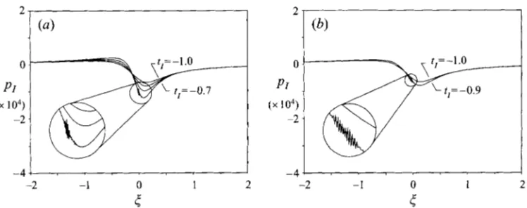
0). In these cases the form of the singularity was essentially similar to that of the terminal solution shown in figure 5 except that the singularity always occurred at an earlier time. For example, singularity times for a few different meshes are given in table 1. These results appeared encouraging since the singularity time found by Peridier et al. (1991b) was approximately TI, = -3.0 (the exact value varied slightly with Reynolds number). As suggested by table 1, however, it subsequently proved impossible to obtain a grid-independent solution; as finer meshes were used, a singularity occurred at progressively earlier times.

As the mesh was refined further, an irregularity appeared in the solution, and results for a typical case are shown in figure 6 which were obtained using a mesh defined by Zo = SOl,JO = 401 and a = 1.0. Before describing the nature of the irregularity, some general features of the solution will be discussed. The position of the upper shear layer

PI

shown in figure 6(a), evolves essentially as in the non-interactive case; the effect of the interaction is small globally. The pressure perturbation PI induced by the growing boundary layer is shown in figure 6(b), where it may be noted that the magnitude is small due to the factor (-tIo)-11/4 in the interaction condition (3.9). Figures 6(c) and 6(d) show the streamwise velocity perturbation and particle position perturbation, respectively, along the centreline

4

= 1, and it is these perturbation quantities which most clearly reveal the overall effects of the interaction. Recall that the streamwise velocity function uI becomes large near the upper and lower shear layers, as well as upstream and downstream of the interaction region. Consequently, the velocity perturbation, which is small in magnitude, only alters the flow appreciably in region I1 in the immediate vicinity of the centre of the domain, near the point

(g,$)

= (0, l), where the terminal-state velocity is small. Recall also that the terminal- state velocity along the central line is positive upstream of ( f , i j ) = (0,l) and negative downstream of this point (cf. figure 2). With this in mind, the perturbation velocity (figure 6c) reveals an increasing positive perturbation just upstream of

g

m 0 and a negative perturbation just downstream of this point. Thus, the interaction accelerates the focusing of the flow toward the eventual separation point at x = x,; this suggests that the onset of the singularity would likewise be accelerated by interaction, which is consistent with the results of the coarse mesh calculations given in table 1.

In figures 6(c) and 6(d) it may be seen that there is an irregularity exhibited in the latter stages of the integration in the form of short-length-scale spikes centred near

g

m 0 which form in the velocity perturbation and particle position perturbation

Unsteady boundary-layer separation 245

15 5

10 0

PI

P I (. 104)

5 -5

0 0

-2 -1 0 1 2 -2 -1 0 1 2

XI

5

8 8

4 4

UI XI-<

(x 104) ( x 105)

0 0

-4 -4

-2 -1 0 1 2 -2 -1 0 1 2

5

5

FIGURE 6. Interactive calculation with a = 1.0. (a) Equation of the upper shear layer

PI.

(b) Induced pressure p I . ( c ) Streamwise velocity perturbation Ur along centreline = 1. (d) Particle position perturbation X I -

5

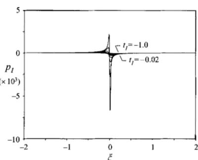
along centreline = 1.

Note that halving the parameter a approximately doubles the number of points in the vicinity of

5

= 0. Comparing the results for the induced pressure in figure 7 with the case shown in figure 6(b), it becomes apparent that as more points are concentrated near

5

= 0, an instability occurs which is manifest at earlier times for finer meshes. This type of behaviour is reminiscent of the short-wavelength instability found by Ryzhov & Smith (1984) in considering dynamic stall and by Tutty & Cowley (1986) for triple-deck-type interactions ; such an instability does not permit grid-independent solutions, because smaller step sizes in the mesh admit shorter-wavelength, faster- growing modes. This also accounts for the occurrence of the instability near

5

= 0, where the step sizes in physical space are smallest due to the transformation (3.23). The possible presence of an instability in the ‘first’ interactive stage is considered further in 96.

The effects of the other solution parameters on the calculated results support the physical existence of a high-frequency instability in the ‘first’ interactive stage. Increasing the number of points 10 in the streamwise mesh was determined to

have the same effect as reducing the stretching parameter a ; the smaller step sizes promote an earlier onset of the instability. The choice of an initial start time affects the spatial resolution, and the selection of ti0 involves a compromise. In general.

the magnitude of tro should be large, but it follows from equations (3.5) t h a t an