Sources
Daniel Smith-Tone1,2
1Department of Mathematics, University of Louisville, Louisville, Kentucky, USA
2National Institute of Standards and Technology, Gaithersburg, Maryland, USA
Abstract. This note was originally written under the name On the Se-curity of HMFEv and was submitted to PQCrypto 2018. The author was informed by the referees of his oversight of an eprint work of the same name by Hashimoto, see eprint article /2017/689/, that completely breaks HMFEv, rendering the result on HMFEv obsolete. Still, the author feels that the technique used here is interesting and that, at least in principal, this method could contribute to future cryptanalysis. Thus, with a change of title indicating the direction in which this work is leading, we present the original work with all of its oversights intact and with minimal cor-rection (only references fixed).
At PQCRYPTO 2017, a new multivariate digital signature based on Multi-HFE and utilizing the vinegar modifier was proposed. The vine-gar modifier increases the Q-rank of the central map, preventing a direct application of the MinRank attack that defeated Multi-HFE. The au-thors were, therefore, confident enough to choose aggressive parameters for the Multi-HFE component of the central map (with vinegar variables fixed). Their analysis indicated that the security of the scheme depends on the sum of the number of variableskover the extension field and the numbervof vinegar variables with the individual values being unimpor-tant as long as they are not “too small.” We analyze the consequences of this choice of parameters and derive some new attacks showing that the parametervmust be chosen with care.
Key words: Multivariate Cryptography, HMFEv, Q-rank
1
Introduction
Note: The attack presented on HMFEv is obsolete, due to the attack by Hashimoto in [1]. The sections relevant to linearization equation extraction are Sections 5 (an original attack on multi-HFE) and 6 (filtering out noise). What follows is the original introduction.
We are currently engaged in a massive international project to secure infor-mation and communication from adversaries with access to large scale quan-tum computers. Since Shor’s algorithm broke public key cryptography in this paradigm, see [2], we have come a long way developing the mathematics of post-quantum cryptography. The science is now sufficiently advanced for us to make educated decisions in how to move forward.
The National Institute of Standards and Technology (NIST) has begun evalu-ating submissions for post-quantum standards with the primary task of securing the internet in the coming quantum age. NIST’s call for proposals, see [3], out-lines the requirements of these technologies and illustrates the criteria by which they are evaluated. The principal prerequisite of any submission is to achieve certain security levels against quantum adversaries.
Multivariate public key cryptography (MPKC) provides a platform for po-tentially achieving these security levels. Multivariate cryptosystems rely on two known NP-complete problems for their hardness. The first is the MQ-problem: the problem of solving systems of nonlinear multivariate equations over a field. The second is the morphism of polynomials (MP) problem: the problem of de-termining whether there is a morphism between two polynomial systems. While typically multivariate cryptosystems lack a complexity theoretic reduction to one of these problems, there is a small collection of cryptanalytic techniques that often can be addressed specifically to derive security results.
In particular, MPKC has produced a few digital signature schemes that have withstood the test of time. Variations on the ideas of HFEv- and UOV, see[4, 5] have been around since the late 1990s without suffering any devestating attacks. PFLASH, see [6], which appeared to many to be weak, has now survived a decade and has fairly strong security arguments, see [7, 8].
Of course, we should not forget the other face of MPKC signatures. Oil-and-Vinegar (OV), SFLASH and Square, see [9–11], to name a few, were soundly defeated in [12–14]. Yet sometimes out of the ashes rises a new and more powerful scheme. The idea for UOV came from the attack on OV, and PFLASH is the progeny of SFLASH.
In this manuscript, we analyze a possible such phoenix. Multi-HFE, first proposed in [15], was completely broken in [16] by a clever MinRank attack exploiting the extremely low Q-rank of the central map of multi-HFE. The idea was breathed new life recently at PQCRYPTO 2017 in [17] where the idea of using the vinegar modifier on multi-HFE as a patch for the low Q-rank was proposed.
We offer a more precise justification for these claims by developing an ex-plicit attack to filter out the vinegar variables when too few are included in the construction. The attack is statistical, bootstrapping an original attack on multi-HFE to form a distinguisher that successfully discerns whether a map is random or of multi-HFE shape. The attack depends on a disparity in the distribution of cubic forms generated from HMFEv instances with differing numbers of vinegar variables added. As the number of vinegar variables is increased, the distance between the distributions is decreased so that the addition of sufficiently many vinegar variables renders the attack impotent, thus demonstrating the need for a large number of vinegar variables.
The paper is organized as follows. In the next section, we describe the multi-HFE and HMFEv constructions. The following section describes Q-rank, an essential notion for understanding modern multivariate cryptography. In section 4, we review the previous cryptanalyses of multi-HFE and HMFEv. The subse-quent section contains an original cryptanalysis of multi-HFE. Then, in Section 6, we extend this method into an attack filtering out the vinegar variables from HMFEv. Finally, we conclude, noting the affect these results have on parameter selection for HMFEv.
2
HFE Variants
Multivariate public key schemes can be broadly categorized as either “small field” or “big field” schemes. Small field schemes rely on the structure of a single field for their construction whereas the big field schemes rely on the multplicative structure of a hidden extension field. Given an extension E of F = GF(q) of degreel, one can see that any monomial inE[X] of the formXqa+qb
is the product of two Frobenius automorphisms, that is the product of twoF-linear functions. Therefore, this monomial can be written as a vector of quadratic functions over F; hence, we call such a monomial F-quadratic. Big field multivariate schemes are based on easily invertibleF-quadratic maps fromEto Ewith the structure hidden by an isomorphism of polynomials.
Definition 1 Two vector-valued multivariate polynomials F andGare said to be isomorphicif there exist two affine mapsT, U such that G=T ◦F◦U.
The following diagram summarizes the above discussion in the case of multi-HFE. One thing to note is that a multivariate polynomial ring over the extension is used instead of an univariate polynomial ring.
Ek f //
Ek
(φ−1)k
Fn U //Fn F // (φ)k
OO
2.1 Multi-HFE
The HMFEv digital signature scheme of [17] is based on the multi-HFE prim-itive originally specified in [15]. Recalling the construction of multi-HFE, we choose a finite fieldF, a degree `extension E, and an integerk. Settingn=k`
as the number of variables, one constructs n polynomials in F[x1, . . . , xn] as follows. Select an F-vector space isomorphism φ : F` →
E and two affine iso-morphisms T, U : Fk` →Fk`. Select the quadratic mapf = (f1, . . . , fk) where
fi(X1, . . . , Xk)∈E[X] is defined by
fi(X) =
X
1≤r,s≤k
αi,r,sXrXs+
X
1≤r≤k
βi,rXr+γi,
for 1≤i≤k. One then composes these maps producing the public key
P(x1, . . . , xn) =T◦(φ−1)k◦f ◦(φ)k◦U, where (φ)k=φ×φ× · · · ×φwithkcoordinates.
A signature is the preimage of a certificate and so verification is accomplished by evaluating the public key at the signature value. The signature is generated by inverting each of the maps. The inversion off is accomplished by generating a univariate polynomial, for example with a Gr¨obner basis algorithm with an elimination ordering, solving for a single variable and then repeating.
2.2 HMFEv
The modification of multi-HFE producing HMFEv is to add v additional vari-ables and augment the definitions ofβi,r andγi. Specifically, we letU :Fk`+v→ Fk`+v andT :Fk`→Fk` be affine isomorphisms and define the quadratic map
f = (f1, . . . , fk) by
fi(X) =
X
1≤r,s≤k
αi,r,sXrXs+
X
1≤r≤k
βi,r(xn+1, . . . , xn+v)Xr+γi(xn+1, . . . , xn+v),
for 1≤i≤kwhereβi,r:Fv→Eandγi:Fv →Eare linear forms in the vinegar variablesxn+1, . . . , xn+v. The public key is given by
P(x1, . . . , xn+v) =T◦(φ−1)k◦f◦[(φ)k×idv]◦U.
A signature is the preimage of a certificate and so verification is accom-plished by evaluating the public key at the signature value. Signature generation is accomplished by randomly selecting values for the vinegar variables, which collapses f into the central map of a multi-HFE scheme. Then one inverts P
3
Q-Rank
As with all of the schemes in the HFE lineage, Q-rank plays an important role in the cryptanalysis of multi-HFE. Adapting the definition to multivariate ex-tension field maps we may write the following definition.
Definition 2 The Q-rank of any quadratic map f(x) on Fk`
q with respect to the degree ` extension E is the rank of the quadratic form (φ−1)k◦f ◦(φ)k in K[X0, . . . , Xk`−1] via the identification X`(n−1)+i =φ(πn(x))q
i
, where 1≤n≤
k,0≤i < `andπn is the projection on to nth group of` coordinates ofx. Note that in the case of multi-HFE, the total degree of the central map over Eis two. Therefore, the Q-rank is bounded bykin all instances.
It is also important to note that although Q-rank is not preserved by isomor-phisms of polynomials, the min-Q-rank in the linear span of f is preserved by such isomorphisms. This quantity is what is relevant for cryptography, and this is the property that has led to the attacks on multi-HFE.
4
Previous Cryptanalysis of multi-HFE and HMFEv
Being derived from multi-HFE, which is well known to have been broken, we review the security analysis of HMFEv and the cryptanalyses of muli-HFE. We offer an original, but trivial, extension to the security analysis of [17] which fits well in this section.
4.1 Cryptanalyses of Multi-HFE
Multi-HFE has been cryptanalyzed in a couple of related ways. In [16], the low Q-rank property described in Section 3 is exploited. Specifically, one may construct the rankk` representationΦ:Ek→
Adefined by
Φ(α, β, . . . , γ) = (α, αq, . . . , α`−1, β, βq, . . . , β`−1, . . . , γ, γq, . . . , γ`−1).
Since each component of the central map f : Ek → Ek is of total degree two, represented as a quadratic form overAit can involve onlykcoordinates, that is, the coordinates of α, β, . . . , γ above. Therefore, each coordinate of the central map has Q-rank at mostk.
Since multi-HFE is typically presented withk = 2 or k = 3, which means that the Q-rank of the central map is at most 3, the scheme is quite vulnerable to a MinRank attack via minors modeling, which is exactly what was efficiently done in [16]. To perform the attack, the sum of the product of variablesti and the matrix representations of the public quadratic forms is constructed. By the Q-rank property, this matrix has rank at most 3. So by collecting all of the 4×4 minors, one generates an ideal whose Gr¨obner basis can be computed overFand whose variety is then computed overE.
4.2 Previous Security Analysis of HMFEv
In [17], a preliminary analysis of HMFEv is presented. The authors consider the two principal attacks that seem relevant to the new scheme: the minrank attack and the direct algebraic attack.
For the MinRank attack, they note that the as long as v ≤ ` the vinegar variables can be modelled by another variable over the extension field, where it is easy to show that the Q-rank of the central map is bounded by k+v. Experiments support the claim that this bound is tight, so they conclude that the complexity of the MinRank attack on HMFEv is O(`(k+v+1)ω).
We can verify this claim analytically for allv in the following manner. For simplicity we consider the odd characteristic case. The argument is similar for characteristic two.
Proposition 1 The min-Q-rank of an HMFEv public key with parameters `,k
andv isk+v. Proof. Letφ:F` →
E be a vector space isomorphism. Choose a representation
ψ :Ek →
Adefined by ψ(X1, X2, . . . , Xk) = (X1, X q 1, . . . , X
q`−1
1 , X2, . . . , X q`
k ). We then construct the vector space isomorphismΦ:Fk`+v →
A×Fv defined by
Φ= (ψ×idv)◦(φk×idv).
We may now express the coordinates of the central map overEas quadratic forms overA×Fv. We observe that, due to the degree bound of two in the multi-HFE component, each coordinatefi of the central mapf satisfies fi =Qi◦Φ, whereQi is a quadratic form on A×Fv with the following shape
Qi=
0 0· · · 0αi120· · · 0αi1k0· · · 0βi11· · · βi1v 0 0· · · 0 0 0· · · 0 0 0· · · 0 0 · · · 0 ..
. ... . .. ... ... ... . .. ... ... ... . .. ... ... . .. ... 0 0· · · 0 0 0· · · 0 0 0· · · 0 0 · · · 0
αi120· · · 0 0 0· · · 0αi2k0· · · 0βi21· · · βi2v 0 0· · · 0 0 0· · · 0 0 0· · · 0 0 · · · 0 ..
. ... . .. ... ... ... . .. ... ... ... . .. ... ... . .. ... 0 0· · · 0 0 0· · · 0 0 0· · · 0 0 · · · 0
αi1k 0· · · 0αi2k 0· · · 0 0 0· · · 0βik1· · · βikv 0 0· · · 0 0 0· · · 0 0 0· · · 0 0 · · · 0 ..
. ... . .. ... ... ... . .. ... ... ... . .. ... ... . .. ... 0 0· · · 0 0 0· · · 0 0 0· · · 0 0 · · · 0
βi11 0· · · 0βi21 0· · · 0 βik10· · · 0 γi11 · · · γi1v
βi12 0· · · 0βi22 0· · · 0 βik20· · · 0 γi12 · · · γi2v ..
. ... . .. ... ... ... . .. ... ... ... . .. ... ... . .. ...
βi1v 0· · · 0βi2v 0· · · 0βikv0· · · 0 γi12 · · · γivv
,
quadraticsγirsxn+rxn+s. Thus the Q-rank off, which is bounded by the Q-rank offi for 1≤i≤k is bounded byk+v. It is easy to see that in probability it is exactly k+v.
Addressing the complexity of the algebraic attack on HMFEv, the authors assume the tightness of the bounds given in both [17, Theorem 3] and in [19, Theorem 3.1] to conclude that the degree of regularity of the HMFEv system is
dreg≤
(
(q−1)jk+v2 k+ 2 ifqis even, and q−1
2 (k+v) + 2 otherwise.
Again, this claim is supported by experiments showing that the above bound is fairly tight. They noted specifically that the choice of k and v were irrele-vant as long as they were not too small, indicating in [20] that k, v ≥ 2 suf-fices. Using these estimates they conclude the complexity of the direct attack is O n+dreg
dreg
2 n 2
.
5
A New Attack on Multi-HFE
Multi-HFE has a couple of successful cryptanalyses as mentioned in the previous section. In both [16] and [18], a full key recovery attack is developed. We now introduce a less sophisticated attack focusing on the choice of central map of HMFEv which produces a kth-root speed-up in preimage search. As we will soon see, this technique allows information to be filtered through the vinegar modifier when an insufficient number of vinegar variables is used.
We consider the characteristic two case with k = 3. Since any multi-HFE instance over the fieldFq whereqis even can be equivalently defined overGF(2), we consider the case in whichq= 2. LetEbe the degree`extension over which the central multi-HFE map of HMFEv is given by
Y1=X1X2+α1,1X1+α1,2X2+α1.3X3+α1,4
Y2=X2X3+α2,1X1+α2,2X2+α2.3X3+α2,4
Y3=X1X3+α3,1X1+α3,2X2+α3.3X3.+α3,4
(1)
Consider the graded ring (Ad) =E[X1, X2, X3]/I, graded by total degree, where
Iis the ideal generated by the homogeneous quadratic components of the above three polynomials. It is clear that dimE(Ad) = 3 if d >0 and is one if d= 0. Therefore the Hilbert Series ofIis
HSI(t) = 1 + 2t
1−t ,
It is easy to see that the polynomialsYiin Equation (1) inherit this relation. To be explicit, we compute
X3Y1+X1Y2=α1,1X1X3+α1,2X2X3+α1,3X32 +α2,1X12+α2,2X1X2+α2,3X1X3 +α1,4X3+α2,4X1
=α1,1Y3+α1,2Y2+α1,3L(X3) +α2,1L(X1) +α2,2Y1+α2,3Y3 +α1,2(α2,1X1+α2,2X2+α2.3X3) +α2,1(α1,1X1+α1,2X2+α1.3X3) +α2,3(α3,1X1+α3,2X2+α3.3X3) +α1,4X3+α2,4X1,
(2)
which is GF(2)-affine in both X and Y. Another linearly independent such relation can be derived from X3Y1 +X2Y3; however, the remaining relation
X1Y2+X2Y3is the sum of the first two relations.
It is easy to extend this analysis to anyk≤5, see Appendix A. Fork >5 it is still possible to recover relations betweenX andY linear inX; however, they must in general be nonlinear in Y.
Passing these relations toGF(2) and generalizing to k, we obtain (k−1)`
linearly independent relations linear in bothxandy. Composing with the affine transformationsU andT−1, we obtain (k−1)`linearization equations(orhigher order linearization equations if k > 5) on the multi-HFE instance. Thus we obtain a decryption oracle with runtimeO(2`), performing a preimage search on a space of onekth the dimension of the signature space.
6
Distilling Vinegar
The existence of the linearization equations of the previous section function as a criterion for the image of a linear projection being orthogonal to the vinegar subspace. From this idea, we build a distinguisher acting on projected HMFEv keys of the formP◦π, able to determine whether a subspace of the vinegar space is orthogonal to Im(π). We then bootstrap this technique to a key recovery. For the simplicity of avoiding the higher dimensional tensors necessary in the analysis of the higher order linearization equations case, we restrict to the case thatk≤5 guaranteeing (k−1)`linearization equations, noting that the general theory works analogously.
6.1 Filtering Vinegar Variables
forms can be as much as (k−1)`smaller than for random projections if rank(π) is sufficiently large. To make this clear, we review the theory of linear embeddings of homogeneous forms on a vector space.
Theorem 1 Let V be an n-dimensionalF-vector space. LetF[X]d be the space of homogeneous polynomials of degree d on V and let π : V → V be a rank r
projection. The rank of the linear map Tπ :F[X]d→F[X]d defined byTπ(f) =
f◦π is r+dd−1if |F| ≥d.
Proof. We show thatTπ(f) is in the span of r+dd−1d-tensors. In particular, we may without loss of generality assume thatπ projects onto the firstrstandard basis vectors ofV, so thatTπ(f) involves onlyrvariables. Since there are exactly
r+d−1 d
distinct degreedmonomials inrvariables, the rank ofTπ(f) is r+dd−1
. We note that when |F| < d that some of the monomials in Theorem 1 are equivalent to smaller degree monomials, and thus such homogeneous forms of degreedare degenerate and the rank in this sense is smaller. A particular case to note is that of cubic forms overGF(2). The number of such monomials in this case with distinct values is r3
+ r2
+ r1
due to the fact that x2
i =xi. Thus, forGF(2), we obtain a rank bound of r3
+ r2
+ r1
=r3+5r 6 .
Corollary 1 Let V be an n dimensional F-vector space. Letg : V → V be a quadratic map. For any rankrprojectionπ:V →V, the rank of the linear map
Tg,π : F[X]2 → F[X]3 defined by Tg,π(f)(x) = hπ(x)A, g(π(x))i, where f(x) = hxA, xi is the inner product representation of f, is at most min{r3+5r
6 , rn} if |F|= 2and at most min{ r+23
, rn} otherwise.
Proof. First note that sinceπis composed with the matrix representingf, there are only actually rn degrees of freedom in choosing f. We therefore focus on establishing the bound when ris sufficiently low.
Clearly we may write Tg,π =Tπ◦Tg where Tg : F[X]2 → F[X]3 is defined by Tg(f)(x) = hxA, g(x)i. Since the rank of Tπ has the appropriate bound by Theorem 1, the only thing to show is thatTg is linear. ThatTg(ap) =aTg(p) is obvious. Letp, q∈F[X]2 and letAp andAq be the matrix representations ofp andq, respectively. First,
(p+q)(x) =p(x) +q(x) =hxAp, xi+hxAq, xi=hx(Ap+Aq), xi. Then we obtain
Theorem 2 Let P be a public key of HM F E with parametersq= 2,k,` and
v. Let π be the rank r≤n=k` projection orthogonal to the vinegar subspace. Then
Rank(TP,π)≤min
r3+ 5r
6 , rn−(k−1)`
.
Proof. We may calculate the rank ofTP,πdirectly by specifying a quadratic form
f ∈ F[X]2 by its matrix representation A = (aij) and directly computing the nullity ofTP,π. Recall that due toπwe may considerAto have anr×nblock of possibly nonzero values. Notice that by the previous section, there are (k−1)`
linearization equations; therefore, wheneverrn−r3+5r
6 <(k−1)`, we know that the kernel ofTP,πis at least
(k−1)`+r3+5r6 −rn-dimensional. Thus the rank ofTP,π is at most r
3+5r
6 when this quantity is less than rn−(k−1)`, and is at mostrn−(k−1)`otherwise.
Restricting the codomain ofTP,π to the image ofTπ, we can see that if the rank of TP,π is less than min
n
r3+5r
6 , rn−(k−1)`
o
, then there is a nontrivial cokernel, which is to say that there are additional linearization equations. For random functions one should expect this event to occur with low probability. Un-surprisingly, there is a distinction in the behavior of a multi-HFE primitive and a random function under the vinegar modification in this respect. Furthermore, there is a noticable relationship between the rank of TP,π and the dimension of the intersection of the dual of the cokernel ofπand the vinegar subspace,Vvin, as illustrated in Table 1.
r
α
d
0 1 2 3 4
β
1 2 3 4 5 6 7 8 9 10 11 12
1 3 7 14 25 41 63 92 108 120 132 144
13.99 24.95 40.95 62.80 91.64 108 120 132 144 7 13.96 24.97 40.89 62.82 91.5 108 120 132 144 2.99 7 13.97 24.91 40.78 62.52 91.02 108 120 132 144 1 2.99 6.98 13.96 24.86 40.51 62.3 89.81 107.44 119.83 131.87 143.88 1 2.99 6.9 13.85 24.63 40.32 61.2 84.91 99.76 111.99 124 136
1 3 7 14 25 41 63 88 100 112 124 136
Table 1. Average rank of TP,π over 100 trial runs where the rank of π is r and dim(coKer(π)∗∩Vvin) =dforn= 12 andv= 4. For comparison, we also include the valuesα= min{r3+5r
6 , rn}andβ= min{
r3+5r
6 , rn−(k−1)`}.
Notice, in particular, that the data in columnsr= 7 and 8 of Table 1 exhibit a larger range of values among rows d = 0 through d= 3 than the remaining columns. The reason is that for these values ofr, the image ofTπis approaching
This transition appears to grow sharper asdim(coKer(π)∗∩Vvin) approaches
dim(Vvin). Apparently, the symmetries in the multi-HFE structure skew the distribution of Rank(TP,π) away from that of Rank(Tf,π) for a random function
f and the degrees of freedom of the values of the vinegar variables in the image of πis a metric for passing between these two extremes. The disparity is more apparent with fewer vinegar variables, see Table 2.
Remark 1 The variance of the data increases nearr=√6n−5; however, the variance is still small, is even smaller with larger qand is extremely small with
d= 0 in all cases.
r
α
d
0 1 2
β
1 2 3 4 5 6 7 8 9 10 11 12
1 3 7 14 25 41 63 92 108 120 132 144
2.99 6.95 13.92 24.92 40.86 62.49 91.07 108 120 132 144 1 3 6.97 3.9 24.72 40.63 62.25 89.7 107.21 119.55 131.57 143.67 0.98 2.97 6.95 13.84 24.73 40.04 6.36 84.95 99.72 112 124 136
1 3 7 14 25 41 63 88 100 112 124 136
Table 2. Average rank of TP,π over 100 trial runs where the rank of π is r and dim(coKer(π)∗∩Vvin) =dforn= 12 andv= 2. For comparison, we also include the valuesα= min{r3+5r
6 , rn}andβ= min{
r3+5r
6 , rn−(k−1)`}.
6.2 Key Recovery
The method for turning this statistical anomaly into a key recovery is as follows. First one randomly generates a large number of rankr≈√6n−5 projectionsπ
and selects a cutoff rankR for TP,π. For any π, if the rank ofTP,π is bounded byR, πis placed in a database. Next one chooses a numbers of coKer(π)∗ to intersect in the hopes of filtering out a vector v in Vvin. Success is measurable immediately by estimating the distribution of Rank(TP0,π) near r =
√ 6n−5, whereP0isP composed with the projection onto the orthogonal complement of
v. Finally, one repeats this process, which becomes easier asv diminishes. For this method to be effective, one must fine tuneRandsto minimize the number of low rank TP,π required to be computed. To estimate the optimal s we note that the probability of a vector lying in the intersection ofs subspaces of dimension r in a vector space of dimensionn+v is roughly qsr−(s−1)(n+v). Similarly, under the assumption that each of theksubspaces has ad-dimensional intersection with a fixed v-dimensional subspace, the probability that a vector in this subspace lies in the intersection is roughlyqsd−(s−1)v. When these prob-abilities are equal, i.e. when s ≈ n
n+d−r, essentially all of the vectors in the intersection should lie in the fixedv-dimensional subspace. Specifically, whenn
Under the assumption that an R can be found such that the fraction of π
satisfying dim(coKer(π)∗∩Vvin) = d among all π for which the rank of TP,π is bounded by R is significant, the recovery of a vector v ∈ Vvin requires ap-proximatelyqd(r−s)+v(s−1)calculations of the rank ofT
P,π plus some additional linear algebra steps. Thus the complexity of recovering the vinegar subspace is O (rn)ωqd(r−s)+v(s−1)
. Since r ≈ √6n−5, this attack is subexponential in
n for any fixed v. For the special case of v = 2, addressing the claim in [17], we have d= 1 and s= 2 for sufficiently large n and this formula simplifies to O (rn)ωqr+1
=On3ω/2q√6n−5+1.
Experiments show that this method is effective in practice on small scale schemes. In the case of q = 2, l = 4, k = 3 and v = 2, only four rank 9 projections πsatisfying rank(TP,π)≤R = 107 were needed to find a vector in
Vvin. On average one in 384 projectionsπsatisfied this property, supporting the above complexity estimate.
It is interesting to note that the cutoff phenomenon in the rank of TP,π, though present, is not extremely sharp, at least when r ≈√6n−5; therefore, for small values ofva value ofRcan be found to make the attack effective. Still, for v >4, we estimate that the cutoff is sharp enough that one would require
d >1 to find a suitable value ofR; however, this would render the attack worse than brute force for essentially any parameters, due to the largeqof HMFEv.
7
Other Techniques
In [21], new statistical methods for attacking HFEv- are advanced. In principle, the attacks are applicable to HMFEv as well; however the complexity analysis is not the same. Similar to the attack presented in Section 6, these techniques incorporate projections and the calculation of invariants to bootstrap a distin-guisher to a key recovery attack, though the approaches are different.
The first approach combines projection with the MinRank method. There are two possible variants of this technique: Project-then-MinRank and MinRank-then-Project. The Project-then-MinRank strategy works by noting that there is a distinction in the Q-rank of the central map under a projection reducing the dimension of the vinegar subspace versus a projection that is full rank when restricted to the vinegar subspace. Both attacks, however, still require the Min-Rank step to be executed. In the context of HMFEv, as long ask+v is large, even a random reduction in the rank of two or three, which occurs with very low probability, will not reduce the complexity sufficiently to risk the integrity of the scheme. Due to the relatively large size ofqin the proposed parameters of HMFEv, the MinRank-then-Project method seems to be the more efficient. In this case the complexity of the MinRank-then-Project approach is dominated by the cost of the MinRank step, which has complexityO `(k+v+1)ω
, as predicted in Section 4.2.
degree of regularity dbut random systems of smaller dimension have degree of regularity d−1. Because of the low Q-rank property of HFE, there is a higher probability that projected systems from an HFE instance will have a lower degree of regularity. The idea is that if the projection eliminates a vinegar variable it may be detectable in the degree of regularity of the projected scheme.
The complexity of this attack in application to HMFEv is also dependent on the sum k+v. The projection must have a large enough corank to have a sufficiently high probability of achieving a reduction in the degree of regularity and when a vector in the vinegar subspace is found, there is no additional infor-mation about the basis of the vinegar subspace revealed. Thus the attack must be repeated with the slight advantage of one additional equation specifying a one-dimensional subspace of the subsequent kernel.
The complexity of the entire attack is approximatelyOqn−t n+v+d d
2 n+v 2
, wheretis the co-dimension of projection optimal for distinguishing anddis the degree of regularity at which distinguishing occurs. The quantitytis a decreas-ing function ofk+v. This fact along with the size ofqmake this new technique infeasible for the parameters suggested in [17].
8
Experiments
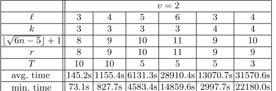
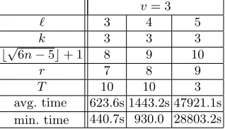
We ran a series of experiments with Magma1, see [22], on a 3.2 GHz Intel® XeonCPU, testing the first step of the attack, recovering a vector in the vine-gar subspace, for a variety of values of`withv= 2 orv= 3 andk= 3 ork= 4. Tables 3 and 4 summarize some of our results in thev= 2 andv= 3 cases, re-spectively. The data support our complexity estimate ofO (rn)ωqd(r−s)+v(s−1)
.
v= 2
` 3 4 5 6 3 4
k 3 3 3 3 4 4
b√6n−5c+ 1 8 9 10 11 9 10
r 8 9 10 11 9 9
T 10 10 5 5 5 3
avg. time 145.2s 1155.4s 6131.3s 28910.4s 13070.7s 31570.6s min. time 73.1s 827.7s 4583.4s 14859.6s 2997.7s 22180.0s
Table 3.Average time (in s) forT instances of the vinegar recovery attack of Section 6 on HMFEv(q= 2, k, `, v= 2) for various values of`andk.
There is an interesting artifact in the data that should be pointed out explic-itly. For almost all of the parameters tested, the value of nis too small for our estimate ofsto achieve an upper bound of 2. That is, the number of coKer(π)∗
1
one must intersect in order to essentially guarantee that a nontrivial intersec-tion will reveal a vector in Vvin is, for most of these low values of n, greater than 2. Therefore, for these small tests, it is likely that we will see nonempty intersections constructed from two projections revealing a vector not contained in Vvin. Still, we found it more efficient for these small scale experiments to choose a value ofs= 2. In nearly every experiment, we found nonempty inter-sections which did not intersect the Vvin. In fact, aside from a couple of lucky instances far from the mean, there was exactly one set of parameters for which the nonempty intersectionsalways were inVvin. That test was fork=`= 4, for which our estimate forsis
s= n
n+d−r =
16
16 + 1−9 = 2.
Thus, the tests behave exactly as predicted in the analysis of Section 6.
v= 3
` 3 4 5
k 3 3 3
b√6n−5c+ 1 8 9 10
r 7 8 9
T 10 10 3
avg. time 623.6s 1443.2s 47921.1s min. time 440.7s 930.0 28803.2s
Table 4.Average time (in s) forT instances of the vinegar recovery attack of Section 6 on HMFEv(q= 2, k= 3, `, v= 3) for various values of`.
9
Conclusion
We have demonstrated that the security of HMFEv is not symmetrically depen-dent upon the values k, the number of multi-HFE variables over the extension field, andv, the number of vinegar variables. Due to the extremely low Q-rank structure of multi-HFE, symmetries in the multi-HFE map can percolate through the noise added by the vinegar variables and affect the rank of tensors derived from the public key when there are very few vinegar variables. Thus HMFEv really requires a large number of vinegar variables.
References
1. Hashimoto, Y.: On the security of hmfev. IACR Cryptology ePrint Archive2017
(2017) 689
2. Shor, P.W.: Polynomial-time algorithms for prime factorization and discrete loga-rithms on a quantum computer. SIAM J. Sci. Stat. Comp.26, 1484(1997) 3. Group, C.T.: Submission requirements and evaluation criteria for the
post-quantum cryptography standardization process. NIST CSRC (2016) http://csrc.nist.gov/groups/ST/post-quantum-crypto/documents/call-for-proposals-final-dec-2016.pdf.
4. Patarin, J.: Hidden Fields Equations (HFE) and Isomorphisms of Polynomials (IP): Two New Families of Asymmetric Algorithms. In: EUROCRYPT. (1996) 33–48
5. Kipnis, A., Patarin, J., Goubin, L.: Unbalanced oil and vinegar signature schemes. EUROCRYPT 1999. LNCS1592(1999) 206–222
6. Ding, J., Dubois, V., Yang, B.Y., Chen, C.H.O., Cheng, C.M.: Could SFLASH be Repaired? In Aceto, L., Damg˚ard, I., Goldberg, L.A., Halld´orsson, M.M., Ing´olfsd´ottir, A., Walukiewicz, I., eds.: ICALP (2). Volume 5126 of Lecture Notes in Computer Science., Springer (2008) 691–701
7. Chen, M.S., Yang, B.Y., Smith-Tone, D.: Pflash - secure asymmet-ric signatures on smart cards. Lightweight Cryptography Workshop 2015 (2015) http://csrc.nist.gov/groups/ST/lwc-workshop2015/papers/session3-smith-tone-paper.pdf.
8. Cartor, R., Smith-Tone, D.: An updated security analysis of PFLASH. [23] 241–254 9. Patarin, J.: The oil and vinegar algorithm for signatures. Presented at the Dagstuhl
Workshop on Cryptography (1997)
10. Patarin, J., Courtois, N., Goubin, L.: Flash, a fast multivariate signature algorithm. CT-RSA 2001, LNCS2020(2001) 297–307
11. Clough, C., Baena, J., Ding, J., Yang, B.Y., Chen, M.S.: Square, a New Multi-variate Encryption Scheme. In Fischlin, M., ed.: CT-RSA. Volume 5473 of Lecture Notes in Computer Science., Springer (2009) 252–264
12. Shamir, A., Kipnis, A.: Cryptanalysis of the oil & vinegar signature scheme. CRYPTO 1998. LNCS1462(1998) 257–266
13. Dubois, V., Fouque, P.A., Shamir, A., Stern, J.: Practical Cryptanalysis of SFLASH. In Menezes, A., ed.: CRYPTO. Volume 4622 of Lecture Notes in Com-puter Science., Springer (2007) 1–12
14. Billet, O., Macario-Rat, G.: Cryptanalysis of the square cryptosystems. ASI-ACRYPT 2009, LNCS5912(2009) 451–486
15. Chen, C.O., Chen, M., Ding, J., Werner, F., Yang, B.: Odd-char multivariate hidden field equations. IACR Cryptology ePrint Archive2008(2008) 543 16. Bettale, L., Faug`ere, J., Perret, L.: Cryptanalysis of HFE, multi-HFE and variants
for odd and even characteristic. Des. Codes Cryptography69(2013) 1–52 17. Petzoldt, A., Chen, M., Ding, J., Yang, B.: Hmfev - an efficient multivariate
signature scheme. [23] 205–223
18. Hashimoto, Y.: Cryptanalysis of multi-hfe. IACR Cryptology ePrint Archive2015
(2015) 1160
20. Petzoldt, A., Chen, M.S., Ding, J., Yang, B.Y.: Hmfev - an efficient multivariate signature scheme. Presentation - Post-Quantum Cryp-tography - 8th International Conference on Post-Quantum Cryptogra-phy, PQCrypto 2017, Utrecht, Netherlands, June 26-28, 2017 (2017) https://2017.pqcrypto.org/conference/slides/mqI/HMFEv.pdf.
21. Ding, J., Perlner, R., Petzoldt, A., Smith-Tone, D.: Improved cryptanalysis of hfev-via projection. In Current Submission (2017)
22. Bosma, W., Cannon, J., Playoust, C.: The Magma algebra system. I. The user language. J. Symbolic Comput. 24 (1997) 235–265 Computational algebra and number theory (London, 1993).
23. Lange, T., Takagi, T., eds.: Post-Quantum Cryptography - 8th International Work-shop, PQCrypto 2017, Utrecht, The Netherlands, June 26-28, 2017, Proceedings. Volume 10346 of Lecture Notes in Computer Science., Springer (2017)
A
Existence of Linearization Equations
Theorem 3 Let 3≤k≤5and fori∈ {1, . . . , k} let
Yi =XiXi+1+αi,1X1+· · ·+αi,kXk+αi,k+1,
be a multi-HFE central map over E, where the indices are computed as least positive residues modulo k. Then there exists an E-bilinear relation between Yi andXi.
Proof. Consider the variableXi for 1≤i≤k. There are two nontrivial syzygies given by LT(XiYi+1)−LT(Xi+2Yi) and LT(XiYi−2)−LT(Xi−2Yi−1) involving
Xi. One can clearly see that summing overiwe obtain exactlyk syzygies since every one is counted exactly twice. The case ofk= 3 is the exceptional case in which the span of these syzygies is less than k-dimensional; however, we have already seen that the result holds fork= 3.
The non-leading terms ofXiYi+1 are either linear inX, specifically, αiiXi2; linear in X and Y, i.e. of the form XiXi±1 = Y(i±1−1)/2+Pj6=i±1αjXj; or quadratic inX, such asXiXswheres6∈ {i−1, i, i+ 1}. There are exactly k
2−3k
2 quadratics XiXj with j 6∈ {i−1, i, i+ 1}. Each such term can be eliminated with linear combinations ofXiYi+1−Xi+2Yiprovided k
2−3k
2 ≤k, which occurs ifk≤5.
B
Toy Example
B.1 The Public Key
We construct the degree`extensionE=F2(b) whereb2+b+ 1 = 0. We specify the canonical isomorphism φ : F2
2 → E. We randomly fix the central map F, specifying its coordinates,
Y1=X1X2+φ(L11(XV))X1+φ(L12(XV))X2+φ(L13(XV))X3+φ(x27, x7x8)
Y2=X2X3+φ(L21(XV))X1+φ(L22(XV))X2+φ(L23(XV))X3+φ(x7x8, x27+x 2 8)
Y3=X1X3+φ(L31(XV))X1+φ(L32(XV))X2+φ(L33(XV))X3,+φ(x28, x7x8)
where
L11=XV
1 1 1 1 1 1 1 1 0 0 1 1
,L12=XV
0 1 1 1 0 1 0 0 1 1 1 1
,L13=XV
0 0 0 1 0 0 1 0 1 1 0 0
,
L21=XV
0 0 0 1 1 0 1 0 0 0 1 1
,L22=XV
1 1 0 1 1 1 0 1 1 0 0 0
,L23=XV
0 1 0 0 1 1 1 1 1 0 1 1
,
L31=XV
1 0 0 1 1 0 1 0 1 1 0 1
,L32=XV
1 1 1 0 0 1 1 0 1 0 0 0
, L33=XV
1 0 0 1 1 0 0 1 0 0 1 0
,
and two invertible linear transformationsT andU:
T =
0 0 0 0 1 0 1 0 0 1 1 1 0 1 0 1 1 1 1 1 0 0 0 1 1 1 1 1 0 0 0 0 0 1 1 0
, andU =
1 0 0 1 0 0 0 0 1 1 1 0 0 1 0 0 1 1 0 1 0 0 0 0 0 0 0 1 0 0 0 0 1 1 0 1 1 1 0 0 0 0 1 1 0 0 0 0 0 0 0 0 0 0 0 1 0 0 0 0 0 0 1 1
.
ComposingP =T◦φ−1◦F◦(φ×id
V)◦U, we obtain the public key expressed here in polar form overF2:
P0=
1 1 1 1 0 1 1 1 1 1 1 1 0 1 1 1 1 1 0 0 0 1 0 0 1 1 0 0 0 0 1 1 0 0 0 0 0 0 1 0 1 1 1 0 0 0 1 0 1 1 0 1 1 1 0 1 1 1 0 1 0 0 1 1
,P1=
0 0 0 0 0 0 0 1 0 0 1 0 1 1 1 1 0 1 0 0 1 0 1 0 0 0 0 0 1 0 0 0 0 1 1 1 1 1 1 0 0 1 0 0 1 0 0 1 0 1 1 0 1 0 0 1 1 1 0 0 0 1 1 1
,P2=
0 0 0 0 1 0 1 1 0 1 1 0 1 0 1 1 0 1 0 0 0 0 1 1 0 0 0 0 0 0 0 1 1 1 0 0 0 0 0 1 0 0 0 0 0 0 1 1 1 1 1 0 0 1 1 1 1 1 1 1 1 1 1 1
,
P3=
1 0 1 1 0 1 1 0 0 0 1 1 1 0 1 0 1 1 0 0 0 1 0 0 1 1 0 0 1 0 0 1 0 1 0 1 0 1 0 1 1 0 1 0 1 0 1 0 1 1 0 0 0 1 1 0 0 0 0 1 1 0 0 1
,P4=
1 0 0 1 0 0 1 0 0 0 0 0 0 0 0 1 0 0 1 1 0 1 1 0 1 0 1 0 0 0 0 1 0 0 0 0 1 1 1 0 0 0 1 0 1 0 0 0 1 0 1 0 1 0 0 1 0 1 0 1 0 0 1 1
,P5=
1 0 1 1 0 1 0 1 0 0 1 0 1 0 0 0 1 1 0 0 1 1 1 0 1 0 0 0 1 0 0 0 0 1 1 1 1 0 1 1 1 0 1 0 0 0 1 0 0 0 1 0 1 1 1 1 1 0 0 0 1 0 1 0
.
B.2 Recovering the Vinegar Subspace
We choose random rank r= 5 projectionsπand compute the rank of
TP,π(x) =π(x)
t1,1· · · t1,6 ..
. . .. ...
t5,1· · · t5,6
y
>,
where P(π(x)) =y. Setting a rank bound of 19, we generate mapsπsatisfying rank(TP,π)≤19. As we find solutions,πi we compute coKer(πi)∗∩coKer(πj)∗.
In this experiment, the first two projections π1 and π2 satisfying the rank bound are
Π1=
1 1 1 1 0 1 0 0 0 0 1 0 1 0 1 1 0 1 0 1 1 1 1 1 0 0 0 1 0 0 1 1 0 0 0 0 0 0 1 1
andΠ2=
1 0 0 0 1 0 0 0 0 1 1 0 0 1 0 0 0 1 1 1 1 1 0 0 1 1 1 0 1 0 0 0 1 1 0 0 0 1 0 0
,
and the linear form
0 0 0 0 0 0 1 1
is in coKer(π1)∗∩coKer(π2)∗. The reader recognizes that this linear form is identified with an element ofVvin.
Continuing in this manner, after six additional projections were collected, we obtained
Π8=
0 0 1 0 0 0 0 0 0 0 0 1 1 0 0 0 0 0 1 0 0 0 1 1 0 1 0 0 1 1 0 0 0 0 0 1 0 0 0 0
,
and both 0 0 0 0 0 0 0 1
and 0 0 0 0 0 0 1 0
lie in coKer(π2)∗∩coKer(π8)∗. Thus the entire vinegar subspace has been found. At this point we project onto the orthogonal complement of this subspace and obtain the multi-HFE key:
P0=
1 1 1 1 0 1 1 1 1 1 0 1 1 1 0 0 0 1 1 1 0 0 0 0 0 0 0 0 0 0 1 1 1 0 0 0
,P1=
0 0 0 0 0 0 0 0 1 0 1 1 0 1 0 0 1 0 0 0 0 0 1 0 0 1 1 1 1 1 0 1 0 0 1 0
,P2=
0 0 0 0 1 0 0 1 1 0 1 0 0 1 0 0 0 0 0 0 0 0 0 0 1 1 0 0 0 0 0 0 0 0 0 0
,
P3=
1 0 1 1 0 1 0 0 1 1 1 0 1 1 0 0 0 1 1 1 0 0 1 0 0 1 0 1 0 1 1 0 1 0 1 0
,P4=
1 0 0 1 0 0 0 0 0 0 0 0 0 0 1 1 0 1 1 0 1 0 0 0 0 0 0 0 1 1 0 0 1 0 1 0
,P5=
1 0 1 1 0 1 0 0 1 0 1 0 1 1 0 0 1 1 1 0 0 0 1 0 0 1 1 1 1 0 1 0 1 0 0 0
.