Robust and One-Pass Parallel Computation of Correlation-Based Attacks at Arbitrary Order - Extended Version

Correlation-Based Attacks at Arbitrary Order

– Extended Version –

Tobias Schneider1_{, Amir Moradi}1_{, and Tim G¨uneysu}2

1

Horst G¨ortz Institute for IT Security, Ruhr-Universit¨at Bochum, Germany

{tobias.schneider-a7a, amir.moradi}@rub.de

2

University of Bremen and DFKI, Germany

{tim.gueneysu}@uni-bremen.de

Abstract. The protection of cryptographic implementations against higher-order attacks has risen to an important topic in the side-channel community after the advent of enhanced measurement equipment that enables the capture of millions of power traces in reasonably short time. However, the preprocessing of multi-million traces for such an attack is still challenging, in particular when in the case of (multivariate) higher-order attacks all traces need to be parsed at least two times. Even worse, partitioning the captured traces into smaller groups to parallelize com-putations is hardly possible with current techniques.

In this work we introduce procedures that allow iterative computation of correlation in a side-channel analysis attack at any arbitrary order in both univariate and multivariate settings. The advantages of our pro-posed solutions are manifold: i) they provide stable results, i.e., by in-creasing the number of used traces high accuracy of the estimations is still maintained, ii) each trace needs to be processed only once and at any time the result of the attack can be obtained (without requiring to reparse the whole trace pool when adding more traces), iii) the com-putations can be efficiently parallelized, e.g., by splitting the trace pool into smaller subsets and processing each by a single thread on a multi-threading or cloud-computing platform, and iv) the computations can be run in parallel to the measurement phase. In short, our constructions allow efficiently performing higher-order side-channel analysis attacks (e.g., on hundreds of million traces) which is of crucial importance when practical evaluation of the masking schemes need to be performed.

1

Introduction

most attraction from both academia and industry due to its sound theoretical basis as well as its practical efficiency to mitigate the attacks. Masking counter-measures are based on the principle of secret sharing for which many different forms including Boolean, arithmetic, multiplicative, polynomial base, etc. have been proposed [5, 6, 19].

Since the efficiency of a masking schemes strongly depends on its implementa-tion, a practical evaluation of the final product (or a prototype) is inevitable. For this situation, techniques such as thetest vector leakage assessment[9] (known as t-test) have been developed to practically examine the vulnerability of a crypto-graphic design. However, such an evaluation scheme can only report theexistence of a leakage in a product, but it does not provide any indication whether this leakage is indeed exploitable by an attack. In reply to the question if a leakage is in fact exploitable for key recovery, one needs to mount different SCA attacks and examine their success. Depending on the definition and settings of the mask-ing scheme, it can provide security against SCA attacks up to a certain order d. Consequently, all tests and attacks need to take all particular orders ranging from 1 up tod+ 1 into account.

The most common SCA attack, Correlation Power Analysis (CPA) [4], is based on a hypothetical leakage model and the estimation of correlation (com-monly by Pearson’s correlation coefficient) between the hypothetical leakages and the SCA traces. In its simplest setting, the attack runs independently at each sample point of the SCA traces. This univariate first-order CPA can be ex-tended to higher ordersd >1 by introducing a preprocessing stage for the traces at each sample point. This preprocessing involves the computation of mean-free values which are then squared (for a univariate d = 2nd-order CPA), cubed (for a univariated= 3rd-order CPA), or any corresponding power for largerd. Prior to the attackddifferent sample points of each trace are combined into a centered product for the multivariate case at order d >1. In other words, first mean-free representations are calculated of whichdsample points of each trace are multiplied. It is noteworthy that finding suchdpoints of interest is another challenging task which has been well studied in [8, 18].

By increasing the order of the underlying masking scheme the correspond-ing higher-order CPA becomes more susceptible to noise. Indeed the number of required traces to mount a successful attack increases exponentially in d with respect to the noise standard deviation. Therefore, a higher-order attack typ-ically requires several (hundreds of) millions of traces to be successful [1, 13]. The conventional strategy for preprocessing (known as “three-pass”) parses all traces three times to i) obtain the means, ii) combine the desired points by their mean-free product, and iii) estimate the correlation1_{. This procedure has many}

shortcomings as by adding more traces to the trace pool, the entire last two steps need to be repeated. Hence, it is not easily possible to parallelize the computa-tions by splitting the trace pool into smaller sets. We should emphasize that, in case of univariate attacks, the parallelization can be trivially done by splitting each trace into smaller subtraces with a lower number of sample points.

1

Alternatively as shown in [3] for first-order and second-order CPA, the for-mulas for preprocessing and the estimation of the correlation can be combined by following the displacement law. This procedure (so-called “Raw-Moment”) solves all the shortcomings of the three-pass approach. In fact:

– When increasing the trace pool, the estimated raw moments are easily up-dated by only processing the given new traces.

– The attack can be started before the measurement phase is completed. This helps to further increase the performance of the attacks.

– The result of the attack can be obtained without introducing any overhead to the process of the further traces at any time during the measurement phase.

– The trace pool can be easily split into smaller sets and each set can be processed independently by different threads. Due to the nature of the raw moments, the result of different threads (at any time) can be easily combined to derive the result of the attack.

Note, however, that this procedure was only presented for first-order and bivari-ate second-order CPA using 10,000,000 traces and may suffer from numerical instabilities as the raw moments become pretty large values by increasing the number of traces. Hence, it can lead to serious accuracy loss due to the lim-ited fraction significand of floating point formats (e.g., IEEE 754). This issue becomes extremely problematic for higher-order (d >2) attacks.

The instability in formulas that are based on raw moments has been previ-ously studied to come up for appropriate solutions. For example, in [15] robust iterative formulas for centralized and standardized moments at any arbitrary order as well as for correlation are given that avoid such instabilities by increas-ing the number of samples. Furthermore, iterative formulas for thet-test at any arbitrary order are given in [20].

Our Contribution: In this work, we present an approach based on centralized and standardized moments to cover univariate as well as multivariate CPA at-tacks at any arbitrary order. Our solution benefits from all the aforementioned advantages of the raw-moment approach while it maintains the accuracy (as for the three-pass approach) regardless of the order of the attack and the number of traces. This work not only covers CPA attacks but also Moments-Correlating DPA [14] where moments are correlated to the (preprocessed) traces with the goal of avoiding the necessity of a hypothetical leakage model (that is unavoid-able in CPA attacks).

Prior to the description of our solution we define two terms iterative and incremental which are frequently used in the rest of the paper. Suppose that after finishing all the required processes on the trace pool Q, a new trace y is added to the trace pool Q0 _{= Q ∪ {y}. We provide incremental formulas that} allow updating the previously computed terms by only processing the new trace y. In addition to that, we suppose that the trace pool Q is divided into two groups as Q= Q1∪ Q2, and each group is independently processed using the

the combination of results computed over each groupQ1 andQ2 to derive the

result of the full trace poolQ.

2

Notations

We use capital letters for random variables, and lower-case letters for their real-izations. Vectors are denoted with bold notations, functions with sans serif fonts, and sets with calligraphic ones.

Suppose that in a side-channel attack, with respect tonqueries with associ-ated data (e.g., plaintext or ciphertext)di∈{1,...,n},nside-channel measurements (so-called traces) are collected. Let us denote each trace byti∈{1,...,n}containing

msample points{t(1)_i , . . . , t(_im)}.

Following the divide-and-conquer principle, one objective of a side-channel attack is to recover a partkof the secret keyk, which contributed to the process-ing of the entire associated datadi∈{1,...,n}. Prior to the attack an intermediate value V is selected, which given the associated data and a key guess k is pre-dictable, i.e.,vi=F(di, k). In a CPA attack a hypothetical leakage modeleL(.) is

applied on the chosen intermediate value which should be (sufficiently) linearly proportional to the actual leakage of the target device, i.e.,L(.). As a common and straightforward example, the Hamming weight of an Sbox output during the first round of an encryption function is employed when attacking an exemplary micro-processor based implementation, i.e.,li=eL(vi) =HW(S(di⊕k)), where

di denotes a necessary part ofdi to predictvi.

Let us denote thedth-order raw statistical moment of a random variableXby Md=E(Xd), withµ=M1the mean andE(.) the expectation operator. We also

denote the dth-order (d > 1) central moment by CMd =E

(X−µ)d, with s2 _=CM

2 the variance. Finally, the dth-order (d > 2) standardized moment

is denoted by SMd = E

X−µ s

d

, with SM3 the skewness and SM4 the

kurtosis.

3

Univariate CPA

For aunivariate CPA attack the correlation between the tracesT and the hy-pothetical leakage valuesLis estimated. Due to theunivariate nature of the at-tack, such a process is performed at each sample point (1, . . . , m) independently. Therefore, below – for simplicity – we omit the upper index of the sample points and denote a sample point of theith trace byti.

The estimation of the correlation with Pearson correlation coefficient (as the normalized covariance) is defined as

ρ= cov(T, L) stsl

= E (T−µt) (L−µl)

stsl

whereµt(resp.µl) denotes the estimated mean of the traces (resp. of the

hypo-thetical leakages).st(resp.sl) also stands for standard deviation.

In the discrete domain we can write

ρ=

1 n

n P

i=1

(ti−µt)(li−µl) s

1 n

n P

i=1

(ti−µt)

2 1

n

n P

i=1

(li−µl)

2

(2)

Based on the way followed in [3] one can write

ρ=

1 n

n P

i=1

tili−µtµl s

₁

n

n P

i=1

ti2−µt2

1 n

n P

i=1

li2−µl2

=_q M1,T ·L−M1,T M1,L M2,T −M1,T2 M2,L−M1,L2

,

(3)

which are based ondth-order raw moments, i.e.,Md,X = _n1

n P

i=1

xid. However, as

stated in [20], such constructions can lead to numerically unstable situations [10]. During the computation of the raw moments the intermediate values tend to become very large which can lead to a loss in accuracy. Further, M2 and M12

can be large values, and the result of M2−M12 can also lead to a significant

accuracy loss due to the limited fraction significand of floating point formats (e.g., IEEE 754).

Iterative. We can alternatively write

ρ=

1 n

n P

i=1

(ti−µt)(li−µl) s

1 n

n P

i=1

(ti−µt)

2 1

n

n P

i=1

(li−µl)

2

=

1 nACS1

r

1 nCS2,T

1 nCS2,L

, (4)

withCSd,X =

n P

i=1

(xi−µx) d

as the definition ofdth-ordercentralized sum given in [20]. Further, we define ACS1as the first-orderadjusted centralized sum.

Suppose that M1,Q1 (resp. M1,Q2) denotes the first raw moment (sample

mean) of the given setQ1 (resp.Q2) with cardinalityn1=|Q1|andn2=|Q2|.

M1,Q as the first raw moment ofQ=Q1∪ Q2 can be written as [15]

M1,Q=

n1M1,Q1+n2M1,Q2

n , (5)

In the same way, such a formula can be written for the centralized sumCSd,Q at any arbitrary orderd >1 as [15]

CSd,Q=CSd,Q1+CSd,Q2+ d−2

X

p=1

_d

p

_−n

2

n

p

CSd−p,Q1+ n₁

n

p

CSd−p,Q2

∆p

+n1n2

n ∆

d 1

n2

d−1

−−1 n1

d−1

,

(6)

with∆ =M1,Q2−M1,Q1. It is noteworthy that the calculation ofCSd,Q

addi-tionally requiresCSp,Q1 andCSp,Q2 for 1< p≤d.

The remaining part is the first-order adjusted centralized sumACS1. Suppose

thatQ1andQ2denote sets of doubles (t, l) with first-order adjusted centralized

sum ACS1,Q1 and ACS1,Q2 respectively. The first-order adjusted centralized

sum ofQ=Q1∪ Q2can be written as

ACS1,Q=ACS1,Q1+ACS1,Q2+

n1n2

n ∆t∆l, (7)

with∆t=µt,Q2−µt,Q1 and∆l=µl,Q2−µl,Q1. For simplicity, we denoteM1,T1

byµt,Q1 and M1,L1 byµl,Q1. The setsT1 andL1 are formed respectively from

the first and second elements of the doubles inQ1(the same holds forQ2,µt,Q2,

andµl,Q2).

With the above given formulas the estimation of the correlation in a first-order CPA attack can be efficiently parallelized. The traces can be split into small sets, and with the mean, second-order centralized sum, and first-order adjusted centralized sum of each set, the final correlation can be easily estimated.

Incremental, n2 = 1. We now optimize the computations of each set. It is indeed enough to suppose that Q2 consists of only one element y. Hence the

update formula for the first raw moment can be written as

M1,Q=M1,Q1+

∆ n,

with ∆ = y−M1,Q1. Note that Q1 and M1,Q1 are initialized with ∅ and

re-spectively zero. Similarly, we can write the same for the dth-order centralized sum

CSd,Q=CSd,Q1+ d−2

X

p=1

d p

CSd−p,Q1

−∆ n

p

+

n−1 n ∆

d"

1−

−1 n−1

d−1#

,

(8) where ∆=y−M1,Q1. For the first-order adjusted centralized sum we can also

write

ACS1,Q=ACS1,Q1+

n−1

n ∆t∆l, (9)

with∆t=tn−µt,Q1 and∆l=ln−µl,Q1, whereQ2=

Based on these formulas the correlation can be computed efficiently in one pass. Furthermore, since the intermediate results of the central sums are mean-free, they do not become significantly large which helps preventing the numerical instabilities.

3.1 Univariate Higher-Order CPA

Higher-order attacks require that the sample traces are preprocessed. For the second-order univariate CPA the preprocessing consists of making each sample point mean-free squared:

t0_i= (ti−µt)2.

For higher ordersd >2 the traces are usually additionally standardized as t 0

i

std

,

wherestdenotes the standard deviation. Therefore, the Pearson correlation can

be written as

ρ= 1 n

n P

i=1

t0 i

std

−µt0 std

(li−µl) s

1 n

n P

i=1

t0_i

std

−µt0 std

21

n

n P

i=1

(li−µl)

2

=

1 n

n P

i=1

t0_i(li−µl)

s

1 n

n P

i=1

(t0_i−µt0)2 1 n

n P

i=1

(li−µl)2

(10)

The straightforward way is to first preprocess the entire trace set ti∈{1,...,n}. Hence the measurement phase has to be completed before the preprocessing can be started. Another drawback is the reduced efficiency as each of the prepro-cessing and the estimation of the correlation steps needs at least one pass over the whole trace set.

In [3], the authors propose iterative formulas for first- and second-order CPA. Their approach is based on raw moments which can lead to numerical instability if the values get too large [20]. Alternatively, we propose an iterative method which is based on the centralized moments. These values are mean-free which leads to smaller values and better accuracy for a large number of measurements. This approach can be run in parallel to the measurements (and can be also split into smaller threads) as the result is incrementally updated for each new measurement. Therefore, it needs only one pass over the whole trace set. In the following, we present all necessary iterative formulas to perform a univariate CPA at any arbitrary order with sufficient accuracy. We divide the expressions by the numerator and denominator of Equation (10).

3.2 Numerator

Note that even though the numerator looks similar to a raw-moment approach, it operates with centralized (mean-free) values. Therefore, numerical instabilities are avoided. The numerator for thed-th order correlation can be written as

1 n

n X

i=1

t0_i(li−µl)

= 1 n

n X

i=1

(ti−µt) d

(li−µl) =

1

withACSd which we refer to as thedth-orderadjusted centralized sum.

We start with a generic formula which merges the adjusted centralized sum of two setsQ1∪ Q2=Qwith|Q1|=n1, |Q2|=n2and |Q|=n. The goal is to

computeACSd,Qgiven only the adjusted and centralized sums ofQ1 andQ2.

Theorem 1. LetQ1andQ2 be given sets of doubles(t, l). Suppose alsoT1and

L1 as the sets of respectively the first and second elements of the doubles inQ1

(the same forT2andL2). Thedth-order adjusted centralized sumACSd,Q of the extended set Q=Q1∪ Q2 with ∆t=µt,Q2−µt,Q1 and∆l=µl,Q2−µl,Q1 can

be written as

ACSd,Q=ACSd,Q1+ACSd,Q2+

∆l

n n1CSd,Q2−n2CSd,Q1

+

d−1

X

p=1

_d

p ∆t

n

p

(−n2)

p

ACSd−p,Q1+ (n1) p

ACSd−p,Q2

+∆l n

(−n2)

p+1

CSd−p,Q1+ (n1) p+1

CSd−p,Q2

+ n1(−n2)

d+1_+n

2(n1)d+1

nd+1 (∆t)

d

∆l (12)

The proof of Theorem 1 is given in Appendix A.

Incremental,n2= 1. For the iterative formulas whenQ2=

(tn, ln)

Equa-tion (12) can be simplified to

ACSd,Q=ACSd,Q1+CSd,Q1

−∆l n

+

d−1

X

p=1

_d

p −

∆t

n

p

ACSd−p,Q1+CSd−p,Q1

−∆l n

+(−1)

d+1

(n−1) + (n−1)d+1 nd+1 (∆t)

d

∆l, (13)

with∆t=tn−µt,Q1 and∆l=ln−µl,Q1.

3.3 Denominator

The denominator of Equation (10) requires the computation of two centralized

sums. For the second centralized sum

n P

i=1

(li−µl)

2

we already gave pair-wise

iterative as well as incremental formulas for CS2,Q in Equation (6) and Equa-tion (8).

The first centralized sum

n P

i=1

are given in [20]. In order to estimate the variance (second centralized moment CM2,T0) ofT0=t0

i∈{1,...,n} as the set of preprocessed traces at any arbitrary

orderd > 1 we can write [20]

1 n

n X

i=1

(t0_i−µt0)2=CM_2,T0 =CM_2d,T −(CM_d,T)2= CS2d,T

n −

_CS

d,T n

2

,

whereT denotes the traces without preprocessing. Therefore, given the iterative and incremental formulas for CSd,Q in Equation (6) and Equation (8) we can efficiently as well as in parallel estimate both centralized sums of the denomi-nator of Equation (10). Further, having the formulas given in Section 3.2 the correlation of a univariate CPA at any arbitrary orderdcan be easily derived.

4

Multivariate CPA

In the following we give iterative formula for multivariate higher-order CPA with the optimum combination function, i.e., centered product [16, 21]. Givend sample point indicesJ = {j1, ..., jd} as the points to be combined and a set of

sample vectorsQ={Vi∈{1,...,n}}withVi=

t(_ij) |j∈ J, the centered product of theith trace is defined as

ci= Y

j∈J

t(_ij)−µ(_Qj), (14)

whereµ(_Qj)denotes the mean at sample pointj over setQ.

The authors of [3] proposed an iterative formula for the Pearson correlation coefficient in the bivariate case, i.e., d = 2. However, during the computation

they calculate the sum

n P

i=1

t(j1)

i t

(j2) i

2

for the two point indicesj1andj2(cf.s11

of Table 5 in [3]). Their method is basically equivalent to using the raw moments to derive higher-order statistical moments. Given a high number of traces this value can grow very large, and can cause numerical instability.

We instead provide iterative formulas based on mean-free values. In our ap-proach, the formula for the multivariate Pearson correlation coefficient is first simplified using Equation (10) to

ρ=

1 n

n P

i=1

ci−µc

li−µl

s

1 n

n P

i=1

ci−µc 21

n

n P

i=1

li−µl 2

=

1 n

n P

i=1

ci li−µl

s

1 n

n P

i=1

ci−µc 2 1

n

n P

i=1

li−µl 2

.

4.1 Numerator

The way of computing the numerator of Equation (15)

1 n

n X

i=1

ci li−µl

= 1 n

n X

i=1

Y

j∈J

t_i(j)−µ_Q(j) li−µl

(16)

is similar to the iterative computation of the first parameter for the multivariate t-test as presented in [20]. We indeed can write Equation (16) as

1 n

n X

i=1

ci li−µl

= 1 n

n X

i=1

Y

j∈J0

t(_ij)−µ(_Qj), (17)

withJ0_{=J ∪ {j}∗_},t(j∗)

i =liandµ

(j∗)

Q =µl. With this, we define the termsum

of centered products as

SCPd+1,Q,J0 =

X

Vi∈Q

Y

j∈J0

t(_ij)−µ(_Qj). (18)

In addition, we define theb-th order power set ofJ0 as

Pb={S | S ∈P(J0),|S|=b}, (19)

whereP(J0) refers to the power set of the indices of the points of interestJ0. The

given formulas in [20] are for the incremental case when setQ2has a cardinality

of 1. Hence, the sum of the centered productsSCPd+1,Q,J0 of the extended set

Q=Q1∪

n

(t(nj1), ..., t(njd), t(j

∗₎

n )

o

with t(nj∗)=ln and|Q|=ncan be computed

as [20]

SCPd+1,Q,J0 =SCP_d+1,Q

1,J0 +



 d X

b=2

X

S∈Pb

SCPb,Q1,S Y

j∈J0_\S

_∆(j)

−n





+





(−1)d+1_{(n−1) + (n−1)}d+1

nd+1

Y

j∈J0 ∆(j)



,

(20)

where ∆(j∈J0) =t(nj)−µ

(j)

Q1. Below we present a generalization of this method

to arbitrary sizedQ2.

Generalization of [20]

Vi =

t(_ij) | j∈ J0_{. The sum of the centered productsSCP}

d+1,Q,J0 of the ex-tended setQ=Q1∪ Q2with∆(j∈J

0₎ =µ(_Qj)

2−µ

(j)

Q1 and|Q|=ncan be computed

as:

SCPd+1,Q,J0 =SCP_d+1,Q

1,J0+SCPd+1,Q2,J0

+

d X

b=2

X

S∈Pb

(−n2)d+1−bSCPb,Q1,S+n d+1−b

1 SCPb,Q2,S

Y

j∈J0_\S ∆(j)

n

+(−n2)

d+1

n1+nd1+1n2

nd+1

Y

j∈J0

∆(j). (21)

The proof of Theorem 2 is given in Appendix B.

4.2 Denominator

Similar to the expressions given in Section 3.3 the denominator of Equation (15)

consists of two centralized sums. The second one

n P

i=1

(li−µl)

2

is the same as

that of the univariate CPA and Equation (6) and Equation (8) are still valid.

For the first centralized sum

n P

i=1

ci−µc 2

we recall the formulas given in [20]

which deal with the estimation of the variance of the preprocessed traces in a multivariate setting. It means that we can write

n X

i=1

ci−µc 2

=X V∈Q



 Y

j∈J

t(j)−µ_Q(j)−SCPd,Q,J n





2

=SCP2d,Q,J00−

(SCPd,Q,J)2

n , (22)

with multisetJ00_={j

1, ..., jd, j1, ..., jd}. It is noteworthy that in contrast to the

computation of the numerator, where the setJ0 _{withd+ 1 indices is used, here} for the denominator the set J and its extensionJ00 _{with respectivelydand 2d} indices are applied.

5

Moments-Correlating DPA

Moments-Correlating DPA (MC-DPA) [14] as a successor of Correlation-Enhanced Power Analysis Collision Attack [12] solves its shortcomings and is based on correlating the moments to the traces [7, 8, 11]. It relaxes the necessity of a hypothetical leakage model which is essential in the case of a CPA.

The most general form of MC-DPA is Moments-Correlating Profiling DPA (MCP-DPA). In such a scenario, the traces used to build the modelt(_iM)

∈{1,...,n(M)_}

in the attack ti∈{1,...,n}. An MC-DPA in a multivariate settings uses two sets of sample point indices JM and Jt related to the sample points of the model

and the attack respectively. Such sample points are taken based on the time in-stances when a certain function (e.g., an Sbox) operates on an intermediate value v_i(M)

∈{1,...,n(M)_} to form the model and on another intermediate valuev

(t)

i∈{1,...,n} to perform the attack. In a simple scenario, such intermediate values can be differ-ent Sbox inputs. Optionally a leakage function can be considered aseL(.) over the

targeted intermediate values. Note that in the most general form such a leakage function can be the identity mapping, i.e.,eL(v) =v. Following the original

MC-DPA scheme [14], v_i(M)=d_i(M)⊕k(M) _andv(t)

i =d

(t)

i ⊕k

(t) _withd(M)_{and d}(t)

e.g., plaintext portions (bytes) respectively of the model and the attack. Hence, due to the linear relations such a setting turns into a linear collision attack [2] witheL(v

(M)

i ) =d

(M)

i andeL(v

(t)

i ) =d

(t)

i ⊕∆k, which is referred to as

Moments-Correlating Collision DPA (MCC-DPA), where the traces for the model and the attack are the same and n(M) _{= n. However, in the following expressions we}

consider the profiling one which can be easily simplified to the collision one. Let us denoteLas a set of all possible outputs of the leakage function with cardinality ofnL is defined as

L={l(1), . . . , l(nL)_{}={l| ∃v,}

eL(v) =l}. (23)

Correspondingly we define nL subsetsI_l((Ma∈{)1,...,n_{L }})

I_l((Ma))={i∈ {1, . . . , n

(M)

} |eL(v

(M)

i ) =l

(a)

} (24) as the trace indices with particular leakage valuel(a)_{on the model’s intermediate}

values v_i(M) with cardinality of n(_l(Ma)). The same subsets are also defined with

respect to the attack’s intermediate valuesv(_it)as

I_l((ta)) ={i∈ {1, . . . , n} |eL(v

(t)

i ) =l

(a)_{}, (25)}

with|I_l((ta))|=n

(t)

l(a).

Depending on the type of the attack (univariate vs. multivariate) the sam-ple points at JM are first combined using a combining function, e.g., centered

product, split into the subsets depending the leakage modeleL(.) and then used

to estimate the statistical moments of a given order d. Depending on the order of the attack, prior preprocessing is also necessary. We denote these moments as the model by

∀l(a)∈ L, M_l(a)

preprocessing, (centralized/standardized)

dth-order moment

←−−−−−−−−−−−−−−−− {t(_iM), i∈ I_l((Ma)),JM}. (26)

On the other hand, the traces at the sample points Jt need also to be

The correlation between the moments M_l(a∈{1,...,n_{L }}) and the preprocessed

tracest0_{i∈{1,...,n}} is defined as

ρ=

1 n

n P

i=1

(t0_i−µt0)(M_l

i−µM)

s

1 n

n P

i=1

(t0_i−µt0)2 1 n

n P

i=1

(Mli−µM) 2

, (27)

whereMli∈{1,...,n}=Ml(a), l(a)=eL(v

(t)

i )∈ L.

5.1 Numerator

To compute the numerator of Equation (27) it is first simplified to

1 n

n X

i=1

(t0i−µt0)(M_li−µ_M) =

nL

X

a=1

(Ml(a)−µM)

1 n

X

i∈I(t)

l(a)

t0i. (28)

The preprocessing of the MC-DPA requires the sum of Equation (28) SU M_I(t)

l(a)

= P i∈I(t)

l(a)

t0_ito be processed independently. Otherwise, it is not trivially

possible to provide iterative formulas as the mean and variance of subgroup of the traces∈ I_l((ta)) change. SincenLis limited, we store a sum for each value of set

L and merge them only at the end when the value of the estimated correlation is desired. In the multivariate higher-orderd > 1 scenario, we storenL sums of the traces as

SU M_I(t)

l(a)

= X

i∈I(t)

l(a)

t0i= X

i∈I(t)

l(a) Y

j∈Jt

t(_ij)−µ(j) I(t)

l(a)

=SCP_d,I(t)

l(a),Jt

, (29)

and in case of the univariate higher-orderd > 2 as

SU M_I(t)

l(a)

= X

i∈I(t)

l(a)

t0_i= 1 s_I(t)

l(a) d

X

i∈I(t)

l(a)

ti−µ_I(t)

l(i)

d

= 1

s_I(t)

l(i)

dCSd,I(t)

l(i)

.

(30) Note that ford= 2 the denominator of Equation (30) is omitted. For a univariate first-order attack the means are used to derive the latter term of Equation (28) as

1

nSU MI(t)

l(a)

= 1 n

X

i∈I(t)

l(a)

ti =

n(_l(ta))

n µI(t)

l(a)

. (31)

following the incremental formulas only the sum and the moments which corre-spond to the leakage valuel(a) related to the new trace are updated.

In order to calculate the whole numerator it is necessary to store the moments Ml(a),∀l(a) ∈ L. This procedure is similar to before, and for the multivariate

higher-order case it can be done by computing

M_l(a) =

1

n(_l(Ma)) X

i∈I(M)

l(a)

Y

j∈JM

t(_ij)−µ(j) I(M)

l(a)

=

SCP_d,I(M)

l(a),JM

n(_l(Ma))

. (32)

For the univariate case Equation (32) changes analog Equation (30). In a uni-variate first-order attack there is no preprocessing, and Ml(a) simply represents

the meanµ_I(M)

l(a)

.

The meanµM in Equation (27) is

µM =

1 n

nL

X

a=1

n(_l(ta))Ml(a), (33)

and as an example in case of a multivariate higher-order attack can be written as

µM =

1 n

nL

X

a=1

SCP_d,I(t)

l(i),JM

. (34)

Since the iterative formulas (for both pair-wise and incremental cases) to

com-puteSCPd,...andCSd,...as well as other necessary moments are given in previous

sections, the numerator of Equation (27) can be easily derived.

5.2 Denominator

The first part of the denominator can be written as

1 n

n X

i=1

(t0i−µt0)

2

= 1 n

n X

i=1

t0i

2

−(µt0)2= 1 n

nL

X

a=1



 

X

i∈I(t)

l(a)

t0i

2



 −(µt0)

2

. (35)

Therefore, we additionally need to compute the sums of the squared preprocessed traces SU M2

I(t)

l(a)

= P i∈I(t)

l(a)

t0_i2. For a multivariate higher-order case, this can be

written asSCP_2d, I(t)

l(a),{Jt,Jt}

similar to Equation (29) or similar to Equation (30)

and Equation (31) for the univariate cases. Further, the sums SU M_I(t)

l(a)

com-puted by Equation (29), Equation (30), or Equation (31) can be used to derive µt0 following the same principle of Equation (33).

The second part of the denominator of Equation (27) can be obtained from the values that are already used to compute the numerator:

1 n

n X

i=1

(Mli−µM) 2

= 1 n

nL

X

a=1

n(_l(ta))(Ml(a)−µM)

2

0 25 50 75 100 −1

0 1

|Error| %

×

10

−9

No. of Traces × 106

(a) 1st-order

0 25 50 75 100

0 7

|Error| %

×

10

−4

No. of Traces × 106

(b) 2nd-order

0 25 50 75 100

0 24

|Error| %

×

10

−2

No. of Traces × 106

(c) 3rd-order

0 25 50 75 100

0 33

|Error| %

×

10

No. of Traces × 106

(d) 4th-order

0 25 50 75 100

0 90

|Error| %

No. of Traces × 106

(e) 5th-order

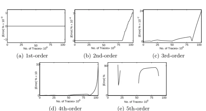
Fig. 1. Difference between the result of correlation estimations (raw-moment versus three-pass)

SincenL is limited, the above expression can be computed at the end when all traces are processed to estimate the correlation.

In the aforementioned approach the sumsSU M I(t)

l(a)

are grouped based on the

output of the leakage function, i.e.,l(a)_{, which is also key dependent. Hence, the}

traces have to be regrouped for each key candidate as well as for each selected leakage functioneL(.).

6

Evaluation

We evaluate the accuracy (convergence) of our presented approaches, and com-pare it to the corresponding results of the raw-moment and three-pass ap-proaches. To this end, we generate 100 million simulated leakages by∼N(100 +

HW(x),3), wherexis drawn uniformly from{0,1}4_{. Hence, the correlation}

be-tween the leakages and HW(x) is estimated. Following the concept of higher-order attacks, the leakages are also preprocessed (up to fifth higher-order) to allow an emulation of a higher-order univariate CPA. Note that the performance results are still valid in the multivariate case given additional leakage points with a sim-ilar leakage structure and the normalized product as combination function. This can be easily seen as both type of attacks require the estimation of centralized values up to a power of 2d (with an additional standardization for univariate higher-order attacks). The results based on our incremental approaches are ex-actly the same to the three-pass ones, i.e., with absolute 0 difference. As [3] only includes the formulas for first-order and second-order bivariate CPA, we further had to derive the necessary formulas for the univariate correlation up to the fifth order. The formulas can be found in Appendix E.

the same, but the differences start to be obvious at higher orders particularly for higher number of traces. It is noteworthy that in the cases where no difference is shown for the fifth-order correlation, one of the variances of the denominator in the raw-moment approach turned to a negative value which indicates the in-stability of such formulas. With respect to the execution time of each approach, although it depends on the optimization level of the underlying computer code, we report 43 s, 17.8 s, and 11.6 s for three-pass, our incremental, and raw-moment approach respectively to estimate all five correlations at the same time on 100 million leakage points. Obviously, the raw-moment approach is faster than the others due to its lower amount of computations compared to our incremental one.

Acknowledgment

The research in this work was supported in part by the DFG Research Training Group GRK 1817/1.

References

1. B. Bilgin, B. Gierlichs, S. Nikova, V. Nikov, and V. Rijmen. Higher-Order Thresh-old Implementations. InASIACRYPT 2014, volume 8874 ofLNCS, pages 326–343. Springer, 2014.

2. A. Bogdanov. Multiple-Differential Side-Channel Collision Attacks on AES. In

CHES 2008, volume 5154 ofLNCS, pages 30–44. Springer, 2008.

3. P. Bottinelli and J. W. Bos. Computational Aspects of Correlation Power Analysis. Cryptology ePrint Archive, Report 2015/260, 2015. http://eprint.iacr.org/. 4. E. Brier, C. Clavier, and F. Olivier. Correlation Power Analysis with a Leakage

Model. InCHES 2004, volume 3156 ofLNCS, pages 16–29. Springer, 2004. 5. S. Chari, C. S. Jutla, J. R. Rao, and P. Rohatgi. Towards Sound Approaches to

Counteract Power-Analysis Attacks. In CRYPTO 1999, volume 1666 ofLNCS, pages 398–412. Springer, 1999.

6. A. Duc, S. Dziembowski, and S. Faust. Unifying Leakage Models: From Probing Attacks to Noisy Leakage. InEUROCRYPT 2014, volume 8441 of LNCS, pages 423–440. Springer, 2014.

7. A. Duc, S. Faust, and F. Standaert. Making Masking Security Proofs Concrete -Or How to Evaluate the Security of Any Leaking Device. InEUROCRYPT 2015, volume 9056 ofLNCS, pages 401–429. Springer, 2015.

8. F. Durvaux, F.-X. Standaert, N. Veyrat-Charvillon, J.-B. Mairy, and Y. Deville. Efficient Selection of Time Samples for Higher-Order DPA with Projection Pur-suits. InCOSADE 2015, volume 9064 ofLNCS, pages 30–50. Springer, 2015. 9. G. Goodwill, B. Jun, J. Jaffe, and P. Rohatgi. A testing

method-ology for side channel resistance validation. In NIST non-invasive

attack testing workshop, 2011. http://csrc.nist.gov/news_events/

non-invasive-attack-testing-workshop/papers/08_Goodwill.pdf.

10. N. J. Higham. Accuracy and Stability of Numerical Algorithms (2. ed.). SIAM, 2002.

12. A. Moradi, O. Mischke, and T. Eisenbarth. Correlation-Enhanced Power Analysis Collision Attack. InCHES 2010, volume 6225 ofLNCS, pages 125–139. Springer, 2010.

13. A. Moradi, A. Poschmann, S. Ling, C. Paar, and H. Wang. Pushing the Limits: A Very Compact and a Threshold Implementation of AES. InEUROCRYPT 2011, volume 6632 ofLNCS, pages 69–88. Springer, 2011.

14. A. Moradi and F. Standaert. Moments-Correlating DPA. Cryptology ePrint Archive, Report 2014/409, 2014. http://eprint.iacr.org/.

15. P. P´ebay. Formulas for Robust, One-Pass Parallel Computation of Covariances and Arbitrary-Order Statistical Moments.Sandia Report SAND2008-6212, Sandia National Laboratories, 2008.

16. E. Prouff, M. Rivain, and R. Bevan. Statistical Analysis of Second Order Differ-ential Power Analysis. IEEE Trans. Computers, 58(6):799–811, 2009.

17. J. R. Rao, P. Rohatgi, H. Scherzer, and S. Tinguely. Partitioning Attacks: Or How to Rapidly Clone Some GSM Cards. InIEEE Symposium on Security and Privacy 2002, pages 31–41. IEEE Computer Society, 2002.

18. O. Reparaz, B. Gierlichs, and I. Verbauwhede. Selecting Time Samples for Mul-tivariate DPA Attacks. In CHES 2012, volume 7428 of LNCS, pages 155–174. Springer, 2012.

19. M. Rivain and E. Prouff. Provably Secure Higher-Order Masking of AES. InCHES 2010, volume 6225 ofLNCS, pages 413–427. Springer, 2010.

20. T. Schneider and A. Moradi. Leakage Assessment Methodology - a clear roadmap for side-channel evaluations. InCHES 2015, volume 9293 ofLNCS, pages 495–513. Springer, 2015.

21. F. Standaert, N. Veyrat-Charvillon, E. Oswald, B. Gierlichs, M. Medwed, M. Kasper, and S. Mangard. The World Is Not Enough: Another Look on Second-Order DPA. InASIACRYPT 2010, volume 6477 ofLNCS, pages 112–129. Springer, 2010.

22. Y. Zhou, Y. Yu, F. Standaert, and J. Quisquater. On the Need of Physical Security for Small Embedded Devices: A Case Study with COMP128-1 Implementations in SIM Cards. InFinancial Cryptography 2013, volume 7859 ofLNCS, pages 230–238. Springer, 2013.

A

Proof of Theorem 1

Proof. We start with the definition ofACSd,Qbased on Equation (11) and write

ACSd,Q=

X

(ti,li)∈Q

(ti−µt,Q)d(li−µl,Q)

= X

(ti,li)∈Q1

(ti−µt,Q)d(li−µl,Q) +

X

(ti,li)∈Q2

(ti−µt,Q)d(li−µl,Q).

(37)

M1,Q given in Equation (5) forµt,Qas well asµl,Qand write

X

(ti,li)∈Q1

(ti−µt,Q)d(li−µl,Q) =

X

(ti,li)∈Q1

ti−

n1µt,Q1+n2µt,Q2

n

d

li−

n1µl,Q1+n2µl,Q2

n

=

X

(ti,li)∈Q1

ti−µt,Q1−

n2

n ∆t

d

li−µl,Q1−

n2

n ∆l

(38)

Following [15] we write the first term of the product of Equation (38) as

ti−µt,Q1−

n2

n∆t

d

= (ti−µt,Q1) d

+

d−1

X

p=1

_d

p

(ti−µt,Q1) d−p

−n2 n∆t

p

+−n2 n∆t

d

(39)

By combining Equation (38) and Equation (39) we derive

X

(ti,li)∈Q1

(ti−µt,Q)

d

(li−µl,Q) =

ACSd,Q1+ d−1

X

p=1

_d

p

ACSd−p,Q1

−n2 n∆t

p

+CSd,Q1

−n2 n∆l

+

d−2

X

p=1

_d

p

CSd−p,Q1

−n2 n∆t

p

−n2 n ∆l

+n1

−n2 n∆t

d

−n2 n∆l

(40)

This can be simplified to

ACSd,Q1+CSd,Q1

−n2 n ∆l

+

d−1

X

p=1

d p

−n2 n∆t

p

ACSd−p,Q1+CSd−p,Q1

−n2 n∆l

+n1

−n2 n

d+1

(∆t) d

∆l (41)

It is noteworthy that CS1,Q1 is always zero and is ignored in the above

This procedure is repeated for the second sum of Equation (37), and we derive

X

(ti,li)∈Q2

(ti−µt,Q)d(li−µl,Q) =ACSd,Q2+CSd,Q2 n₁

n∆l

+

d−1

X

p=1

_d

p

n₁

n∆t

p

ACSd−p,Q2+CSd−p,Q2 n₁

n∆l

+n2

n₁

n

d+1

(∆t) d

∆l (42)

By combining Equation (41) and Equation (42) we obtain Equation (12). ut

B

Proof of Theorem 2

Proof. We start with the definition of the sum of the centralized product.

SCPd+1,Q,J0 =

X

V∈Q

Y

j∈J0

t(j)−µ(_Qj)

= X V∈Q1

Y

j∈J0

t(j)−µ(_Qj)+ X V∈Q2

Y

j∈J0

t(j)−µ(_Qj) (43)

Usingµ(_Qj)= n1µ

(j)

Q1+n2µ

(j)

Q2

n and∆

(j∈J0₎ =µ(_Qj)

2−µ

(j)

Q1, we rewrite the first sum

of Equation (43) as

X

V∈Q1 Y

j∈J0

t(j)−µ(_Qj)= X V∈Q1

Y

j∈J0

t(j)−n1µ

(j)

Q1+n2µ

(j)

Q2

n

!

= X V∈Q1

Y

j∈J0

t(j)−µ(_Qj)

1−

n2

n∆

(j)

=



 X

V∈Q1 Y

j∈J0

t(j)−µ(_Qj)

1





+



 d X

b=1

X

S∈Pb

X

V∈Q1 Y

s∈S

t(s)−µ(_Qs)

1

Y

j∈J0_\S n2∆(j)

−n





+



 X

V∈Q1 Y

j∈J0 n2∆(j)

−n



With Equation (18) and the fact that∀j ∈ J0_, X

V∈Q1

t(j)−µ(_Qj)= 0, we can simplify Equation (44) to

X

V∈Q1 Y

j∈J0

t(j)−µ(_Qj) = SCPd+1,Q1,J0+



 d X

b=2

X

S∈Pb

SCPb,Q1,S

Y

j∈J0_\S n2∆(j)

−n





+ (−n2)

d+1

n1

nd+1

Y

j∈J0

∆(j). (45)

By following the same procedure we can write the second sum of Equa-tion (43) as

X

V∈Q2 Y

j∈J0

t(j)−µ(_Qj) = SCPd+1,Q2,J0+



 d X

b=2

X

S∈Pb

SCPb,Q2,S

Y

j∈J0_\S n1∆(j)

n





+ n

d+1 1 n2

nd+1

Y

j∈J0

∆(j). (46)

The combination of (45) and (46) results in the iterative formula given in

C

Essential formulas for univariate CPA for up to

5th-order

C.1 Two-Pair Iterative

Below we consider ∆t =µt,Q2−µt,Q1 and ∆l =µl,Q2 −µl,Q1 with |Q1|=n1

and|Q2|=n2. The extended set is defined asQ=Q1∪ Q2with the cardinality

ofn. The computations related to the sample points should be repeated at each sample point separately.

Centralized Sums

CS2,L =CS2,L1+CS2,L2+n1n2 ∆_l

n

2

n1+n2

(see Equation (4)) (47)

CS2,Q=CS2,Q1+CS2,Q2+n1n2

∆

n

2

n1+n2

(48)

CS3,Q=CS3,Q1+CS3,Q2+

3∆ n

−n2CS2,Q1+n1CS2,Q2

+n1n2

∆

n

3

n12−n22

(49)

CS4,Q=CS4,Q1+CS4,Q2+

4∆ n

−n2CS3,Q1+n1CS3,Q2

+ 6∆ n

2

n22CS2,Q1+n1

2_CS 2,Q2

+n1n2

∆

n

4

n13+n23

(50)

CS5,Q=CS5,Q1+CS5,Q2+

5∆ n

−n2CS4,Q1+n1CS4,Q2

+ 10∆ n

2

n22CS3,Q1+n1

2_CS 3,Q2

+ 10∆ n

3

−n23CS2,Q1+n1

3_CS 2,Q2

+n1n2

∆

n

5

n14−n24

(51)

CS6,Q=CS6,Q1+CS6,Q2+

6∆ n

−n2CS5,Q1+n1CS5,Q2

+ 15∆ n

2

n22CS4,Q1+n1

2_CS 4,Q2

+ 20∆ n

3

−n23CS3,Q1+n1

3_CS 3,Q2

+ 15∆ n

4

n24CS2,Q1+n1

4_CS 2,Q2

+n1n2

∆

n

6

n15+n25

CS7,Q=CS7,Q1+CS7,Q2+

7∆ n

−n2CS6,Q1+n1CS6,Q2

+ 21∆ n

2

n22CS5,Q1+n1

2_CS 5,Q2

+ 35∆ n

3

−n23CS4,Q1+n1

3_CS 4,Q2

+ 35∆ n

4

n24CS3,Q1+n1

4_CS 3,Q2

+ 21∆ n

5

−n25CS2,Q1+n1

5_CS 2,Q2

+n1n2

∆

n

7

n16−n26

(53)

CS8,Q=CS8,Q1+CS8,Q2+

8∆ n

−n2CS7,Q1+n1CS7,Q2

+ 28∆ n

2

n22CS6,Q1+n1

2_CS 6,Q2

+ 56∆ n

3

−n23CS5,Q1+n1

3_CS 5,Q2

+ 70∆ n

4

n24CS4,Q1+n1

4_CS 4,Q2

+ 56∆ n

5

−n25CS3,Q1+n1

5_CS 3,Q2

+ 28∆ n

6

n26CS2,Q1+n1

6_CS 2,Q2

+n1n2

∆

n

8

n17+n27

(54)

CS9,Q=CS9,Q1+CS9,Q2+

9∆ n

−n2CS8,Q1+n1CS8,Q2

+ 36∆ n

2

n22CS7,Q1+n1

2_CS 7,Q2

+ 84∆ n

3

−n23CS6,Q1+n1

3_CS 6,Q2

+ 126∆ n

4

n24CS5,Q1+n1

4_CS 5,Q2

+ 126∆ n

5

−n25CS4,Q1+n1

5

CS4,Q2

+ 84∆ n

6

n26CS3,Q1+n1

6_CS 3,Q2

+ 36∆ n

7

−n27CS2,Q1+n1

7_CS 2,Q2

+n1n2

∆

n

9

n18−n28

CS10,Q=CS10,Q1+CS10,Q2+

10∆ n

−n2CS9,Q1+n1CS9,Q2

+ 45∆ n

2

n22CS8,Q1+n1

2_CS 8,Q2

+ 120∆ n

3

−n23CS7,Q1+n1

3_CS 7,Q2

+ 210∆ n

4

n24CS6,Q1+n1

4_CS 6,Q2

+ 252∆ n

5

−n25CS5,Q1+n1

5_CS 5,Q2

+ 210∆ n

6

n26CS4,Q1+n1

6_CS 4,Q2

+ 120∆ n

7

−n27CS3,Q1+n1

7_CS 3,Q2

+ 45∆ n

8

n28CS2,Q1+n1

8_CS 2,Q2

+n1n2

∆

n

10

n19+n29

(56)

Adjusted Centralized Sums

ACS1,Q= ACS1,Q1+ACS1,Q2+

n2(n1)2+n1(n2)2

n2 ∆t∆l (57)

ACS2,Q= ACS2,Q1+ACS2,Q2+

∆l

n (n1CS2,Q2−n2CS2,Q1)

+ 2

_∆

t

n

(n1ACS1,Q2−n2ACS1,Q1)

+n2(n1)

3

−n1(n2) 3

n3 (∆t) 2

∆l (58)

ACS3,Q= ACS3,Q1+ACS3,Q2+

∆l

n (n1CS3,Q2−n2CS3,Q1)

+3

_∆

t

n n1ACS2,Q2−n2ACS2,Q1+

∆l

n

(n1) 2

CS2,Q2+ (n2)

2

CS2,Q1

+3

_∆

t

n

2

(n1)2ACS1,Q2+ (n2)

2

ACS1,Q1

+n2(n1)

4

+n1(n2) 4

n4 (∆t) 3

ACS4,Q= ACS4,Q1+ACS4,Q2+

∆l

n (n1CS4,Q2−n2CS4,Q1)

+4

_∆

t

n n1ACS3,Q2−n2ACS3,Q1+

∆l

n

(n1)2CS3,Q2+ (n2)

2

CS3,Q1

+6

_∆

t

n

2

(n1)2ACS2,Q2+ (n2)

2

ACS2,Q1+

∆l

n

(n1)3CS2,Q2−(n2)

3

CS2,Q1

+4

_∆

t

n

3

(n1) 3

ACS1,Q2−(n2)

3

ACS1,Q1

+n2(n1)

5

−n1(n2) 5

n5 (∆t) 4

∆l (60)

ACS5,Q= ACS5,Q1+ACS5,Q2+

∆l

n (n1CS5,Q2−n2CS5,Q1)

+5

_∆

t

n n1ACS4,Q2−n2ACS4,Q1+

∆l

n

(n1)2CS4,Q2+ (n2)

2

CS4,Q1

+10

_∆

t

n

2

(n1) 2

ACS3,Q2+ (n2)

2

ACS3,Q1+

∆l

n

(n1) 3

CS3,Q2−(n2)

3

CS3,Q1

+10

∆t

n

3

(n1) 3

ACS2,Q2−(n2)

3

ACS2,Q1+

∆l

n

(n1) 4

CS2,Q2+ (n2)

4

CS2,Q1

+5

∆t

n

4

(n1) 4

ACS1,Q2+ (n2)

4

ACS1,Q1

+n2(n1)

6

+n1(n2)6

n6 (∆t) 5

∆l (61)

C.2 Incremental,n2= 1

Below we consider∆t=tn−µt,Q1 and∆l=ln−µl,Q1 with|Q1|=n−1. The

extended set is defined as Q=Q1∪

(tn, ln) with the cardinality ofn. The

computations related to the sample points should be repeated at each sample point independently.

Means and Centralized Sums

µt,Q=µt,Q1+

∆t

n µl,Q=µl,Q1+

∆l

CS2,L = CS2,L1+

(∆l)2(n−1)

n (see Equation (4)) (63)

CS2,Q= CS2,Q1+

(∆t)

2

(n−1)

n (64)

CS3,Q= CS3,Q1−

3∆t

n CS2,Q1+

(∆t)

3

(n−1)((n−1)2₋₁₎

n3 (65)

CS4,Q= CS4,Q1−

4∆t

n CS3,Q1+

6 (∆t)2

n2 CS2,Q1+

(∆t)4(n−1)((n−1)3+ 1)

n4

(66)

CS5,Q= CS5,Q1−

5∆t

n CS4,Q1+

10 (∆t)2

n2 CS3,Q1−

10 (∆t)3

n3 CS2,Q1

+(∆t)

5

(n−1)((n−1)4−1)

n5 (67)

CS6,Q= CS6,Q1−

6∆t

n CS5,Q1+

15 (∆t)2

n2 CS4,Q1−

20 (∆t)3

n3 CS3,Q1

+15 (∆t)

4

n4 CS2,Q1+

(∆t)

6

(n−1)((n−1)5+ 1)

n6 (68)

CS7,Q= CS7,Q1−

7∆t

n CS6,Q1+

21 (∆t)

2

n2 CS5,Q1−

35 (∆t)

3

n3 CS4,Q1

+35 (∆t)

4

n4 CS3,Q1−

21 (∆t)

5

n5 CS2,Q1+

(∆t)

7

(n−1)((n−1)6₋₁₎

n7

(69)

CS8,Q= CS8,Q1−

8∆t

n CS7,Q1+

28 (∆t)2

n2 CS6,Q1−

56 (∆t)3

n3 CS5,Q1

+70 (∆t)

4

n4 CS4,Q1−

56 (∆t)

5

n5 CS3,Q1+

28 (∆t)

6

n6 CS2,Q1

+(∆t)

8

(n−1)((n−1)7_{+ 1)}

n8 (70)

CS9,Q= CS9,Q1−

9∆t

n CS8,Q1+

36 (∆t)

2

n2 CS7,Q1−

84 (∆t)

3

n3 CS6,Q1

+126 (∆t)

4

n4 CS5,Q1−

126 (∆t)

5

n5 CS4,Q1+

84 (∆t)

6

n6 CS3,Q1

−36 (∆t)

7

n7 CS2,Q1+

(∆t)

9

(n−1)((n−1)8₋₁₎

CS10,Q= CS10,Q1−

10∆t

n CS9,Q1+

45 (∆t)

2

n2 CS8,Q1−

120 (∆t)

3

n3 CS7,Q1

+210 (∆t)

4

n4 CS6,Q1−

252 (∆t)

5

n5 CS5,Q1+

210 (∆t)

6

n6 CS4,Q1

−120 (∆t)

7

n7 CS3,Q1+

45 (∆t)

8

n8 CS2,Q1+

(∆t)

10

(n−1)((n−1)9_{+ 1)}

n10

(72)

Adjusted Centralized Sums

ACS1,Q= ACS1,Q1+

(n−1)2+n−1

n2 ∆t∆l (73)

ACS2,Q= ACS2,Q1−

∆l

n CS2,Q1−2

_∆

t

n

ACS1,Q1

+(n−1)

3

−n+ 1 n3 (∆t)

2

∆l (74)

ACS3,Q= ACS3,Q1−

∆l

n CS3,Q1−3

_∆

t

n ACS2,Q1−

∆l

n CS2,Q1

+ 3

_∆

t

n

2

ACS1,Q1+

(n−1)4+n−1 n4 (∆t)

3

∆l (75)

ACS4,Q= ACS4,Q1−

∆l

n CS4,Q1−4

_∆

t

n ACS3,Q1−

∆l

n CS3,Q1

+ 6

_∆

t

n

2

ACS2,Q1−

∆l

n CS2,Q1

−4

∆t

n

3

ACS1,Q1+

(n−1)5−n+ 1 n5 (∆t)

4

∆l (76)

ACS5,Q= ACS5,Q1−

∆l

n CS5,Q1−5

∆t

n ACS4,Q1−

∆l

n CS4,Q1

+ 10

_∆

t

n

2

ACS3,Q1−

∆l

nCS3,Q1

−10

_∆

t

n

3

ACS2,Q1−

∆l

nCS2,Q1

+ 4

_∆

t

n

4

ACS1,Q1+

(n−1)6+n−1 n6 (∆t)

5

At any time the correlation of a univariate CPA can be estimated as

(1st order) ρ=

1 nACS1

r

1 nCS2,Q

1 nCS2,L

(78)

(2nd order) ρ=

1 nACS2

v u u t

1

n CS4,Q−

(CS2,Q)

2

n

!

1 nCS2,L

(79)

(3rd order) ρ=

1 nACS3

v u u t

1

n CS6,Q−

(CS3,Q)2 n

!

1 nCS2,L

(80)

(4th order) ρ=

1 nACS4

v u u t

1

n CS8,Q−

(CS4,Q)

2

n

!

1 nCS2,L

(81)

(5th order) ρ=

1 nACS5

v u u t

1

n CS10,Q−

(CS5,Q)2 n

!

1 nCS2,L

(82)

D

Essential formulas for a bivariate second-order CPA

In the following we give the necessary formulas to the correlation for a bivariate second-order CPA for exemplary sample points J = {1,2}. Further, we con-sider J0 _{= {1,2,∗} with t}(∗)

i = li and t

(∗)

i = li. For the computation of the

denominator we also consider J00_={1,2,1,2}.

D.1 Two-Pair Iterative

We consider two setsQ1,Q2with|Q1|=n1,|Q2|=n2and∆(j∈J)=µ (j)

Q2−µ

(j)

Q1,

withµ(_Qj)

i as the mean of the setQiat sample pointj. The two sets make up the

Sum of Centered Products (Numerator)

SCP2,Q,{1,2}= SCP2,Q1,{1,2}+SCP2,Q2,{1,2}

+

(n1) 2

n2+n1(n2) 2

∆(1)_∆(2)

n2 (83)

SCP2,Q,{1,∗} = SCP2,Q1,{1,∗}+SCP2,Q2,{1,∗}

+

(n1) 2

n2+n1(n2) 2

∆(1)_∆(∗)

n2 (84)

SCP2,Q,{2,∗} = SCP2,Q1,{2,∗}+SCP2,Q2,{2,∗}

+

(n1)2n2+n1(n2)2

∆(2)_∆(∗)

n2 (85)

SCP3,Q,{1,2,∗} = SCP3,Q1,{1,2,∗}+SCP3,Q2,{1,2,∗}

+ n1SCP2,Q2,{1,2}−n2SCP2,Q1,{1,2}

∆

(∗)

n

+ n1SCP2,Q2,{1,∗}−n2SCP2,Q1,{1,∗}

∆

(2)

n

+ n1SCP2,Q2,{2,∗}−n2SCP2,Q1,{2,∗}

∆

(1)

n

+

(n1) 3

n2−n1(n2) 3

∆(1)∆(2)∆(∗)

n3 (86)

Sum of Centered Products (Denominator)

SCP2,Q,{1,1}= SCP2,Q1,{1,1}+SCP2,Q2,{1,1}

+

(n1)2n2+n1(n2)2

∆(1)_∆(1)

n2 (87)

SCP2,Q,{1,2}= SCP2,Q1,{1,2}+SCP2,Q2,{1,2}

+

(n1) 2

n2+n1(n2) 2

∆(1)_∆(2)

n2 (88)

SCP2,Q,{2,2}= SCP2,Q1,{2,2}+SCP2,Q2,{2,2}

+

(n1) 2

n2+n1(n2) 2

∆(2)∆(2)

SCP3,Q,{1,2,1}= SCP3,Q1,{1,2,1}+SCP3,Q2,{1,2,1}

+ n1SCP2,Q2,{1,2}−n2SCP2,Q1,{1,2}

2∆

(1)

n

+ n1SCP2,Q2,{1,1}−n2SCP2,Q1,{1,1}

∆

(2)

n

+

(n1) 3

n2−n1(n2) 3

∆(1)∆(2)∆(1)

n3 (90)

SCP3,Q,{1,2,2}= SCP3,Q1,{1,2,2}+SCP3,Q2,{1,2,2}

+ n1SCP2,Q2,{1,2}−n2SCP2,Q1,{1,2}

2∆

(2)

n

+ n1SCP2,Q2,{2,2}−n2SCP2,Q1,{2,2}

∆

(1)

n

+

(n1) 3

n2−n1(n2) 3

∆(1)∆(2)∆(2)

n3 (91)

SCP4,Q,{1,2,1,2}= SCP4,Q1,{1,2,1,2}+SCP4,Q2,{1,2,1,2}

+ n1SCP3,Q2,{1,2,1}−n2SCP3,Q1,{1,2,1}

2∆

(2)

n

+ n1SCP3,Q2,{1,2,2}−n2SCP3,Q1,{1,2,2}

2∆

(1)

n

+(n1)2SCP2,Q2,{1,2}+ (n2)2SCP2,Q1,{1,2}

2∆(1)∆(2)

n2

+(n1) 2

SCP2,Q2,{1,1}+ (n2)

2

SCP2,Q1,{1,1}

∆(2)∆(2)

n2

+(n1)2SCP2,Q2,{2,2}+ (n2)

2

SCP2,Q1,{2,2}

∆(1)∆(1)

n2

+

(n1) 4

n2+n1(n2) 4

∆(1)∆(2)∆(1)∆(2)

n4 (92)

D.2 Incremental,n2= 1

Below we consider ∆(j∈J) _=t(j)

n −µ(_Qj)

1 with |Q1|=n−1. The extended set is

defined asQ=Q1∪

(t(nj)|∀j∈ J) with the cardinality ofn.

Sum of Centered Products (Numerator)

SCP2,Q,{1,2}= SCP2,Q1,{1,2}+

(n−1)∆(1)_∆(2)

SCP2,Q,{1,∗}= SCP2,Q1,{1,∗}+

(n−1)∆(1)_∆(∗)

n (94)

SCP2,Q,{2,∗}= SCP2,Q1,{2,∗}+

(n−1)∆(2)∆(∗)

n (95)

SCP3,Q,{1,2,∗}= SCP3,Q1,{1,2,∗}−SCP2,Q1,{1,2}

∆(∗)

n

−SCP2,Q1,{1,∗} ∆(2)

n −SCP2,Q1,{2,∗} ∆(1)

n

+ n

2_{−3n+ 2}

∆(1)∆(2)∆(∗)

n2 (96)

Sum of Centered Products (Denominator)

SCP2,Q,{1,1}= SCP2,Q1,{1,1}+

(n−1)∆(1)∆(1)

n (97)

SCP2,Q,{1,2}= SCP2,Q1,{1,2}+

(n−1)∆(1)_∆(2)

n (98)

SCP2,Q,{2,2}= SCP2,Q1,{2,2}+

(n−1)∆(2)_∆(2)

n (99)

SCP3,Q,{1,2,1}= SCP3,Q1,{1,2,1}−2SCP2,Q1,{1,2} ∆(1)

n

−SCP2,Q1,{1,1}

∆(2)

n +

∆(1)_∆(2)_∆(1) _n2_{−3n+ 2}

n2 (100)

SCP3,Q,{1,2,2}= SCP3,Q1,{1,2,2}−2SCP2,Q1,{1,2} ∆(2)

n

−SCP2,Q1,{2,2}

∆(1)

n +

n2_{−3n+ 2}

∆(1)_∆(2)_∆(2)

n2 (101)

SCP4,Q,{1,2,1,2}= SCP4,Q1,{1,2,1,2}−2SCP3,Q1,{1,2,1}

∆(2)

n

−2SCP3,Q1,{1,2,2} ∆(1)

n +SCP2,Q1,{1,1}

∆(2)∆(2) n2

+ 4SCP2,Q1,{1,2}

∆(1)_∆(2)

n2 +SCP2,Q1,{2,2}

∆(1)_∆(1)

n2

+ n

3_−4n2_{+ 6n−3}

∆(1)_∆(2)_∆(1)_∆(2)

n3 (102)

At any time the correlation of a bivariate CPA can be estimated as

ρ=

1

nSCP3,Q,{1,2,∗}

r

1

nSCP4,Q,{1,2,1,2} 1 nCS2,L

, (103)

E

Correlation from the Raw Moments

As [3] only includes the formulas for first-order and second-order bivariate CPA, we first transform the bivariate formulas to the univariate second-order case and extend the approach to higher orders. Recall that the correlation for the bivariate second-order attack is computed in [3] as

ρ=_p nλ1−λ2s3 nλ3−λ22

√

ns9−s32

, (104)

where n denotes the number of traces andλ_{1,2,3} are derived from the sums s_{1,...,13}.

For the univariate second-order correlation, some of these sums are equiva-lent. Therefore, in this special case it is possible to reduce the number of sums required to be computed. For that, we first denote the d-th order sums as

S_d(t)=

n X

i=1

tdi, S

(l)

d =

n X

i=1

ldi, S

(t,l)

d =

n X

i=1

tdil (105)

withs3=S (l)

1 ands9=S (l)

2 . The remaining parameters are then derived as

λ1=S (t,l)

2 −2

S₁(t)S₁(t,l)

n +

S₁(t)S(₁t)S₁(l)

n2 , λ2=S (t)

2 −

S(₁t)S₁(t)

n , (106)

λ3=S (t) 4 −4

S₁(t)S₃(t) n + 6

S(₁t)S₁(t)S₂(t) n2 −3

S₁(t)S₁(t)S₁(t)S₁(t)

n3 . (107)

For the higher-order correlation the basic structure of Equation (104) stays the same, and only the formulas for λ{1,2,3} change. We provided all necessary for-mulas in the following subsections.

E.1 Third Order

λ1=S (t,l)

3 −3

S(₁t)S₂(t,l)

n + 3

S₁(t)

2

S₁(t,l)

n2 −

S₁(t)

3

S₁(l)

n3 , (108)

λ2=S (t) 3 −3

S₁(t)S₂(t) n + 2

S(₁t)

3

n2 , (109)

λ3=S (t) 6 −6

S₁(t)S₅(t) n + 15

S₁(t)

2

S₄(t)

n2 −20

S₁(t)

3

S₃(t)

n3

+ 15

S₁(t)

4

S₂(t)

n4 −5

S(₁t)

6

E.2 Fourth Order

λ1=S (t,l)

4 −4

S₁(t)S(₃t,l)

n + 6

S₁(t)

2

S(₂t,l)

n2 −4

S₁(t)

3

S(₁t,l)

n3 +

S₁(t)

4

S₁(l)

n4 ,

(111)

λ2=S (t) 4 −4

S(₁t)S₃(t) n + 6

S₁(t)

2

S₂(t)

n2 −3

S₁(t)

4

n3 , (112)

λ3=S (t) 8 −8

S(₁t)S₇(t) n + 28

S₁(t)

2

S₆(t)

n2 −56

S(₁t)

3

S₅(t)

n3

+ 70

S₁(t)

4

S₄(t)

n4 −56

S₁(t)

5

S₃(t)

n5 + 28

S₁(t)

6

S₂(t)

n6 −7

S₁(t)

8

n7 (113)

E.3 Fifth Order

λ1=S (t,l)

5 −5

S₁(t)S₄(t,l) n + 10

S(₁t)

2

S₃(t,l)

n2 −10

S₁(t)

3

S₂(t,l)

n3

+ 5

S₁(t)

4

S(₁t,l)

n4 −

S₁(t)

5

S₁(l)

n5 , (114)

λ2=S (t) 5 −5

S₁(t)S₄(t) n + 10

S₁(t)

2

S(₃t)

n2 −10

S₁(t)

3

S(₂t)

n3 + 4

S₁(t)

5

n4 , (115)

λ3=S (t) 10 −10

S₁(t)S₉(t) n + 45

S₁(t)

2

S₈(t)

n2 −120

S₁(t)

3

S(₇t)

n3 + 210

S₁(t)

4

S₆(t)

n4

−252

S₁(t)

5

S₅(t)

n5 + 210

S₁(t)

6

S₄(t)

n6 −120

S₁(t)

7

S(₃t)

n7 + 45

S₁(t)

8

S₂(t)

n8 −9

S(₁t)

10

n9