Getting even with CLE
GertAarts1,,KirillBoguslavski2,,ManuelScherzer3,,ErhardSeiler4,,DénesSexty5,†, andIon-OlimpiuStamatescu3,‡
1Physics Dept., Swansea Univ., UK, 2Physics Dept., Univ. of Jyväskylä, Finland,
3Institute for Theoretical Physics, Univ. Heidelberg, Germany, 4Max Plank Institute for Physics, München, Germany, 5Physics Dept., Wuppertal Univ, Germany,
Abstract.In the landscape of approaches toward the simulation of Lattice Models with complex action the Complex Langevin (CL) appears as a straightforward method with a simple, well defined setup. Its applicability, however, is controlled by certain specific conditions which are not always satisfied. We here discuss the procedures to meet these conditions and the estimation of systematic errors and present some actual achievements.
1 Introduction
For a model defined by a path integral with a complex action S, CL is a stochastic process proceeding on the complexification of the original manifold, e.g.,Rn−→CnorS U(n)−→S L(n,C). It involves a drift term K=−∇S and a suitably normalized random noiseη[1], cf also [2]. E.g., for one variable
x→z=x+iy the CL amounts to two real Langevin processes in the process time t δx(t) = Kx(z)δt+ηx(t), Kx=ReK(z), ηx=0, η2x=2NRδt
δy(t) = Ky(z)δt+ηy(t), Ky=ImK(z), ηy=0, η2y=2NIδt, NR−NI =1.
The process realises a real probability distribution P(x, y;t) accompanying the complex distribution ρ(x,t) (with asymptotic limit ρ(x)=exp(−S(x))). They evolve according to real (complex) FPE’s:
∂tP(x, y,t)=LTP(x, y,t), L=(NR∂x+Kx(z))∂x+(NI∂y+Ky(z)∂y ∂tρ(x,t)=LT0ρ(x,t), L0=(∂x+K(x))∂x.
Notice that an associated Random Walk process can also be defined: δx(t)= 0 with pbb. 1−q, or ±ωx with pbb. 12q (1±tanh(12ωxKx/
NR)), ωx= 2δt/q, δy(t)= 0 with pbb. 1−q, or ±ωy with pbb. 12q (1±tanh(12ωyKy/NI)), ωy= 2δt/q. The parametersq,NR, NIcan be chosen adequately; typically one takesNR =1,NI =0 andq1.
Acknowledges financial support from STFC, the Royal Society and the Wolfson Foundation.
Acknowledges finacial support from the European Research Council under grant No. ERC-2015-COG-681707. Acknowledges financial support from DFG under under grant STA 283/16-2.
Acknowledges financial support from DFG under under grant STA 283/16-2.
†Acknowledges financial support from DFG Heisenberg fellowship under grant SE 2466/1-1.
2 Conditions for convergence
For analytic observablesO(z) one can formally prove [3], [4]
O(z)P(x, y;t)dxdy=
O(x)ρ(x;t)dx. (1)
The proof of convergence relies on the holomorphy of the action and thus of the drift K, and on a well behaved distributionPat large values of the variables. Non-holomorphic behaviour is typically associated with zeroes of the measureρleading to a meromorphic drift K. Holomorphy can be regained by cutting small regions around the poles. The problem reduces therefore to the control of boundary terms both at∞and on the small contours around the poles. Their vanishing would ensure
LTP(x, y;t−τ)O(x+iy;τ)dxdy− P(x, y;t−τ)L O(x+iy;τ)dxdy=0; (2)
for anyτusing integration by parts and thus Eq. (1) [5], [8], cf. also [2].
In practice these conditions require quantitative estimations of the behaviour ofP(x, y) at largeyor near the poles of the driftK(x, y) [5], which in realistic cases need on-line or a posteriori estimations. This implies approximations in interpreting the data and induces systematic errors. This is familiar from other simulations algorithms: reweighting, R-algorithm, cooling or Wilson flow, etc.
The CL process can be redefined in many ways while still leading to the same expectation values, see discussion in [6] and further work cited there. In particular for gauge theories one efficient method is to keep the process near theS U(3) manifold by gauge transformations (gauge cooling[7]) minimis-ing some measure of non-unitarity, such as a “unitarity norm” NU=tr(U U†)−3,U∈S L(3,C). One can envisage various ways of defining such cooling procedures by minimising also other quantities, see e.g. [8]. Other transformations of the process have been investigated [10].
3 Lessons from simple models
We shall consider here an effective model defined as the nontrivial link U ∈S L(3,C) of a temporal gauge Polyakov loop in the field of its neighbours. Further simple models are discussed in [2], [5]. After transforming to the Cartan basis the action reads:
−S =β 3
i=1
eαieiwi+e−αie−iwi+lnD+lnH,
3
i=1
wi=0,U=diag{eiwi}, O
n=trUn (3)
withHtheS L(3,C) Haar measure.α∈Csimulate the staples. The fermionic determinant is:
D=DD˜2, D=1+C3 1+a P+bP˜, D˜ =1+C˜3 1+a˜P˜+b P˜ , (4) C=(2κeµ)Nτ, a=3C/(1+C3), b=C a, ˜C=(2κe−µ)Nτ,˜a=3 ˜C/(1+ ˜C3), ˜b= ˜C ˜a
P= 13trU, P˜ =13trU−1 (5)
At largeµwe can set ˜D 1. The parametersa,bhave maxima of height 22/3 atC = 2∓1/3. We expect effects from the zeroes of the determinant whena,b>1. We present results in terms ofµfor a targeted 4-dim. lattice model withNτ=8 andκ =0.12. The only relevant parameter isCand the
interesting region is aroundC=1 which meansµ1.425. The “bad” intervala,b>1 corresponds to 1.29< µ <1.56. Largerκshifts thea,bpeaks to smallerµ, largerNτmakes them sharper.
2 Conditions for convergence
For analytic observablesO(z) one can formally prove [3], [4]
O(z)P(x, y;t)dxdy=
O(x)ρ(x;t)dx. (1)
The proof of convergence relies on the holomorphy of the action and thus of the drift K, and on a well behaved distributionPat large values of the variables. Non-holomorphic behaviour is typically associated with zeroes of the measureρleading to a meromorphic drift K. Holomorphy can be regained by cutting small regions around the poles. The problem reduces therefore to the control of boundary terms both at∞and on the small contours around the poles. Their vanishing would ensure
LTP(x, y;t−τ)O(x+iy;τ)dxdy− P(x, y;t−τ)L O(x+iy;τ)dxdy=0; (2)
for anyτusing integration by parts and thus Eq. (1) [5], [8], cf. also [2].
In practice these conditions require quantitative estimations of the behaviour ofP(x, y) at largeyor near the poles of the driftK(x, y) [5], which in realistic cases need on-line or a posteriori estimations. This implies approximations in interpreting the data and induces systematic errors. This is familiar from other simulations algorithms: reweighting, R-algorithm, cooling or Wilson flow, etc.
The CL process can be redefined in many ways while still leading to the same expectation values, see discussion in [6] and further work cited there. In particular for gauge theories one efficient method is to keep the process near theS U(3) manifold by gauge transformations (gauge cooling[7]) minimis-ing some measure of non-unitarity, such as a “unitarity norm” NU=tr(U U†)−3,U∈S L(3,C). One can envisage various ways of defining such cooling procedures by minimising also other quantities, see e.g. [8]. Other transformations of the process have been investigated [10].
3 Lessons from simple models
We shall consider here an effective model defined as the nontrivial link U∈S L(3,C) of a temporal gauge Polyakov loop in the field of its neighbours. Further simple models are discussed in [2], [5]. After transforming to the Cartan basis the action reads:
−S =β 3
i=1
eαieiwi+e−αie−iwi+lnD+lnH,
3
i=1
wi=0, U=diag{eiwi}, O
n=trUn (3)
withHtheS L(3,C) Haar measure.α∈Csimulate the staples. The fermionic determinant is:
D=DD˜2, D=1+C3 1+a P+bP˜, D˜ =1+C˜3 1+a˜P˜+b P˜ , (4) C=(2κeµ)Nτ, a=3C/(1+C3), b=C a, ˜C=(2κe−µ)Nτ,˜a=3 ˜C/(1+ ˜C3), ˜b= ˜C ˜a
P= 13trU, P˜ =13trU−1 (5)
At largeµwe can set ˜D 1. The parametersa,b have maxima of height 22/3 atC = 2∓1/3. We expect effects from the zeroes of the determinant whena,b>1. We present results in terms ofµfor a targeted 4-dim. lattice model withNτ=8 andκ=0.12. The only relevant parameter isCand the
interesting region is aroundC=1 which meansµ1.425. The “bad” intervala,b >1 corresponds to 1.29< µ <1.56. Largerκshifts thea,bpeaks to smallerµ, largerNτmakes them sharper.
To illustrate the effect of the neighbours we consider two cases (“ordered” and “disordered”): 0: {α}=0, 1: {α}={0.2+1.5 i; −0.2+3.1 i; 0.2−0.7 i}.
-0.04 -0.02 0 0.02 0.04
-1 0 1 2 3 4 5 6 7 8
zdet, mu=1.425, t>1000, ReD>0: red ReD<0: blue
-1 0 1 2 3 4 5 6 7 8
0 5000 10000 15000 20000
-0.2 -0.15 -0.1 -0.05 0 0.05 0.1 0.15 0.2
-1 0 1 2 3 4 5 6 7 8
zdet, mu=1.425, dmin>10-6: red dmin<10-6: blue
-1 0 1 2 3 4 5 6 7 8
0 5000 10000 15000 20000
0 0.0005 0.001 0.0015 0.002 0.0025 0.003
-2 0 2 4 6 8 10
Nt=8, NU vs ReD ReD distribution
-2 -1 0 1 2 3
-2 0 2 4 6 8 10
Nt=8, O2 vs ReD alsim=-0.5431 w+sim=-0.6486 exact=-0.6487 w+ ex=-0.6487 w- ex=-0.2044
Figure 1. One link effective model, Nτ =8, κ =0.12,µ = 1.425 (“bad” point). Top: scatter plot ofDand trajectory histories for the ordered case.Middle: same for the disordered case. Bottom: histogram of ReDand correlation ofNUand ReD(left plot) and of the observableO2and ReD(right plot). See also the text.
The scatter plots forDshow a peculiar structure in the “bad" interval (absent outside of it). Here the process also samples two exceptional regions (blue in the upper plots of Fig. 1) characterized by ReD<0. They contribute wrong values for the observables. They are connected by a bottleneck at D=0 to the “red" region, therefore ReD<0 contributions come from trajectories which went near D=0. Trajectories starting in “blue" typically switch to “red" and only rarely visit “blue” again.
-0.5 0 0.5 1
1.41 1.415 1.42 1.425 1.43 1.435 1.44 1.445 1.45
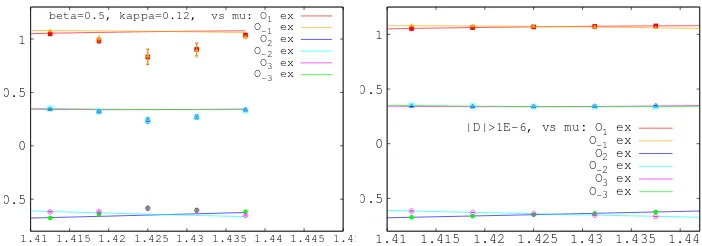
beta=0.5, kappa=0.12, vs mu: O1 ex
O-1 ex O2 ex O-2 ex O3 ex O-3 ex
-0.5 0 0.5 1
1.41 1.415 1.42 1.425 1.43 1.435 1.44 |D|>1E-6, vs mu: O1 ex
O-1 ex O2 ex O-2 ex
O
3 ex
O-3 ex
Figure 2. One link model,Nτ=8, κNτ=0.12: Observables vsµfrom all regions and from the “red” region.
4 From simple models to QCD
4.1 The Polyakov chain model
A Polyakov chain ofNτlinks allows to test procedures involving full gauge field integration of many
links [7]. Since it can be reduced by gauge transformations to the one link model of Sec. 3one can compare with exact results. On the other hand, the direct integration in the full group space over the
Nτlinks allows to see the effects of accumulation of round-offerrors, cooling, etc. This model is a
step toward HD-QCD which is no longer exactly solvable.
We shall consider two versions, referred to as model 1 and model 2 below:
1 : −S1 = β(P+P˜)+2nfln(1+aP+bP˜), 2 : −S2=(β+2nfa)P+(β+2nfb) ˜P, (6)
P = tr
Nτ
t=1
Ut, P˜=tr
Nτ
t=1 Ut
−1
(7)
witha,bof Sec.3andnf the number of flavours. CL proceeds in the group algebra:
U
t =exp
−
a
iλa(DatS[U]+ √ηat)
Ut (8)
withDa: covariant derivative. Model 1 is the direct extension of that in Sec. 3, model 2 is the un-resummed version of model 1 [11] and has no zeroes. We test two “cooling" methods to control the drift in the noncompact direction by minimising:
I : NU =
t
(tr(UtU†t)−3), II : NI =
t
a
ImDa
tS[U]2 (9)
This proceeds by non-compact gauge transformations using the covariant gradients of the norms. In Table1we show typical results forβ=0.5,Nτ =8, κ=0.12, µ=1.4, =10−5(non-adaptive). We
cool after each updating step: one sweep Cooling I (1 0), one sweep Cooling II (0 1), or both (1 1). The best results are obtained with more cooling sweeps. Remarks:
- It appears important to start in or near theS U(3) manifold and to cool during thermalisation; - The value ofNUcan vary (if it stays below 0.1), especially with (1,1) cooling;
-0.5 0 0.5 1
1.41 1.415 1.42 1.425 1.43 1.435 1.44 1.445 1.45
beta=0.5, kappa=0.12, vs mu: O1 ex
O-1 ex O2 ex O-2 ex O3 ex O-3 ex
-0.5 0 0.5 1
1.41 1.415 1.42 1.425 1.43 1.435 1.44 |D|>1E-6, vs mu: O1 ex
O-1 ex O2 ex O-2 ex
O
3 ex
O-3 ex
Figure 2. One link model,Nτ=8, κNτ=0.12: Observables vsµfrom all regions and from the “red” region.
4 From simple models to QCD
4.1 The Polyakov chain model
A Polyakov chain ofNτlinks allows to test procedures involving full gauge field integration of many
links [7]. Since it can be reduced by gauge transformations to the one link model of Sec. 3one can compare with exact results. On the other hand, the direct integration in the full group space over the
Nτlinks allows to see the effects of accumulation of round-offerrors, cooling, etc. This model is a
step toward HD-QCD which is no longer exactly solvable.
We shall consider two versions, referred to as model 1 and model 2 below:
1 : −S1 = β(P+P˜)+2nfln(1+aP+bP˜), 2 : −S2=(β+2nfa)P+(β+2nfb) ˜P, (6)
P = tr
Nτ
t=1
Ut, P˜=tr
Nτ
t=1 Ut
−1
(7)
witha,bof Sec. 3andnf the number of flavours. CL proceeds in the group algebra:
U
t =exp
−
a
iλa(DatS[U]+ √ηat)
Ut (8)
withDa: covariant derivative. Model 1 is the direct extension of that in Sec. 3, model 2 is the un-resummed version of model 1 [11] and has no zeroes. We test two “cooling" methods to control the drift in the noncompact direction by minimising:
I : NU=
t
(tr(UtUt†)−3), II : NI =
t
a
ImDa
tS[U]2 (9)
This proceeds by non-compact gauge transformations using the covariant gradients of the norms. In Table1we show typical results forβ=0.5,Nτ =8, κ =0.12, µ=1.4, =10−5(non-adaptive). We
cool after each updating step: one sweep Cooling I (1 0), one sweep Cooling II (0 1), or both (1 1). The best results are obtained with more cooling sweeps. Remarks:
- It appears important to start in or near theS U(3) manifold and to cool during thermalisation; - The value ofNUcan vary (if it stays below 0.1), especially with (1,1) cooling;
- For model 1 cooling also seems to improve concerning the effects of the non-holomorphy.
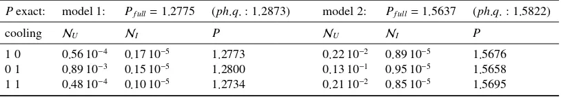
Table 1.Comparing cooling types for the Polyakov chain model. The statistical errors areO(10−3).
Pexact: model 1: Pf ull=1.2775 (ph.q.: 1.2873) model 2: Pf ull=1.5637 (ph.q.: 1.5822)
cooling NU NI P NU NI P
1 0 0.56 10−4 0.17 10−5 1.2773 0.22 10−2 0.89 10−5 1.5676
0 1 0.89 10−3 0.15 10−5 1.2800 0.13 10−1 0.95 10−5 1.5658
1 1 0.48 10−4 0.10 10−5 1.2734 0.21 10−2 0.85 10−5 1.5695
4.2 HD-QCD
HD-QCD arises in the limitκ → 0, µ → ∞where the determinant of QCD becomes a product of factors Eq. (4) over all Polyakov loops [12]. Calculations have explored among other things the phase diagram of the model , see e.g. [13] (reweighting), [14] (CL).
As before, the correctness of the results depends on the weight of the ReD<0 regions, which was there typicallyO(10−2−10−4) and we found a corresponding systematic error of the same magnitude. Now this weight and the associated systematic error are difficult to estimate, due to the superposition of single regions in the product of factors which define the determinant. We therefore need direct simulations and tests. Comparing CLE and reweighting in the region where the latter is reliable (µ <1 with phase rewighting) [13] we have observed generally good agreement but increasing deviations for β≤5.7 [7]. Lower temperatures require therefore largeNτ which would permit to work at largeβ.
This appears to be a question of computer power but further tests may be necessary.
4.3 Full QCD in theκexpansion
Splitting the fermionic determinant into temporal and spatial contributions we evaluate the first factor analytically (HD-QCD) and use a hopping expansion for the spatial part [15], [16]. This was shown to converge towards full QCD at sensible parameter choices already around order ten [15].
As we have learned from HD-QCD we needβ > 5.7 for the gauge cooling to be effective. Here we stay withβ=6. We present for illustration preliminaryO(κ10) results on lattices of 103×Nτ at β=6, κ =0.12, aimed at the phase diagram of QCD. For an investigative study trying to reach low temperatures we use largeNτbut are aware of the finite size effects induced by the wrong aspect ratio.
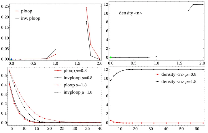
In the upper two plots of Fig. 3we fix a rather low temperatureNτ =16 and varyµ. It appears
that we can explore both the confining and the deconfining phase. Atµ=0 the gauge cooling ensures that the results agree with those obtained by reunitarisation, which is equivalent to a real Langevin simulation (blue and green dots atµ = 0 on the plots). Notice that the agreement may be lost by choosing an inadequateβ <6 where cooling becomes ineffective [17], [18].
In the lower two plots of Fig. 3we vary the temperatureT =1/Nτby increasingNτat fixedµ.
Starting at high temperature in the deconfining phase forµ≤1.1 we see the signal of the transition to the confining phase atT ∼0.1 (Nτ 10), especially perspicuous in the Polyakov loops. Atµ≥1.8
we see fully saturated density at low temperature and slightly decreasing at higherT.
In the region 0 ≤ µ ≤ 1.1 cooling is effective and we observe the silver blaze phenomenon expected in the confining region already atNτ = 16. Likewise the region ofµ ≥ 1.8 is accessible
●
● ● ● ● ●
●
■
■
■
■ ■
■
■
●
●
●
■
■
■
● ● ■ ■
● ploop
■ inv. ploop
0.0 0.5 1.0 1.5 2.0
0.00 0.05 0.10 0.15 0.20 0.25
● ● ● ● ● ●
●
●
● ●
● ●
●
density<n>
0.0 0.5 1.0 1.5 2.0
0 2 4 6 8 10 12
●
●
● ●
●
● ● ● ● ● ●
■
■
■
■ ■
■ ■ ■ ■ ■ ■
◆
◆
◆
◆ ◆
◆ ◆
◆
◆ ◆ ◆
▲
▲
▲
▲
▲
▲
▲ ▲ ▲ ▲ ▲
● ploopμ=0.8
■ invploopμ=0.8
◆ ploopμ=1.8
▲ invploopμ=1.8
5 10 15 20 25 30 35 40
0.0 0.1 0.2 0.3 0.4 0.5
●
●●●●●●● ● ● ● ● ● ●
■ ■
■■
■■■■ ■ ■ ■ ■ ■ ■
● density<n>μ=0.8
■ density<n>μ=1.8
10 20 30 40 50 60
0 2 4 6 8 10 12
Figure 3.QCD inκexpansion,β=6, κ=0.12.Top:µ-dependence of the Polyakov loop (left) and of the density (right) at fixedNτ=16.Bottom:Nτ-dependence of the Polyakov loop (left) and of the density at fixedµ(right).
5 Further prospects:
S U
(2)
real time simulations
Revisiting direct simulations of the Minkowski action inS U(2) [21], [22], the use of gauge cooling [7] and dynamical stabilisation [10] show promising improvements. Various integration contours are possible [22], [23], we found as optimal an isosceles triangle with base of extension τ along the imaginary axis and of extensiont0in the real time direction, discretised inNtpoints.
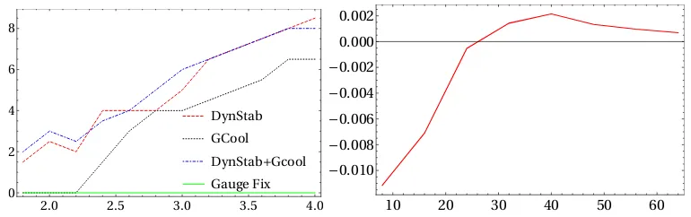
The left plot of Fig. 4depicts the maximum possible real time extentt0of the contour for fixed τ=16 andNt=16. Here gauge fixing fails but gauge cooling and dynamical stabilisation allow for a non-zero real-time extent in an interestingβ-region. Note that for smallNtthere can be deviations in the expectation value of the spatial plaquette between the euclidean and the real-time contour. This difference however becomes smaller as one increasesNt. The right plot depicts the difference as a function ofNt at fixedt0. . The discretisation oft0,Nt, is relevant. Largerβallow larger real time extents. The maximum extent oft0strongly depends onτ. For smallerτlarger ratiost0/τare possible.
6 Conclusions
● ● ● ● ● ● ● ■ ■ ■ ■ ■ ■ ■ ● ● ● ■ ■ ■ ● ●■■ ● ploop
■ inv. ploop
0.0 0.5 1.0 1.5 2.0
0.00 0.05 0.10 0.15 0.20 0.25 ● ● ● ● ● ● ● ● ● ● ● ● ● density<n>
0.0 0.5 1.0 1.5 2.0
0 2 4 6 8 10 12 ● ● ● ● ● ● ● ● ● ● ● ■ ■ ■ ■ ■ ■ ■ ■ ■ ■ ■ ◆ ◆ ◆ ◆ ◆ ◆ ◆ ◆ ◆ ◆ ◆ ▲ ▲ ▲ ▲ ▲ ▲ ▲ ▲ ▲ ▲ ▲
● ploopμ=0.8
■ invploopμ=0.8
◆ ploopμ=1.8
▲ invploopμ=1.8
5 10 15 20 25 30 35 40
0.0 0.1 0.2 0.3 0.4 0.5 ● ●●●●●●● ● ● ● ● ● ● ■ ■ ■■ ■■■■ ■ ■ ■ ■ ■ ■
● density<n>μ=0.8
■ density<n>μ=1.8
10 20 30 40 50 60
0 2 4 6 8 10 12
Figure 3.QCD inκexpansion,β=6, κ=0.12.Top:µ-dependence of the Polyakov loop (left) and of the density (right) at fixedNτ=16.Bottom:Nτ-dependence of the Polyakov loop (left) and of the density at fixedµ(right).
5 Further prospects:
S U
(2)
real time simulations
Revisiting direct simulations of the Minkowski action inS U(2) [21], [22], the use of gauge cooling [7] and dynamical stabilisation [10] show promising improvements. Various integration contours are possible [22], [23], we found as optimal an isosceles triangle with base of extension τ along the imaginary axis and of extensiont0in the real time direction, discretised inNtpoints.
The left plot of Fig. 4depicts the maximum possible real time extentt0of the contour for fixed τ=16 andNt=16. Here gauge fixing fails but gauge cooling and dynamical stabilisation allow for a non-zero real-time extent in an interestingβ-region. Note that for smallNtthere can be deviations in the expectation value of the spatial plaquette between the euclidean and the real-time contour. This difference however becomes smaller as one increases Nt. The right plot depicts the difference as a function ofNtat fixedt0. . The discretisation oft0,Nt, is relevant. Largerβallow larger real time extents. The maximum extent oft0strongly depends onτ. For smallerτlarger ratiost0/τare possible.
6 Conclusions
Gauge cooling[7] (and its further developments) appear essential for controlling the behaviour of the CL distributions both in the far non-compact direction and near the poles [5], see also [1]. The efficiency of the CL method for lattice gauge theories therefore strongly depends on the effectiveness of cooling. The latter can be judged from the unitarity normNUwhich is expected to stabilise at some value fixed by the dynamics. In the simulation numerical errors may eventually lead to a divergence ofNU, but as long asNUstays bounded we can sample reliable results.
DynStab
GCool
DynStab+Gcool
Gauge Fix
2.0 2.5 3.0 3.5 4.0
0 2 4 6 8
10 20 30 40 50 60
-0.010 -0.008 -0.006 -0.004 -0.002 0.000 0.002
Figure 4. S U(2) real time evolution. LeftMaximal possible real time extentt0vs. βforNs =8,Nt =16 and
inverse temperatureτ=16.Right: Difference of the spatial plaquette between the euclidean and the symmetric triangle contour with real time extentt0=3 as a function ofNtatβ=3,Ns=16.
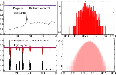
The evolution of theNUunder cooling permits to judge the efficiency of the latter and therefore the reliability of the results - see Fig. 5. Isolated peaks do not spoil the simulation as long as there are sufficiently long intervals of small unitarity norm. Removing the occasional peaks and selecting the intervals of smallNU leads then to well behaved distributions and correct convergence of the simulation (remember that cooling is a gauge transformation). For tests of other cooling procedures see, e.g. [8], [9], [10].
For QCD lattice calculations atµ >0 our results in a 10-th orderκexpansion show that simulations in the confinement and deconfining phases are possible forβlarge enough. Work in progress concerns resolving the phase transition region. Low temperatures require large lattices in order to ensure a good aspect ratio. A lesson from the study of simple models is to check the appearence of domains with ReD<0, drop their contributions and estimate a possible systematic error. As shown in [5] the signal is already visible in the observables and can thus be easily monitored.
For SU(2) real time evolution cooling and dynamical stabilisation are shown to improve the sim-ulations also for smallerβ, future work is however still necessary to achieve realistic scenarios.
References
[1] G. Aarts, L. Bongiovanni, E. Seiler, D. Sexty, I.-O. Stamatescu, Eur. Phys. J. A 49 (2013) 89 [arXiv:1303.6425 [hep-lat]]
[2] E. Seiler, these proceedings.
[3] G. Aarts, E. Seiler and I. O. Stamatescu, Phys. Rev. D81(2010) 054508 [arXiv:0912.3360 [hep-lat]]. [4] G. Aarts, F. A. James, E. Seiler and I. O. Stamatescu, Eur. Phys. J. C71(2011) 1756 [arXiv:1101.3270
[hep-lat]].
[5] G. Aarts, E. Seiler, D. Sexty and I.-O. Stamatescu, JHEP1705(2017) 044 [arXiv:1701.02322 [hep-lat]]. [6] G. Aarts, F. A. James, J. M. Pawlowski, E. Seiler, D. Sexty and I.-O. Stamatescu, JHEP03(2013) 073,
[arxiv: 1212.5231 [hep-lat]].
[7] E. Seiler, D. Sexty and I.-O. Stamatescu, Phys. Lett. B723(2013) 213, [arXiv:1211.3709 [hep-lat]]. [8] K. Nagata, J. Nishimura and S. Shimasaki, Phys. Rev. D94(2016) no.11, 114515 [arXiv:1606.07627
[hep-lat]].
[9] K. Nagata, H. Matsufuru, J. Nishimura and S. Shimasaki, PoS LATTICE 2016 (2016) 067 [arXiv:1611.08077 [hep-lat]].
Plaquette Unitarity Norm x 50
<plaquette>
0 10 20 30 40
0.0 0.1 0.2 0.3 0.4 0.5 0.6
0.588 0.590 0.592 0.594 0.596 0.598
0.5 1 5 10
Plaquette Unitarity Norm/2
Exact plaquette
0 200 400 600 800
0.0 0.2 0.4 0.6 0.8 1.0 1.2
0.88 0.89 0.90 0.91 0.92 0.93
0.5 1 5 10 50 100
Figure 5. Cooling effectiveness. Top: QCD inκexpansion,β= 6, κ =0.12,Nτ =16, Langevin evolution with cooling (12 sweeps per dynamical sweep) ofNU and the plaquette (left) and histogram of the latter using
the regions of boundedNU (right). Bottom: S U(2) real time on the isoscel triangle,Ns =4,Nt =8,β =16,
Langevin evolution with cooling (2 sweeps) of the unitarity norm and the spatial plaquette (left) and histogram of the plaquette usingNU<0.07 (right). Before discarding the peaks inNUthe histograms had pronounced skirts.
[11] I.-O. Stamatescu and E. Seiler, PoS LATTICE2016, 357 (2016) [arXiv:1611.00620 [hep-lat]].
[12] I. Bender, T. Hashimoto, F. Karsch, V. Linke, A. Nakamura, M. Plewnia, I.-O. Stamatescu and W. Wetzel, Nucl. Phys. Proc. Suppl.26, 323 (1992).
[13] R. De Pietri, A. Feo, E. Seiler and I.-O. Stamatescu, Phys. Rev. D76(2007) 114501 [arXiv:0705.3420 [hep-lat]].
[14] G. Aarts, F. Attanasio, B. Jäger and D. Sexty, JHEP1609(2016) 087 [arXiv:1606.05561 [hep-lat]]. [15] G. Aarts, E. Seiler, D. Sexty and I.-O. Stamatescu, Phys. Rev. D90, 114505 (2014), [arXiv:1408.3770
[hep-lat]].
[16] M. Fromm, J. Langelage, S. Lottini and O. Philipsen, JHEP1201(2012) 042 [arXiv:1111.4953 [hep-lat]]. [17] J. Bloch and O. Schenk, [arXiv:1707.08874 [hep-lat]].
[18] D. K. Sinclair and J. B. Kogut, PoS LATTICE2016, 026 (2016), [arXiv:1611.02312 [hep-lat]]. [19] S. Schmalzbauer and J. Bloch, PoS LATTICE2016(2016) 362 [arXiv:1611.00702 [hep-lat]]. [20] D. Sexty, Phys. Lett. B729(2014) 108 [arXiv:1307.7748 [hep-lat]].
[21] J. Berges and D. Sexty, Nucl. Phys. B799(2008) 306 [arXiv:0708.0779 [hep-lat]].
[22] J. Berges, S. Borsanyi, D. Sexty and I.-O. Stamatescu, Phys. Rev. D75(2007) 045007 [hep-lat/0609058]. [23] A. Alexandru, G. Basar, P. F. Bedaque, S. Vartak and N. C. Warrington, Phys. Rev. Lett.117(2016) 081602