Article
Skin Doctor: Machine Learning Models for Skin
Sensitization Prediction that Provide Estimates and
Indicators of Prediction Reliability
Anke Wilm 1,2, Conrad Stork 1, Christoph Bauer 3,4, Andreas Schepky 5, Jochen Kühnl 5 and Johannes Kirchmair 1,3,4*
1 Center for Bioinformatics, Universität Hamburg, Hamburg, Germany 2 HITeC e.V, Hamburg, Germany
3 Department of Chemistry, University of Bergen, Bergen, Norway
4 Computational Biology Unit (CBU), University of Bergen, Bergen, Norway 5 Front End Innovation, Beiersdorf AG, Hamburg, Germany
* Correspondence: [email protected]; Tel.: +49-40-42838-7303.
Abstract: The ability to predict the skin sensitization potential of small organic molecules is of high importance to the development and safe application of cosmetics, drugs and pesticides. One of the most widely accepted methods for predicting this hazard is the rodent local lymph node assay (LLNA). The goal of this work was to develop in silico models for the prediction of the skin sensitization potential of small molecules that go beyond the state of the art, with larger LLNA data sets and, most importantly, a robust and intuitive definition of the applicability domain, paired with additional indicators of the reliability of predictions. We explored a large variety of molecular descriptors and fingerprints in combination with random forest and support vector machine classifiers. The most suitable models were tested on holdout data, on which they yielded competitive performance (Matthews correlation coefficients up to 0.52; accuracies up to 0.76; areas under the receiver operating characteristic curves up to 0.83). The most favorable models are available via a public web service at https://nerdd.zbh.uni-hamburg.de/skinDoctor/ that, in addition to predictions, provides assessments of the applicability domain and indicators of the reliability of the individual predictions.
Keywords: skin sensitization potential; prediction; in silico models; machine learning; local lymph node assay (LLNA); cosmetics; drugs; pesticides; chemical space; applicability domain
1. Introduction
Repeated exposure to reactive chemicals with skin-sensitizing properties can cause allergic contact dermatitis (ACD) [1], an adverse cutaneous condition with a prevalence of ~20% among the general population [2] and even higher prevalence among workers with chronic occupational exposure [3]. Understanding the skin sensitization potential of small organic molecules is therefore of essence to the development and safe application of chemicals, including cosmetics and drugs.
Historically, animal tests have effectively been the only method for determining the skin sensitization potential and potency of substances. The rodent local lymph node assay (LLNA) is currently considered to be the most advanced animal testing system [4]. In recent years, ethical considerations and regulatory requirements have led to an intensification of the search for alternatives to animal testing, in particular in the cosmetics industry [5]. New in vitro and in chemico methods have been developed and evaluated [6–9], and computational approaches are starting to be recognized as important alternatives to animal testing [8–11]. The non-redundant combinatorial use of said methods in defined approaches that assess several key events of the adverse outcome pathway (AOP) for skin sensitization shows promising predictive capacity [12] and is currently evaluated in risk assessment case studies.
The bottleneck in the development of in silico tools for the prediction of skin sensitization is not related to technology but to the scarcity of available high quality experimental data for model development. Three strategies have been pursued to address this problem. The first one is to increase the amount and coverage of data by employing data mining techniques to retrieve information from various types of assays and sources [13,14]. Though this has been discussed as a promising strategy to increase the applicability of models it has also prompted controversial discussions regarding the quality and relevance of the data [15,16]. The second strategy is to develop focused models based on small, focused data sets of high-quality [17–21]. The third strategy is to pursue a middle way that aims for a favorable balance between quantity and quality of the data. The LLNA data available in the public domain are generally regarded as the most suitable source of information for this strategy [22–27].
The two largest curated collections of LLNA outcomes in the public domain are the data collections of Alves et al. [28] and Di et al. [22]. The data were obtained from reliable sources and subjected to deduplication procedures that reject discordant records. The data set of Alves et al. includes (mainly) binary LLNA outcomes recorded for 1000 compounds. In addition, it contains human data and outcomes from different types of in vitro and in chemico assays, although for substantially fewer substances. Based on these data, the authors developed machine learning models for different assay types and also a consensus model, all of which are available via an online platform ("PredSkin") [19]. Their model for the prediction of binary LLNA outcomes reached a correct classification rate (CCR) of 0.77 during five-fold external cross-validation.
The data set published by Di et al. contains 1007 substances annotated with LLNA potency classes [22]. Based on a subset of approximately 400 compounds for which an explicit reaction mechanism could be derived with a structural alerts tool for protein binding implemented in the OECD Toolbox [29], Di et al. developed a variety of models for the binary and ternary prediction of the skin sensitization potential. These models included local models for four reaction domains as well as global models. The best binary global model was reported to obtain an ACC of 0.84 during cross-validation and an ACC of 0.81 on a test set.
Major challenges in the application of machine learning approaches for risk assessment are related to the complexity of models that goes along with limited mechanistic interpretability. For these types of models, transparency with respect to the applicability domain as well as the provision of confidence estimates for individual predictions are of utmost importance to risk assessors, who ultimately are the main stakeholders of these methods.
In this context, and building on the works of Alves et al. and Di et al., this study pursues four main objectives to advance in silico capabilities for the prediction of the skin sensitization potential: (i) the development of a detailed understanding of the chemical space covered by the available LLNA data with respect to the chemical space of cosmetics, approved drugs and pesticides, (ii) the identification of the most suitable (sets of) molecular descriptors for modeling, (iii) the maximization of the applicability of the models by increasing the size and coverage of the data set used for model development, (iv) the definition of robust measures of the models’ applicability domain as well as the provision of indicators for the reliability of individual predictions, and (v) the provision of the most suitable models via a public web service.
2. Materials and Methods
2.1. Data Preparation
ingredients (hereafter "cosmetics"), approved drugs and pesticides were obtained from the EU CosIng database [31], Drugbank [32,33] and EU pesticides database [34].
All data sets were processed individually according to the following protocol: Any counterions were removed and the remaining molecular structures neutralized as described in the work of Stork et al. [35]. Tautomers were standardized with the “TautomerCanonicalizer” method implemented in the “tautomer” class of MolVS [36]. This was followed by a deduplication of molecules based on canonicalized SMILES. Stereochemical information was disregarded at this point, leading to conflicting activity labels for one compound (which had different activity labels assigned to the two enantiomers). This compound was removed from the data set.
A merged LLNA data set based on the LLNA data sets of Alves et al. and Di et al. was generated by filtering duplicates based on canonical SMILES and removing any compounds with contradicting class labels.
2.2. Descriptor Calculation
Molecular descriptors were computed with the Molecular Operating Environment (MOE) [37] ("MOE descriptors"), RDKit
[38] (Morgan and MACCS fingerprints) and PaDEL
[39,40] ("PaDEL
descriptors" as well as the molecular fingerprints “PaDEL-Est” and “PaDEL-Ext ”). "MOE 2D" descriptors were calculated with default settings. Morgan fingerprints (2048 bits) were calculated with a radius of 2. MACCS fingerprints were calculated with default settings. Also the PaDEL descriptors were calculated with default settings, with the exception of a maximum allowed runtime of 1000 seconds per molecule. Structural alerts were computed with the OECD toolbox [29] using the “Protein binding alerts for skin sensitization by OASIS” profiler with default settings. All non-binary descriptors were scaled to unit variance and their mean shifted to zero prior to model building and data analysis using the StandardScaler of scikit-learn [41].2.3. Data Analysis
Principal component analysis (PCA) was conducted with scikit-learn based on a subset of 53 physically meaningful, scaled "MOE 2D" descriptors (Table S1). RDKit was employed for generating Murcko scaffolds and calculating molecular similarity.
2.4. Compilation of Data Sets for Model Development
The merged LLNA data set was divided into a training set (80%) and a test set (20%) by stratified splitting with the train_test_split function of the model_selection module of scikit-learn (data shuffling prior to data set splitting enabled). This procedure was assigned a random state of 43.
2.5. Model Generation
Models were generated with scikit-learn and a random_state value of 43. Default settings were applied, with the exception of class_weight set to "balanced" for both RF and SVM. SVMs were used with a radial basis function (RBF) kernel. Optimal settings for n_estimators and max_features (RF models) and C and gamma (SVM models) were derived during grid search.
2.6. Hardware and Software
All calculations were performed on Linux workstations running openSUSE Leap 15.0 and equipped with Intel i5 processors (3.2 GHz) and 16 GB of main memory.
2.7. Measures for the Evaluation of Model Performance
Eight different measures were applied to describe the performance of the classifiers:
proportion of all four cases of predictions (i.e. true positive, false positive, true negative and false negative predictions).
• Accuracy (ACC), which has been most commonly used by others to measure the performance of models for the prediction of the skin sensitization potential. It is defined as the proportion of correct predictions within all predictions made.
• Area under the receiver operating characteristic curve (AUC), which in this case quantifies the ability to correctly rank compounds according to their skin sensitization potential. The AUC does not rely on a decision threshold.
• Sensitivity (Se), which in this case quantifies the proportion of correctly identified skin sensitizers.
• Specificity (Sp), which in this case quantifies the proportion of correctly predicted non-sensitizers.
• Positive predictive value (PPV), which reports the proportion of true positive predictions among all positive predictions.
• Negative predictive value (NPV), which reports the proportion of true negative predictions among all negative predictions.
• CCR, which is the mean of Se and Sp.
3. Results
3.1. Characterization of the LLNA Data Sets
In order to develop a detailed understanding of the relevance of the available LLNA data to modeling the skin sensitization potential of xenobiotics, we analyzed the composition and molecular diversity of the LLNA data sets of Alves et al. and Di et al. In addition, we assessed how well the individual LLNA data sets cover the chemical space of cosmetics, approved drugs and pesticides.
3.1.1. Data Set Composition
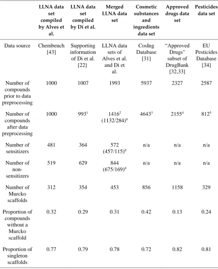
Whereas the data set compiled by Alves et al. is balanced (481 sensitizers; 519 non-sensitizers), the data set of Di et al. contains almost twice as many non-sensitizers (n = 629) as sensitizers (n = 364; Table 1). Roughly 40% of all compounds (567) are present in both data sets (Table 2). The LLNA data set compiled by Alves et al. contains 7% of all substances listed in the cosmetics data set; coverage is lower for approved drugs and pesticides (4% and 5%, respectively). The percentages are similar for the LLNA data set of Di et al.: 5% overlaps with cosmetics, 3% with approved drugs and 4% with pesticides. Merging the two LLNA data sets increases the number of unique compounds to 1416 and the overlaps with cosmetics, approved drugs and pesticides to 8%, 5% and 5%, respectively.
3.1.2. Coverage of Chemical Space
Table 1. Overview of all Data Sets Used in this Work.
LLNA data set compiled by Alves et
al.
LLNA data set compiled by Di et al.
Merged LLNA data set Cosmetic substances and ingredients data set Approved drugs data set Pesticides data set
Data source
Chembench
[43]
Supporting
information
of Di et al.
[22]
LLNA data
sets of
Alves et al.
and Di et
al.
CosIng
Database
[31]
“Approved
Drugs"
subset of
DrugBank
[32,33]
EU
Pesticides
Database
[34]
Number of
compounds
prior to data
preprocessing
1000
1007
1993
5937
2327
2587
Number of
compounds
after data
preprocessing
1000
993
11416
2(1132/284)
64643
32155
4812
5Number of
sensitizers
481
364
572
(457/115)
6n/a
n/a
n/a
Number of
non-sensitizers
519
629
844
(675/169)
6n/a
n/a
n/a
Number of
Murcko
scaffolds
312
354
453
856
1158
329
Proportion of
compounds
without a
Murcko
scaffold
0.32
0.29
0.31
0.42
0.13
0.24
Proportion of
singleton
scaffolds
0.77
0.79
0.78
0.72
0.82
0.81
1 Thirteen compounds were removed as part of the deduplication procedure; one compound was removed because of conflicting activity assignments.
2 Five hundred sixty-seven compounds were removed as part of the deduplication procedure; ten compounds were removed because of conflicting activity assignments.
3 One hundred four compounds were removed by the salt filter because the main component could not be unambiguously identified; 1190 compounds were removed as part of the deduplication procedure.
4 Thirty-one compounds were removed by the salt filter because the main component could not be unambiguously identified; 26 compounds were removed due to invalid input structure; 141 compounds were
5 Six compounds were removed by the salt filter because the main component could not be identified; 13 compounds were removed due to invalid input structure; 1756 compounds were removed as part of the
deduplication procedure.
6 Number of compounds in the training set/test set prior to descriptor calculation.
Table 2: Overlaps Between the Compounds Contained in the LLNA Data Sets and the Cosmetics, Approved Drugs and Pesticides Data Sets.
Number of
compounds
Data set compiled by
Alves et al.
Data set compiled
by Di et al.
Merged LLNA
data set
Cosmetics
4643
324
252
387
Approved
Drugs
2155
88
68
97
Pesticides
812
43
34
44
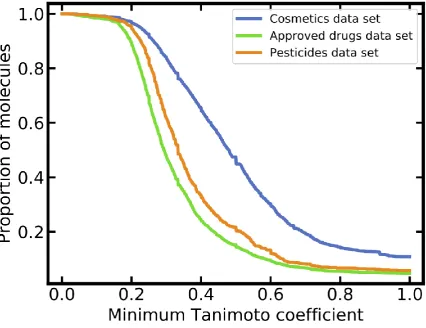
In addition to PCA analysis, the coverage of cosmetics, approved drugs and pesticides by the merged LLNA data set was quantified based on the distribution of maximum pairwise similarities. As shown in Figure 2, the merged LLNA data set covers cosmetics much better than approved drugs and pesticides: over 30% of all cosmetics are represented by the respective nearest neighbor in the merged LLNA data set with a minimum Tanimoto coefficient of 0.6, whereas this is the case for only 10% and 13% of all approved drugs and pesticides, respectively.
Figure 2. Molecular similarity between each compound of the reference data sets (i.e. cosmetics, approved drugs and pesticides data sets) and its nearest neighbor in the merged LLNA data set (similarity quantified as Tanimoto coefficient based on Morgan2 fingerprints with a length of 2048 bits).
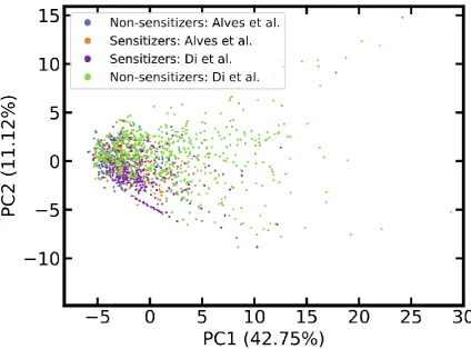
Figure 3. Score plot comparing the chemical space of compounds of the LLNA data sets of Alves et al. and Di et al. The score plot was derived from a PCA based on the identical setup described in the caption of Figure 1. Two data points are located outside the displayed intervals.
3.1.3. Molecular Diversity
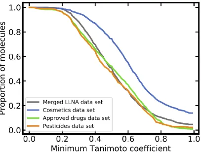
Figure 4. Pairwise molecular similarity within the individual data sets (similarity quantified as Tanimoto coefficient based on Morgan2 fingerprints with a length of 2048 bits).
The merged LLNA data set covers a total of 453 distinct Murcko scaffolds, which is roughly as many as covered by the pesticides data set but only one-third and one-quarter of those covered by the cosmetics and approved drugs data sets, respectively (Table 1). Taking into account the size of the individual data sets, the approved drugs data set clearly is the most diverse data set. In contrast, the cosmetics data set, which counts more molecular structures than all other data sets taken together, is the least diverse data set. This is in part related to the fact that approximately 40% of all cosmetics do not include a ring and, as such, do not have a Murcko scaffold.
Benzene is the most prominent Murcko scaffold across all data sets, with a prevalence of 27%, 28%, 10% and 23% among the merged LLNA, cosmetics, approved drugs and pesticides data sets. Any other scaffolds are represented by only a few instances (Table S2). Note the high percentages of singleton scaffolds (72% or higher) across all data sets, which, in particular in the case of the LLNA data set, illustrate the scarcity of the data available for modeling.
3.2. Molecular Properties of Skin Sensitizers and Non-sensitizers
Figure 5. PCA of the physicochemical properties of skin sensitizers and non-sensitizers included in the merged LLNA data set. The PCA is based on the identical setup described in the caption of Figure 1. (a) Score plot, with the percentage of variance explained by the individual principal components reported as part of the axis labels. Two data points are located outside the displayed intervals. (b) Loadings plot (an enlarged version is provided in Figure S1; the abbreviations of the individual molecular descriptors are explained in Table S1). (c) Detailed view of the lower left region of the score plot, where mainly sensitizers are observed to form a line of data points. These sensitizers are aliphatic, monohalogenated hydrocarbons that differ primarily by chain length and halogen atom type. (d) Detailed view of the upper right part of the score plot, where mainly non-sensitizing compounds are located, characterized by high molecular weight, aromaticity and a large topological polar surface area.
3.3. Model Development
Prior to model development, the merged LLNA data set was divided into a training (80%) and test (20%) set (Table 3; see Methods for details). All possible combinations of machine learning approaches (RF and SVM) with up to two different sets of molecular descriptors (including molecular fingerprints) were systematically explored (Table 4). One type of descriptors to highlight is a new fingerprint that we derive from the “Protein binding alerts for skin sensitization by OASIS” profiler implemented in the OECD toolbox. This profiler assigns compounds to eleven mechanistic domains associated with skin sensitization, five of which are represented by more than 20 instances in the training set (i.e. Michael addition, SN2 reaction, Schiff base formation, acylation, and nucleophilic
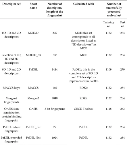
Table 3. Overview of Descriptor Sets Evaluated in this Work.
Descriptor set Short name
Number of descriptors/ length of the
fingerprint
Calculated with Number of
successfully processed molecules1
Training set
Test set
0D, 1D and 2D descriptors
MOE2D 206 MOE; this set
corresponds to all descriptors listed as “2D descriptors” in
MOE
1132 284
Selection of 0D, 1D and 2D descriptors
MOE2D_53 532 MOE 1132 284
0D, 1D and 2D descriptors
PaDEL 1444 PaDEL; this is the
complete set of 0D, 1D and 2D descriptors implemented in PaDEL
1109 279
MACCS keys MACCS 166 RDKit 1132 284
Morgan2 fingerprints
Morgan2 2048 RDKit 1132 284
OASIS skin sensitization protein binding
fingerprint
OASIS 5 bit fingerprint OECD Toolbox 1128 283
PaDEL estate fingerprint
PaDEL_Est 79 PaDEL 1132 284
PaDEL extended fingerprint
PaDEL_Ext 1024 PaDEL 1132 284
1 Descriptor calculation failed for individual compounds depending on the software used. For this reason there are marginal differences in the composition of the individual data sets used for model development.
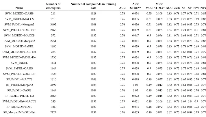
Table 4. Overview of Models and Their Performance During Cross-Validation.
1
Name
Number of descriptors
Number of compounds in training
data ACC
ACC
STDEV1 MCC
MCC
STDEV1AUC CCR Se SP PPV NPV
SVM_MOE2D+OASIS 211 1128 0.78 0.054 0.55 0.109 0.83 0.78 0.77 0.78 0.71 0.83
SVM_PaDEL+MACCS 1610 1108 0.76 0.035 0.51 0.069 0.83 0.76 0.75 0.76 0.69 0.82
SVM_PaDEL+Morgan2 3492 1108 0.76 0.036 0.51 0.078 0.82 0.75 0.66 0.83 0.73 0.78
SVM_PaDEL+PaDEL-Ext 2468 1109 0.76 0.039 0.51 0.075 0.84 0.76 0.74 0.78 0.7 0.81
SVM_MOE2D+MACCS 372 1132 0.76 0.047 0.5 0.096 0.81 0.74 0.68 0.81 0.71 0.79
SVM_MOE2D+Morgan2 2254 1132 0.75 0.041 0.5 0.081 0.83 0.75 0.77 0.73 0.66 0.83
SVM_MOE2D+PaDEL 1680 1109 0.76 0.039 0.5 0.079 0.83 0.75 0.74 0.77 0.69 0.81
SVM_MOE2D+PaDEL-Est 285 1132 0.76 0.039 0.5 0.081 0.81 0.75 0.68 0.81 0.71 0.79
SVM_MOE2D+PaDEL-Ext 1230 1132 0.75 0.054 0.5 0.105 0.83 0.75 0.75 0.76 0.68 0.81
SVM_PaDEL 1444 1109 0.75 0.038 0.5 0.075 0.83 0.75 0.75 0.75 0.68 0.81
SVM_PaDEL+OASIS 1449 1109 0.75 0.038 0.5 0.075 0.83 0.75 0.75 0.75 0.68 0.81
SVM_PaDEL+PaDEL-Est 1523 1109 0.75 0.038 0.5 0.075 0.83 0.75 0.75 0.75 0.68 0.81
RF_PaDEL+MACCS 1610 1108 0.76 0.018 0.49 0.037 0.82 0.73 0.62 0.85 0.74 0.77
RF_PaDEL+Morgan2 3492 1108 0.76 0.02 0.49 0.042 0.82 0.74 0.64 0.84 0.73 0.77
RF_PaDEL+OASIS 1449 1109 0.76 0.02 0.49 0.043 0.82 0.74 0.62 0.85 0.74 0.77
RF_PaDEL+PaDEL-Ext 2468 1109 0.76 0.022 0.49 0.048 0.82 0.73 0.61 0.86 0.75 0.76
SVM_PaDEL-Est+MACCS 245 1132 0.75 0.051 0.49 0.106 0.81 0.74 0.69 0.8 0.7 0.79
RF_MOE2D+PaDEL 1680 1109 0.75 0.034 0.48 0.072 0.83 0.73 0.62 0.84 0.73 0.77
RF_PaDEL 1444 1109 0.75 0.015 0.48 0.033 0.82 0.73 0.62 0.84 0.73 0.76
RF_PaDEL-Est+OASIS 84 1128 0.75 0.043 0.48 0.091 0.8 0.74 0.65 0.82 0.72 0.78
SVM_MACCS+OASIS 171 1128 0.75 0.047 0.48 0.102 0.82 0.74 0.69 0.79 0.69 0.79
SVM_MOE2D 206 1132 0.74 0.037 0.48 0.067 0.82 0.74 0.75 0.74 0.66 0.82
SVM_Morgan2+PaDEL-Ext 3072 1132 0.75 0.044 0.48 0.09 0.82 0.74 0.68 0.8 0.7 0.79
RF_MACCS 166 1132 0.75 0.039 0.47 0.088 0.81 0.73 0.61 0.84 0.73 0.76
RF_MACCS+OASIS 171 1128 0.75 0.034 0.47 0.074 0.8 0.73 0.6 0.85 0.74 0.76
RF_PaDEL+PaDEL-Est 1523 1109 0.75 0.028 0.47 0.06 0.83 0.73 0.61 0.85 0.73 0.76
SVM_MACCS 166 1132 0.74 0.057 0.47 0.12 0.81 0.73 0.69 0.78 0.68 0.79
SVM_PaDEL-Est+OASIS 84 1128 0.74 0.048 0.47 0.099 0.8 0.74 0.71 0.76 0.67 0.8
SVM_PaDEL-Est+PaDEL-Ext 1103 1132 0.74 0.039 0.47 0.08 0.81 0.74 0.7 0.78 0.68 0.79
SVM_PaDEL-Ext 1024 1132 0.74 0.046 0.47 0.093 0.81 0.73 0.7 0.77 0.68 0.79
SVM_PaDEL-Ext+OASIS 1029 1128 0.74 0.036 0.47 0.072 0.82 0.74 0.7 0.77 0.68 0.79
RF_MOE2D+Morgan2 2254 1132 0.74 0.033 0.46 0.071 0.81 0.72 0.62 0.82 0.71 0.76
RF_PaDEL-Est+MACCS 245 1132 0.75 0.045 0.46 0.1 0.81 0.72 0.59 0.85 0.73 0.76
RF_Morgan2 2048 1132 0.74 0.039 0.46 0.081 0.81 0.73 0.64 0.81 0.7 0.77
SVM_Morgan2+MACCS 2214 1132 0.74 0.058 0.46 0.117 0.8 0.73 0.68 0.78 0.68 0.78
SVM_PaDEL-Ext+MACCS 1190 1132 0.74 0.047 0.46 0.097 0.81 0.73 0.68 0.77 0.68 0.78
RF_MOE2D+OASIS 211 1128 0.74 0.041 0.45 0.09 0.81 0.71 0.6 0.83 0.71 0.75
RF_MOE2D+PaDEL-Est 285 1132 0.74 0.032 0.45 0.07 0.81 0.72 0.6 0.84 0.72 0.75
RF_MOE2D+PaDEL-Ext 1230 1132 0.74 0.017 0.45 0.037 0.82 0.72 0.58 0.85 0.73 0.75
RF_MOE2D+MACCS 372 1132 0.73 0.033 0.44 0.072 0.81 0.71 0.58 0.84 0.71 0.75
RF_Morgan2+MACCS 2214 1132 0.73 0.039 0.44 0.086 0.8 0.72 0.63 0.8 0.68 0.76
RF_Morgan2+OASIS 2053 1128 0.74 0.029 0.44 0.063 0.82 0.71 0.59 0.83 0.71 0.75
RF_Morgan2+PaDEL-Ext 3072 1132 0.73 0.036 0.44 0.081 0.81 0.71 0.56 0.85 0.72 0.74
SVM_MOE2D53 53 1132 0.71 0.037 0.44 0.069 0.78 0.72 0.76 0.68 0.62 0.81
SVM_PaDEL-Est 79 1132 0.72 0.037 0.44 0.073 0.77 0.72 0.71 0.73 0.64 0.79
RF_PaDEL-Est 79 1132 0.73 0.022 0.43 0.042 0.77 0.71 0.64 0.79 0.67 0.76
RF_PaDEL-Ext+MACCS 1190 1132 0.73 0.037 0.43 0.081 0.81 0.7 0.55 0.85 0.72 0.74
RF_PaDEL-Ext+OASIS 1029 1128 0.73 0.033 0.43 0.072 0.8 0.7 0.57 0.84 0.71 0.74
RF_PaDEL-Ext+PaDEL-Est 1103 1132 0.73 0.034 0.43 0.074 0.8 0.7 0.56 0.85 0.72 0.74
SVM_Morgan2+OASIS 2053 1128 0.73 0.038 0.43 0.089 0.8 0.69 0.51 0.88 0.75 0.73
SVM_Morgan2+PaDEL-Est 2127 1132 0.72 0.035 0.43 0.064 0.79 0.72 0.69 0.75 0.65 0.78
RF_MOE2D53 53 1132 0.73 0.039 0.42 0.086 0.78 0.7 0.58 0.83 0.69 0.74
RF_PaDEL-Ext 1024 1132 0.72 0.039 0.42 0.088 0.79 0.7 0.55 0.84 0.71 0.73
SVM_Morgan2 2048 1132 0.72 0.031 0.39 0.072 0.8 0.68 0.49 0.87 0.72 0.71
SVM_OASIS 5 1128 0.67 0.064 0.29 0.151 0.63 0.62 0.37 0.87 0.68 0.67
RF_OASIS 5 1128 0.66 0.054 0.27 0.122 0.64 0.63 0.43 0.82 0.62 0.68
1 Standard deviation.
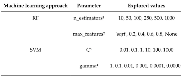
For any combination of machine learning algorithm and descriptor set(s), optimum hyperparameters were identified via a grid search (Table 5). The grid search was performed within the framework of a 10-fold cross-validation, with MCC used as the scoring parameter (see Methods for details). Note that MCC values range from -1 to +1. A value of +1 indicates perfect prediction, whereas a value of -1 indicates a prediction that is in total disagreement. A value of 0 indicates a performance which is equal to random.
The outcomes of this grid search are summarized in Table S3. It can be seen that similar hyperparameters tend to be selected by models based on related types and sets of molecular descriptors. No strong preferences for specific hyperparameter values are apparent. This is likely related to the fact that, within a broad value space, the hyperparameters only had a minor impact on model performance.
Table 5. Overview of Hyperparameters Optimized by Grid Search.
Machine learning approach Parameter Explored values
RF n_estimators1 10, 50, 100, 250, 500, 1000
max_features2 'sqrt', 0.2, 0.4, 0.6, 0.8, None
SVM C3 0.01, 0.1, 1, 10, 100, 1000
gamma4 1, 0.1, 0.01, 0.001, 0.0001, 0.00001
1 Number of prediction trees.
2 Maximum depth of each tree.
3 Penalty parameter C of the error term.
4 Coefficient for the radial basis function (rbf) kernel.
3.4. Model Performance
3.4.1. Model Performance During Cross-Validation
Depending on the combination of machine learning algorithm (RF or SVM) and descriptor set(s) used, MCC values ranged from 0.27 to 0.55, ACC values from 0.66 to 0.78, and AUC values from 0.63 to 0.84 (Table 4). The machine learning algorithms had only a minor impact on model performance. The average MCC values obtained by RFs and SVMs were 0.45 and 0.48, respectively. Nevertheless, the twelve predictors that obtained the highest MCC values are all based on SVMs. Most of the observed variation in performance stemmed from the use of different descriptor sets.
In most cases, the combination of two sets of molecular descriptors was beneficial to model performance. Exceptions include models based on combinations of two sets of descriptors of the same type (e.g. Morgan2 and MACCS fingerprints). These did not outperform the best models based on a single set of descriptors. Also combinations of 0D/1D/2D molecular descriptors with fingerprints did not consistently outperform models based on a single set of descriptors, albeit nine out of twelve models with MCC values greater than or equal to 0.5 are models combining non-binary molecular descriptors (i.e. MOE2D or PaDEL) with molecular fingerprints. Tables S4 and S5 provide a comprehensive overview of the impact of different combinations of descriptor sets on model performance.
Good performance was also obtained by models generated using non-commercial software only. For example, the SVM_PaDEL+OASIS model obtained MCC, ACC and AUC values of 0.50, 0.75 and 0.83, respectively. With few exceptions, the OASIS fingerprint contributed positively to the performance of models. For instance, adding the OASIS fingerprint to the SVM_MOE2D model led to an increase of the MCC, ACC and AUC by 0.07, 0.04 and 0.01, respectively. Interestingly, with a total of just 84 bits the RF_PaDEL-Est+OASIS model reached a level of performance that is comparable with that of more complex models (MCC 0.48; ACC 0.75; AUC 0.80). However, when used on its own, the OASIS fingerprint is not sufficient for good classification performance: the RF_OASIS and SVM_OASIS models obtained the lowest MCC values across all models (i.e. 0.27 and 0.29, respectively).
3.4.2. In-Depth Analysis of Selected Models within the Cross-Validation Framework
Based on the cross-validation results, five of the most interesting models were selected for additional studies:
• SVM_MOE2D+OASIS: the model with highest MCC
• SVM_PaDEL+OASIS: a model performing comparable to the SVM_MOE2D+OASIS and based on freely available software only
• SVM_PaDEL: the best model based on a single set of molecular descriptors • RF_MACCS: the best model based on a single set of molecular fingerprints
• SVM_PaDEL+MACCS: a model with good performance, combining the descriptor sets used by the above two models
Within the above-mentioned 10-fold cross-validation framework, we first analyzed how the coverage of the query molecules by the training data affects model performance. For this analysis we calculated the similarity between the individual query molecules and the one, three and five-nearest neighbors in the training set. Two similarity measures were explored: Tanimoto coefficients in the MACCS fingerprint space and negative Euclidean distances in the PaDEL descriptor space. The latter did not correlate well with molecular similarity (likely caused by noise related to the large number of molecular descriptors considered in this approach; Figure S2 and Table S6), for which reason we decided to go ahead with the fingerprint-based distance measure.
Figure 6. MCC as a function of molecular similarity between the query compounds and the one, three and five nearest neighbors in the training data (calculated as averaged Tanimoto coefficients based on MACCS fingerprints). (a) SVM_MOE2D+OASIS; (b) SVM_PaDEL+OASIS; (c) SVM_PaDEL; (d) RF_MACCS; (e) SVM_PaDEL+MACCS. Pearson’s correlation coefficients are reported in brackets in
Figure 7. MCC, sensitivity and specificity as a function of the decision threshold, for (a) SVM_MOE2D+OASIS; (b) SVM_PaDEL+OASIS; (c) SVM_PaDEL; (d) RF_MACCS; (e) SVM_PaDEL+MACCS. Note that different X-axis scales are applied to the graphs illustrating the performance of RF and SVM models.
RF_MACCS model, lowering the decision threshold to 0.3 results in a sensitivity of 0.84 and a specificity of 0.61 (Figure 7d).
Observing the predicted class probability can be of use for assessing the reliability of a prediction: as shown in Figure 8, the reliability of predictions increases with the absolute distance between the class probability and the decision threshold. For SVM models, predictions with class probabilities more than 0.5 away from the decision threshold had averaged MCC values between 0.63 and 0.67, whereas predictions with class probabilities less than 0.5 away had averaged MCC values of just 0.20 to 0.29. For the RF_MACCS model, predictions with class probabilities more than 0.35 away from the decision threshold had MCC values above 0.6, whereas predictions with class probabilities closer than 0.15 to the decision threshold had MCCs below 0.4. For the five investigated models the Pearson correlation coefficients for this relationship were between 0.92 and 0.98.
Figure 8. MCC as a function of the distance between the predicted class probabilities and the decision thresholds, for the (a) SVM models and (b) RF model. The number of compounds in each bin is summarized in Table S8.
As a further way of analyzing the data, we looked into the reliability of predictions as a function of the number of consecutive nearest neighbors in the training data that are of the same activity class as the one predicted for a compound of interest. From Figure 9 it can be seen that predictions are particularly reliable if the three nearest neighbors in the training data are of the identical class as the class predicted for a compound of interest. The strongest correlation is observed for the RF_MACCS model. For this model the MCC is close to zero for compounds where the predicted class is in conflict with the class assigned to the nearest neighbor. In contrast, the MCC is above 0.6 for compounds where the predicted class and the classes assigned to the three nearest neighbors are identical.
3.4.3. Performance of Selected Models on the Test Set
The performance of the five selected models was tested on holdout data. All models were stable, with only minor losses in MCC, ACC and AUC when compared to the results from cross-validation (Table 6). The largest losses in performance were observed for the RF_MACCS model, with MCC and ACC values decreased by 0.06 and 0.03, respectively (AUC however +0.01).
Defining the applicability domain with a cutoff of 0.50 rather than 0.75 led to only minor performance improvements compared to the model without applicability domain definition. This is related to the fact that only approximately 3% of the compounds of the test set are that dissimilar to the compounds in the training data. However, predictions for these compounds are unreliable (MCC values 0.2 or lower). Therefore it is important to observe the applicability domain of the individual models.
Figure 9. MCC as a function of the number of consecutive nearest neighbors in the training data that are of the same activity class as the predicted class for a compound of interest (molecular similarity quantified as Tanimoto coefficient based on MACCS fingerprints). The number of compounds in each bin is summarized in Table S9. The graphs for SVM_PaDEL+OASIS and SVM_PaDEL+MACCS are not shown because they are (almost) identical with that of SVM_PaDEL and would overlap.
Besides the applicability domain definition, users are advised to consider two additional types of information when judging the reliability of a prediction: (i) the distance between the predicted class probability from the decision threshold and (ii) the number of consecutive nearest neighbors that are of the same activity class than the class predicted for a compound of interest.
Larger distances of the class probability to the decision threshold indicate higher reliability of the prediction. For example, when considering only predictions with class probabilities 0.35 or further away from the decision threshold, the MCC of the RF_MACCS model increases from 0.41 to 0.78 (this covers 23% of the test set; Table 7). Likewise, for the SVM models MCC values increase from approximately 0.5 to a maximum of 0.78 when considering predictions only if their class probability is 1.25 or further away from the decision threshold (this covers 12% to 37% of the compounds in the test set).
Predictions for query molecules that are consistent with the class assigned to the k-nearest neighbors in the training data are more reliable than for those that are in conflict. This is also confirmed by the results obtained for the test set (Table 8): Predictions that are in disagreement with the activity class of the nearest neighbor resulted in MCC and ACC values no higher than 0.13 and 0.56, respectively. MCC and ACC values increase to a maximum of 0.98 and 0.99 when considering predictions only if they are consistent with three or more nearest neighbors.
Table 6. Performance of Selected Models on the Test Set.
Name
Mean Tanimoto
Number of
similarity to the five nearest neighbors
RF_MACCS 0 284 0.72 0.41 0.82 0.70 0.57 0.82 0.69 0.74
RF_MACCS ≥0.5 273 0.73 0.43 0.82 0.71 0.6 0.82 0.69 0.75
RF_MACCS ≥0.75 79 0.78 0.59 0.91 0.81 0.89 0.73 0.64 0.92
RF_MACCS <0.5 11 0.45 -0.29 0.60 0.42 0.00 0.83 0.00 0.50
SVM_MOE_2D+OASIS 0 283 0.76 0.52 0.83 0.76 0.81 0.72 0.66 0.85
SVM_MOE_2D+OASIS ≥0.5 273 0.76 0.53 0.84 0.77 0.82 0.72 0.67 0.86
SVM_MOE_2D+OASIS ≥0.75 79 0.81 0.64 0.89 0.84 0.93 0.75 0.67 0.95
SVM_MOE2D+OASIS <0.5 10 0.60 0.20 0.60 0.60 0.60 0.60 0.60 0.60
SVM_PaDEL 0 279 0.74 0.47 0.82 0.74 0.76 0.72 0.65 0.82
SVM_PaDEL ≥0.5 269 0.74 0.49 0.83 0.75 0.77 0.73 0.65 0.83
SVM_PaDEL ≥0.75 79 0.80 0.63 0.89 0.83 0.93 0.73 0.65 0.95
SVM_PaDEL <0.5 10 0.60 0.20 0.56 0.60 0.60 0.60 0.60 0.60
SVM_PaDEL+MACCS 0 279 0.75 0.50 0.82 0.75 0.78 0.73 0.66 0.83
SVM_PaDEL+MACCS ≥0.5 269 0.75 0.51 0.83 0.76 0.79 0.73 0.66 0.84
SVM_PaDEL+MACCS ≥0.75 79 0.80 0.63 0.89 0.83 0.93 0.73 0.65 0.95
SVM_PaDEL+MACCS <0.5 10 0.60 0.20 0.56 0.60 0.60 0.60 0.60 0.60
SVM_PaDEL+OASIS 0 279 0.74 0.48 0.82 0.74 0.76 0.73 0.65 0.82
SVM_PaDEL+OASIS ≥0.5 271 0.75 0.49 0.83 0.75 0.77 0.73 0.65 0.83
SVM_PaDEL+OASIS ≥0.75 79 0.80 0.63 0.89 0.83 0.93 0.73 0.65 0.95
SVM_PaDEL+OASIS <0.5 10 0.60 0.20 0.56 0.60 0.60 0.6 0.60 0.60
Table 7. Test Set Performance as a Function of the Distance of Predicted Class Probabilities from the Decision Threshold.
Name
Distance to decision threshold1
Number of
compounds ACC MCC AUC CCR Se Sp PPV NPV
RF-MACCS ≥0.15 175 0.85 0.67 0.46 0.84 0.81 0.87 0.76 0.90
RF-MACCS ≥0.35 66 0.91 0.78 0.42 0.89 0.85 0.93 0.85 0.93
RF-MACCS <0.15 109 0.51 0.04 0.42 0.52 0.32 0.72 0.55 0.50
SVM_MOE2D+OASIS ≥0.5 203 0.82 0.64 0.42 0.83 0.88 0.78 0.73 0.90
SVM_MOE2D+OASIS ≥1.25 106 0.89 0.76 0.41 0.89 0.89 0.88 0.81 0.94
SVM_MOE2D+OASIS <0.50 80 0.60 0.20 0.52 0.60 0.62 0.58 0.50 0.70
SVM_PaDEL ≥0.5 183 0.80 0.61 0.48 0.81 0.86 0.76 0.71 0.89
SVM_PaDEL <0.50 96 0.61 0.21 0.36 0.60 0.55 0.66 0.51 0.69
SVM_PaDEL+MACCS ≥0.5 183 0.80 0.62 0.49 0.82 0.88 0.75 0.71 0.90
SVM_PaDEL+MACCS ≥1.25 37 0.86 0.75 0.52 0.9 1.00 0.80 0.71 1.00
SVM_PaDEL+MACCS <0.50 96 0.65 0.27 0.39 0.63 0.58 0.69 0.55 0.71
SVM_PaDEL+OASIS ≥0.5 183 0.80 0.61 0.49 0.81 0.86 0.76 0.71 0.89
SVM_PaDEL+OASIS ≥1.25 34 0.88 0.78 0.45 0.91 1.00 0.82 0.75 1.00
SVM_PaDEL+OASIS <0.50 96 0.62 0.22 0.37 0.61 0.55 0.67 0.52 0.70
1
Distance of predicted class probabilities from the decision threshold
Table 8. Test Set Performance as a Function of the Number of Consecutive Nearest Neighbors with Class Assignments Consistent with the Predicted Class.
Name
Number of concordant neighbors1
Number of
compounds ACC MCC AUC CCR Se Sp PPV NPV
RF_MACCS 0 87 0.33 -0.35 0.32 0.33 0.19 0.48 0.26 0.38
RF_MACCS ≥1 197 0.89 0.77 0.97 0.87 0.81 0.94 0.89 0.89
RF_MACCS ≥2 147 0.96 0.90 1.00 0.94 0.89 0.99 0.98 0.95
RF_MACCS ≥3 113 0.99 0.98 1.00 0.98 0.97 1.00 1.00 0.99
SVM_MOE2D+OASIS 0 85 0.56 0.13 0.56 0.57 0.62 0.51 0.55 0.58
SVM_MOE2D+OASIS ≥1 198 0.84 0.69 0.94 0.85 0.92 0.79 0.72 0.94
SVM_MOE2D+OASIS ≥2 146 0.91 0.81 0.99 0.92 0.95 0.89 0.79 0.98
SVM_MOE2D+OASIS ≥3 115 0.91 0.80 0.99 0.92 0.94 0.90 0.79 0.97
SVM_PaDEL 0 86 0.53 0.07 0.52 0.54 0.56 0.51 0.51 0.56
SVM_PaDEL ≥1 193 0.83 0.66 0.92 0.84 0.87 0.8 0.72 0.92
SVM_PaDEL ≥2 147 0.89 0.78 0.96 0.91 0.96 0.86 0.76 0.98
SVM_PaDEL ≥3 113 0.90 0.79 0.97 0.92 0.97 0.88 0.76 0.99
SVM_PaDEL+MACCS 0 86 0.55 0.10 0.53 0.55 0.59 0.51 0.52 0.57
SVM_PaDEL+MACCS ≥1 193 0.84 0.68 0.91 0.85 0.89 0.81 0.73 0.93
SVM_PaDEL+MACCS ≥2 147 0.90 0.80 0.96 0.92 0.96 0.88 0.79 0.98
SVM_PaDEL+MACCS ≥3 113 0.91 0.81 0.97 0.93 0.97 0.89 0.78 0.99
SVM_PaDEL+OASIS 0 86 0.53 0.07 0.52 0.54 0.56 0.51 0.51 0.56
SVM_PaDEL+OASIS ≥1 193 0.83 0.67 0.92 0.84 0.87 0.81 0.73 0.92
SVM_PaDEL+OASIS ≥2 147 0.9 0.79 0.96 0.91 0.96 0.87 0.77 0.98
SVM_PaDEL+OASIS ≥3 113 0.91 0.81 0.97 0.93 0.97 0.89 0.78 0.99
1 Number of consecutive nearest neighbors in the training data having the same activity class assigned as the one predicted
3.4.4. Comparison of Model Performance to that of Existing Models
Major caveats must be considered when attempting to directly compare the performance reported for existing models with those presented in this work. Not only do the underlying training and test sets differ substantially, but also the protocols used for performance evaluation and the definitions of the models’ applicability domains. Roughly summarized, Alves et al. reported their predictor of binary LLNA outcomes to yield a CCR of 0.77 during external cross-validation [28]. Di et al. reported their best global model for the binary prediction of LLNA outcomes, a SVM model based on PaDEL-Ext descriptors (Ext-SVM), to have yielded an ACC of 0.84 during cross-validation and an ACC of 0.81 on their test set (when considering the applicability domain according to their definition) [22]. In comparison, our best model (SVM_MOE2D+OASIS) yielded a CCR of 0.78 and identical ACC during cross-validation (MCC 0.55), without consideration of the applicability domain. On the test set, the SVM_MOE2D+OASIS model obtained a CCR of 0.76 and an MCC of 0.52. In this case, the consideration of the applicability domain of the model (defined as including any compound with a mean Tanimoto similarity to the five nearest neighbors in the training set of 0.50 or higher) did not yield a further improvement of performance. The SVM_PaDEL and RF_MACCS models, which are available via a public web service, yielded comparable CCR values (0.74 and 0.70 without consideration of the applicability domain; 0.75 and 0.71 with consideration of the applicability domain, respectively). The latter model has the additional benefit of being based on a fingerprint with a length of only 166 bits.
3.5. Skin Doctor Web Service
The final RF_MACCS and SVM_PaDEL models, trained not on the cross-validation data set but on the complete, preprocessed data set (1416 and 1388 compounds, depending on the number of compounds for which descriptors could be successfully calculated) are provided via the New E-Resource for Drug Discovery (NERDD)
[44]. Queries can either be directly drawn or uploaded in
different formats. Users may change the default decision threshold to steer the model's sensitivity and specificity. Results are presented in a tabular overview and can be exported as a CSV file. For each query they include information on (i) whether or not the query is within the applicability domain of the model, (ii) the predicted activity classes, (iii) distances from the selected decision threshold, (iv) mean similarity between the query compound and the five-nearest neighbors of the training set and (v) number of consecutive nearest neighbors in the training data of which the activity label is consistent with that of the prediction. The analysis and visualization of the corresponding effects presented in this work may be used as guidance to choose the required confidence in the prediction, being aware of the corresponding effects on the model's applicability domain and the requirements for similarity.Predictions are flagged with reliability warnings (a) if the mean similarity between the compound of interest and the five nearest neighbors is less than 0.5, or (b) if the predictions are in conflict with the activity of the nearest neighbor in the training data, or (c) if the distance to the decision threshold is small (0.15 for the RF_MACCS model; 0.5 for the SVM_PaDEL model).
Conclusions
An interesting observation to make was that a cluster of skin sensitizers and non-sensitizers with long aliphatic and halogenated chains could only be discriminated in the "MOE 2D" descriptor space but not in the Morgan2 fingerprint space, which should be taken into consideration for model building. The best models derived from the new LLNA data set obtained MCC and ACC values of up to 0.55 and 0.78 during cross-validation and of up to 0.52 and 0.76 on holdout data, respectively. Importantly, some of the models based entirely on free software and/or molecular descriptors of low complexity yielded comparable performance. We identified the RF_MACCS and SVM_PaDEL models as our favorite models, yielding MCC values of 0.41 and 0.47 on the holdout data. Comparison to existing models indicates that our models reach competitive performance. They are trained on a data set consisting of almost 3.5 times as many compounds as the one used by Di et al. The full data set used for modeling and testing is also 42% larger than that of Alves et al. Given the fact that the data set compiled by Di et al. holds in particular a diverse set of non-sensitizers not covered by Alves et al., we expect that our models, as they are based on the amalgamated data set, are more widely applicable and more reliable.
A major aspect of this work is the definition of an applicability domain for the individual models and the elaboration of means to estimate the reliability of predictions. The applicability domain was defined based on the mean similarity of a compound of interest to the five-nearest neighbors in the training data (quantified in MACCS fingerprint space). The difference between the predicted class probability and the decision threshold, as well as the number of consecutive nearest neighbors in the training data having the same activity class assigned as the one predicted for the compound of interest proved to be useful indicators of the reliability of predictions. We recommend to consider predictions as reliable if all of the following conditions are met:
• The compound of interest is within the applicability domain of the model.
• The distance between the predicted class probability and the decision threshold is at least 0.15 for RF models and 0.5 for SVM models.
• The predicted activity class for a compound of interest is in agreement with the class assigned to the nearest neighbor in the training data.
The public web service, available at https://nerdd.zbh.uni-hamburg.de/skinDoctor/, provides access to the final RF_MACCS and SVM_PaDEL models (i.e. models trained on the complete LLNA data set). Users are provided detailed information on whether or not a compound of interest fulfills the three criteria itemized above. A warning is issued in case predictions are determined to be unreliable. Users may also adjust the decision threshold, allowing them, e.g., to increase the model’s sensitivity in scenarios where it is desirable to flag even substances with a low likelihood of being skin sensitizers.
We hope that the models will be well received by the scientific community and will make a contribution to the development and application of non-animal methods for the prediction of the skin sensitization potential of small organic molecules.
Supplementary Materials: Supplementary materials can be found at https://www.preprints.org/manuscript/201908.0302/.
Author Contributions: Conceptualization, A.W., J.Kü. and J.Ki.; Methodology, A.W., C.S., C.B., J.Kü. and J.Ki.; Software, A.W. and C.S.; Validation, A.W.; Formal Analysis, A.W.; Investigation, A.W., C.S., C.B., J.Kü. and J.Ki; Resources, A.S., J.Kü. and J.Ki.; Data Curation, A.W.; Writing – Original Draft Preparation, A.W., C.S., C.B., A.S., J.Kü. and J.Ki.; Writing – Review & Editing, n/a; Visualization, A.W.; Supervision, A.S., J.Kü. and J.Ki.; Project Administration, J.Kü and J.Ki.; Funding Acquisition, A.S., J.Kü. and J.Ki.
Funding: A.W. is supported by Beiersdorf AG through HITeC e.V. C.B. and J.Ki. are supported by the Bergen Research Foundation (BFS) [BFS2017TMT01].
Abbreviations
ACC accuracy
ACD allergic contact dermatitis
AUC area under the receiver operating characteristic curve CCR correct classification rate
LLNA local lymph node assay
MCC Matthews correlation coefficients MOE Molecular Operating Environment NERDD New E-Resource for Drug Discovery NPV negative predictive value
PCA principal component analysis RBF radial basis function
RF random forest
PPV positive predictive value Se sensitivity
Sp specificity
SVM support vector machine
References
1.
Kimber, I.; Basketter, D.A.; Gerberick, G.F.; Ryan, C.A.; Dearman, R.J. Chemical allergy:
translating biology into hazard characterization.
Toxicol. Sci.
2011
,
120 Suppl 1
, S238–S268.
2.
Thyssen, J.P.; Linneberg, A.; Menné, T.; Johansen, J.D. The epidemiology of contact allergy in
the general population – prevalence and main findings.
Contact Derm.
2007
,
57
, 287–299.
3.
Lushniak, B.D. Occupational contact dermatitis.
Dermatol. Ther.
2004
,
17
, 272–277.
4.
Anderson, S.E.; Siegel, P.D.; Meade, B.J. The LLNA: a brief review of recent advances and
limitations.
J. Allergy
2011
,
2011
, 424203.
5.
Dent, M.; Amaral, R.T.; Da Silva, P.A.; Ansell, J.; Boisleve, F.; Hatao, M.; Hirose, A.; Kasai,
Y.; Kern, P.; Kreiling, R.; et al. Principles underpinning the use of new methodologies in the risk
assessment of cosmetic ingredients.
Computational Toxicology
2018
,
7
, 20–26.
6.
Mehling, A.; Eriksson, T.; Eltze, T.; Kolle, S.; Ramirez, T.; Teubner, W.; van Ravenzwaay, B.;
Landsiedel, R. Non-animal test methods for predicting skin sensitization potentials.
Arch.
Toxicol.
2012
,
86
, 1273–1295.
7.
Reisinger, K.; Hoffmann, S.; Alépée, N.; Ashikaga, T.; Barroso, J.; Elcombe, C.; Gellatly, N.;
Galbiati, V.; Gibbs, S.; Groux, H.; et al. Systematic evaluation of non-animal test methods for
skin sensitisation safety assessment.
Toxicol. In Vitro
2015
,
29
, 259–270.
8.
Ezendam, J.; Braakhuis, H.M.; Vandebriel, R.J. State of the art in non-animal approaches for
skin sensitization testing: from individual test methods towards testing strategies.
Arch. Toxicol.
2016
,
90
, 2861–2883.
9.
Thyssen, J.P.; Giménez-Arnau, E.; Lepoittevin, J.-P.; Menné, T.; Boman, A.; Schnuch, A. The
critical review of methodologies and approaches to assess the inherent skin sensitization
potential (skin allergies) of chemicals. Part I.
Contact Derm.
2012
,
66 Suppl 1
, 11–24.
10.
Wilm, A.; Kühnl, J.; Kirchmair, J. Computational approaches for skin sensitization prediction.
Crit. Rev. Toxicol.
2018
,
48
, 738–760.
11.
ECHA (European Chemicals Agency) The use of alternatives to testing on animals for the
REACH regulation, third report under article 117(3) of the REACH regulation Available online:
https://echa.europa.eu/documents/10162/13639/alternatives_test_animals_2017_en.pdf
(accessed on Jul 10, 2019).
12.
Kleinstreuer, N.C.; Hoffmann, S.; Alépée, N.; Allen, D.; Ashikaga, T.; Casey, W.; Clouet, E.;
Cluzel, M.; Desprez, B.; Gellatly, N.; et al. Non-animal methods to predict skin sensitization (II):
an assessment of defined approaches.
Crit. Rev. Toxicol.
2018
,
48
, 359–374.
13.
Luechtefeld, T.; Marsh, D.; Rowlands, C.; Hartung, T. Machine learning of toxicological big
14.
Luechtefeld, T.; Rowlands, C.; Hartung, T. Big-data and machine learning to revamp
computational toxicology and its use in risk assessment.
Toxicol. Res.
2018
,
7
, 732–744.
15.
Alves, V.M.; Borba, J.; Capuzzi, S.J.; Muratov, E.; Andrade, C.H.; Rusyn, I.; Tropsha, A. Oy
vey! A comment on “Machine learning of toxicological big data enables read-across structure
activity relationships outperforming animal test reproducibility.”
Toxicol. Sci.
2019
,
167
, 3–4.
16.
Luechtefeld, T.; Marsh, D.; Hartung, T. Missing the difference between big data and artificial
intelligence in RASAR versus traditional QSAR.
Toxicol. Sci.
2019
,
167
, 4–5.
17.
Tung, C.-W.; Lin, Y.-H.; Wang, S.-S. Transfer learning for predicting human skin sensitizers.
Arch. Toxicol.
2019
,
93
, 931–940.
18.
Chilton, M.L.; Macmillan, D.S.; Steger-Hartmann, T.; Hillegass, J.; Bellion, P.; Vuorinen, A.;
Etter, S.; Smith, B.P.C.; White, A.; Sterchele, P.; et al. Making reliable negative predictions of
human skin sensitisation using an in silico fragmentation approach.
Regul. Toxicol. Pharm.
2018
,
95
, 227–235.
19.
Braga, R.C.; Alves, V.M.; Muratov, E.N.; Strickland, J.; Kleinstreuer, N.; Trospsha, A.; Andrade,
C.H. Pred-Skin: a fast and reliable web application to assess skin sensitization effect of chemicals.
J. Chem. Inf. Model.
2017
,
57
, 1013–1017.
20.
Kim, J.Y.; Kim, M.K.; Kim, K.-B.; Kim, H.S.; Lee, B.-M. Quantitative structure–activity and
quantitative structure–property relationship approaches as alternative skin sensitization risk
assessment methods.
J. Toxicol. Environ. Health
2019
,
82
, 447–472.
21.
Toropov, A.A.; Toropova, A.P.; Selvestrel, G.; Benfenati, E. Idealization of correlations between
optimal simplified molecular input-line entry system-based descriptors and skin sensitization.
SAR QSAR Environ. Res.
2019
,
30
, 447–455.
22.
Di, P.; Yin, Y.; Jiang, C.; Cai, Y.; Li, W.; Tang, Y.; Liu, G. Prediction of the skin sensitising
potential and potency of compounds via mechanism-based binary and ternary classification
models.
Toxicol. In Vitro
2019
,
59
, 204–214.
23.
Alves, V.M.; Muratov, E.; Fourches, D.; Strickland, J.; Kleinstreuer, N.; Andrade, C.H.; Tropsha,
A. Predicting chemically-induced skin reactions. Part I: QSAR models of skin sensitization and
their application to identify potentially hazardous compounds.
Toxicol. Appl. Pharmacol.
2015
,
284
, 262–272.
24.
Lu, J.; Zheng, M.; Wang, Y.; Shen, Q.; Luo, X.; Jiang, H.; Chen, K. Fragment-based prediction
of skin sensitization using recursive partitioning.
J. Comput.-Aided Mol. Des.
2011
,
25
, 885–893.
25.
Chaudhry, Q.; Piclin, N.; Cotterill, J.; Pintore, M.; Price, N.R.; Chrétien, J.R.; Roncaglioni, A.
Global QSAR models of skin sensitisers for regulatory purposes.
Chem. Cent. J.
2010
,
4
, S5.
26.
Enoch, S.J.; Roberts, D.W. Predicting skin sensitization potency for Michael acceptors in the
LLNA using quantum mechanics calculations.
Chem. Res. Toxicol.
2013
,
26
, 767–774.
27.
Hoffmann, S. LLNA variability: an essential ingredient for a comprehensive assessment of
non-animal skin sensitization test methods and strategies.
ALTEX
2015
,
32
, 379–383.
28.
Alves, V.M.; Capuzzi, S.J.; Braga, R.C.; Borba, J.V.B.; Silva, A.C.; Luechtefeld, T.; Hartung,
T.; Andrade, C.H.; Muratov, E.N.; Tropsha, A. A perspective and a new integrated
computational strategy for skin sensitization assessment.
ACS Sustain. Chem. Eng.
2018
,
6
,
2845–2859.
29.
Apt Systemst Ltd. http://aptsys.net QSAR Toolbox 4.3 Available online:
http://oasis-lmc.org/products/software/toolbox.aspx (accessed on Jul 10, 2019).
30.
Chembench | Home Available online: https://chembench.mml.unc.edu (accessed on Apr 26,
2019).
31.
CosIng
- Cosmetics - GROWTH - European Commission Available online:
http://ec.europa.eu/growth/tools-databases/cosing/index.cfm?fuseaction=search.simple
(accessed on Apr 26, 2019).
32.
DrugBank Version 5.1.2 Available online: https://www.drugbank.ca (accessed on May 7, 2019).
33.
Wishart, D.S.; Feunang, Y.D.; Guo, A.C.; Lo, E.J.; Marcu, A.; Grant, J.R.; Sajed, T.; Johnson,
D.; Li, C.; Sayeeda, Z.; et al. DrugBank 5.0: a major update to the DrugBank database for 2018.
34.
EU
Pesticides
database
-
European
Commission
Available
online:
http://ec.europa.eu/food/plant/pesticides/eu-pesticides-database/public/?event=activesubstance.selection&language=EN (accessed on Feb 25, 2019).
35.
Stork, C.; Wagner, J.; Friedrich, N.-O.; de Bruyn Kops, C.; Šícho, M.; Kirchmair, J. Hit Dexter:
A machine-learning model for the prediction of frequent hitters.
ChemMedChem
2018
,
13
, 564–
571.
36.
MolVs Available online: MolVs version 0.1.1. https://github.com/mcs07/MolVS (accessed on
Apr 26, 2019).
37.
Chemical Computing Group Molecular Operating Environment (MOE) | MOEsaic | PSILO
Available online: https://www.chemcomp.com/Products.htm (accessed on Jun 12, 2019).
38.
Landrum, G. RDKit Available online: http://www.rdkit.org (accessed on Apr 26, 2019).
39.
PaDEL-Descriptor Available online: http://www.yapcwsoft.com/dd/padeldescriptor/ (accessed
on May 10, 2019).
40.
Yap, C.W. PaDEL-descriptor: an open source software to calculate molecular descriptors and
fingerprints.
J. Comput. Chem.
2011
,
32
, 1466–1474.
41.
scikit-learn: machine learning in Python — scikit-learn 0.21.0 documentation Available online:
https://scikit-learn.org/stable/ (accessed on May 10, 2019).
42.
Matthews, B.W. Comparison of the predicted and observed secondary structure of T4 phage
lysozyme.
Biochim. Biophys. Acta, Protein Struct.
1975
,
405
, 442–451.
43.