Flows in Vibrating Channels

(1)

Scholarship@Western

Electronic Thesis and Dissertation Repository

9-24-2015 12:00 AM

Flows in Vibrating Channels

Sahab Zandi

The University of Western Ontario

Supervisor

Dr. Jerzy Maciej Floryan

The University of Western Ontario

Graduate Program in Mechanical and Materials Engineering

A thesis submitted in partial fulfillment of the requirements for the degree in Master of Engineering Science

Follow this and additional works at: https://ir.lib.uwo.ca/etd

Part of the Mechanical Engineering Commons

Recommended Citation Recommended Citation

Zandi, Sahab, "Flows in Vibrating Channels" (2015). Electronic Thesis and Dissertation Repository. 3250.

https://ir.lib.uwo.ca/etd/3250

This Dissertation/Thesis is brought to you for free and open access by Scholarship@Western. It has been accepted for inclusion in Electronic Thesis and Dissertation Repository by an authorized administrator of

(2)

(Thesis format: Monograph)

by

Sahab Zandi

Graduate Program in Mechanical and Materials Engineering

A thesis submitted in partial fulfillment of the requirements for the degree of

Master of Engineering Science

The School of Graduate and Postdoctoral Studies The University of Western Ontario

London, Ontario, Canada

(3)

ii

Abstract

A spectral algorithm based on the immersed boundary conditions (IBC) concept has been

developed for the analysis of flows in channels bounded by vibrating walls. The vibrations

take the form of travelling waves of arbitrary profile. The algorithm uses a fixed

computational domain with the flow domain immersed in its interior. Boundary conditions

enter the algorithm in the form of constraints. The spatial discretization uses a Fourier

expansion in the stream-wise direction and a Chebyshev expansion in the wall-normal

direction. Use of the Galileo transformation converts the unsteady problem into a steady one.

An efficient solver which takes advantage of the structure of the coefficient matrix has been

used. It is demonstrated that the method can be extended to more extreme geometries using

the over-determined formulation. Various tests confirm the spectral accuracy of the

algorithm. Pressure losses in these types of channels have been analyzed. Mechanisms of

drag generation have been studied. Analytical solutions have been determined in the limit of

long wavelength waves and small amplitude waves in order to simplify identification of these

mechanisms. The numerical algorithm has also been validated with the help of analytical

solutions. Detailed analyses of different cases, i.e. wave propagation along one wall and both

walls have been carried out. Different wave profiles have been considered in order to find

forms of waves which minimize pressure losses in vibrating channels. The results show

dependence of the pressure losses on the phase speed of the waves, with the waves

propagating in the downstream direction reducing the pressure gradient required to maintain

a fixed flow rate. A drag increase is observed when the waves propagate with a phase speed

similar to the flow velocity.

Keywords

Spectral discretization, vibrating walls, immersed boundary conditions method,

Navier-Stokes equations, pressure-driven flows, efficient solvers, over-determined formulation,

(4)

iii

Co-Authorship Statement

This dissertation is prepared in the monograph format. Sections 2, 3, and 4 are based on

manuscripts that have been previously published or finalized for submission.

Sections 2 and 3: S. Zandi, A. Mohammadi & J. M. Floryan, “Spectrally-Accurate

Algorithm for the Analysis of Flows in Two-Dimensional Vibrating Channels”, Journal of

Computational Physics 301 (2015) 425–455, DOI: 10.1016/j.jcp.2015.08.025.

Section 4: S. Zandi & J. M. Floryan, “Pressure Losses in Vibrating Channels”, in preparation

(5)

iv

Dedication

(6)

v

Acknowledgments

It is a pleasure to thank the many people who made this thesis possible. I greatly appreciate

the unparalleled assistance and encouragement of my supervisor Prof. J. M. Floryan. The

completion of this dissertation would not have been possible without his incomparable

assistance and invaluable guidance.

I would like to express my gratitude to the members of my advisory committee, Prof. C.

Zhang and Prof. A. G. Straatman for their invaluable suggestions and constructive comments.

I would also like to thank all of my colleagues (past and present), Dr. Alireza Mohammadi,

Dr. Hadi Vafadar Moradi, Md Nazmus Sakib, Amirreza Seddighi, Seyed Arman Abtahi and

Alan Kalbfleisch for their friendship and encouragement. I am particularly grateful to Alireza

not only for his insightful scientific comments but also because of support and motivation I

have received from him.

Words are not enough to express my gratitude towards my family. Without the unconditional

love, encouragement, tremendous patience and understanding of parents, Soheila and

Masoud, and my sister, Saghar, I would not have been able to accomplish my goals. I wish I

could show them how much I love and appreciate them.

Finally I would like to mention that the support from The University of Western Ontario and

the Natural Sciences and Engineering Research Council (NSERC) of Canada is gratefully

(7)

vi

List of Figures

Figure 2.1: Sketch of the flow domain. ... 7

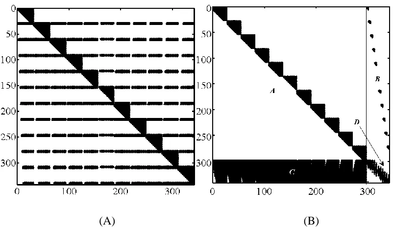
Figure 3.1: Structure of the coefficient matrix 𝐿 for 𝑁_𝑀 = 5 and 𝑁_𝑇 = 31. Black identifies

the non-zero elements. Figure 3.1A displays the coefficient matrix before the re-arrangement

whereas Figure 3.1B displays its structure after the re-arrangement (see Subsection 3.6). .. 28

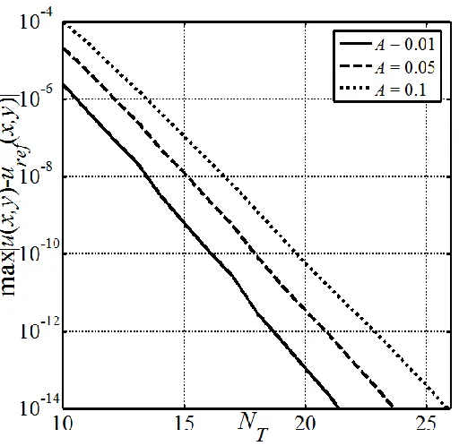
Figure 3.2: Variations of the error 𝐸𝑟 (see Eq. (3.65)) for the wave shape described by Eq.

(3.64) with the wave number = 1, Reynolds number 𝑅𝑒 = 5, phase speed 𝑐 = 1.3 and wave amplitudes 𝐴 shown on the graph. ... 30

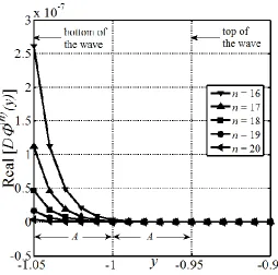
Figure 3.3: Distribution of the real part of 𝐷Ф(𝑛) as a function of 𝑦 for higher Fourier modes

(𝑛 > 15) in the region very close to the lower wall for the wave shape described by Eq.

(3.64) with the wave number  = 5, amplitude 𝐴 = 0.05, Reynolds number 𝑅𝑒 = 5 and phase speed 𝑐 = 1.3 obtained using 𝑁_𝑀 = 20 Fourier modes and 𝑁_𝑇 = 80 Chebyshev

polynomials. .... ... 31

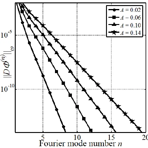
Figure 3.4: Variations of the Chebyshev norm of 𝐷Ф(𝑛) as a function of the Fourier mode

number determined for the wave shape described by Eq. (3.64) with the wave number = 1

and with different wave amplitudes 𝐴. Calculations were carried out for Reynolds number

𝑅𝑒 = 5 and wave phase speed 𝑐 = 1.3 using 𝑁𝑀 = 20 Fourier modes and 𝑁𝑇 = 80

Chebyshev polynomials. .... ... 32

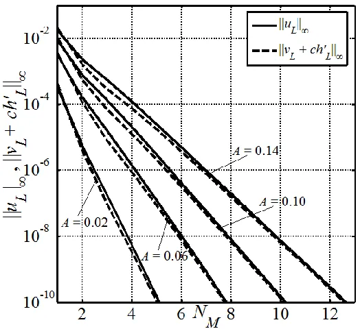
Figure 3.5: Variations of the ‖𝑢𝐿‖∞, ‖𝑣𝐿+ 𝑐ℎ𝐿′‖∞ norms as functions of the total number of

Fourier modes 𝑁_𝑀 used in the calculation for the wave shape described by Eq. (3.64) with the

wave number = 1 and with different amplitudes 𝐴. Calculations have been carried out for Reynolds number 𝑅𝑒 = 5 and phase speed 𝑐 = 1.3 using 𝑁_𝑇 = 80 Chebyshev polynomials.

... 33

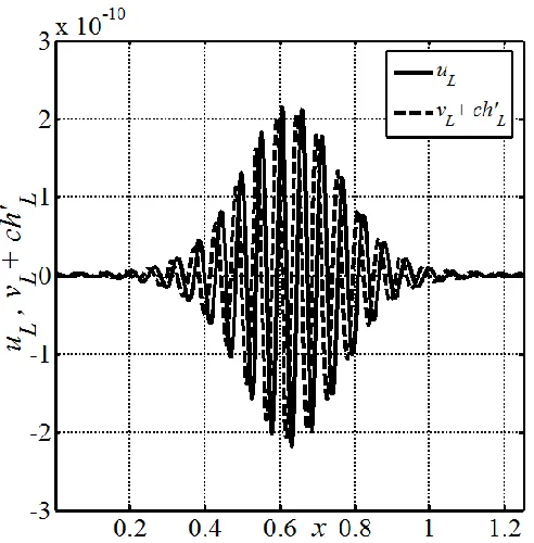
Figure 3.6: Distributions of the error in the enforcement of the boundary conditions along

the vibrating wall, i.e. 𝑢_𝐿 and 𝑣_𝐿+ 𝑐ℎ_𝐿′_{, for the wave with shape described by Eq. (3.64) with}

(10)

ix

𝑅𝑒 = 5 𝑐 = 1.3 𝑁𝑀 = 20 𝑁𝑇 = 80

Chebyshev polynomials. ... 34

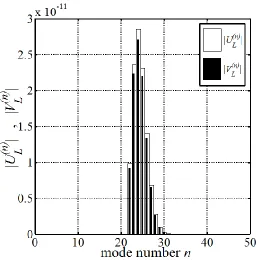
Figure 3.7: Fourier spectra of the error in the enforcement of the boundary conditions along

the vibrating wall, i.e. Eq. (3.68), for the wave with shape described by Eq. (3.64) with wave

number = 5 and amplitude 𝐴 = 0.05. Calculations were carried out for the Reynolds number 𝑅𝑒 = 5 and phase speed 𝑐 = 1.3 using 𝑁_𝑀 = 20 Fourier modes and 𝑁_𝑇 = 80

Chebyshev polynomials. The reader should note the absence of the first 20 Fourier modes. 35

Figure 3.8: Fourier spectra of 𝑢𝐿(𝑥) for the wave shape described by Eq. (3.64) with the

amplitude 𝐴 = 0.04 and wavelength 𝜆_𝑥= 2𝜋/3. Solutions have been obtained in case A

using 𝑁_𝑀 = 10 Fourier modes, in case B using 𝑁_𝑀 = 20 Fourier modes, and in case C using

𝑁𝑀 = 30 Fourier modes. Calculations were carried out with Reynolds number 𝑅𝑒 = 5 and

phase speed 𝑐 = 1.3 using 𝑁_𝑇 = 80 Chebyshev polynomials. ... 36

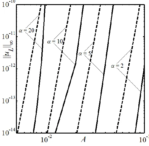
Figure 3.9: Variations of the ‖𝑢_𝐿‖_∞ norm for the wave shape described by Eq. (3.64) as a

function of the wave amplitude 𝐴 for selected wave numbers . Dashed and solid lines correspond to results obtained with 𝑁_𝑀 = 15 and 𝑁_𝑀 = 20 Fourier modes, respectively.

Calculations have been carried out for the Reynolds number 𝑅𝑒 = 5 and phase speed 𝑐 = 1.3

using 𝑁𝑇 = 80 Chebyshev polynomials. ... 37

Figure 3.10: Variations of the ‖𝑢𝐿‖∞ norm for the wave shape described by Eq. (3.64)as a

function of the wave number  for selected amplitudes 𝐴. Dashed and solid lines correspond to results obtained with 𝑁𝑀 = 15 and 𝑁𝑀 = 20 Fourier modes, respectively. Calculations

have been carried out with Reynolds number 𝑅𝑒 = 5 and phase speed 𝑐 = 1.3 using 𝑁_𝑇 =

80 Chebyshev polynomials. ... 38

Figure 3.11: Variations of the ‖𝑢𝐿‖∞ norm for the wave shape described by Eq. (3.64) with

the wave number = 2, the amplitude 𝐴 = 0.06 and the phase speed 𝑐 = 1.3 as a function of Reynolds number computed using different numbers of Fourier modes 𝑁_𝑀 and 𝑁_𝑇 = 80

Figure 3.12: Variations of the ‖𝑢𝐿‖∞ norm for the wave shape described by Eq. (3.64) with

(11)

x

phase speed 𝑐 determined using different numbers of Fourier modes 𝑁𝑀 and 𝑁𝑇 = 80

Figure 3.13: Structure of the coefficient matrix 𝐿₀ for 𝑁_𝑀 = 5, 𝑀_𝑀 = 10 and 𝑁_𝑇 = 31

resulting from the use of the over-determined IBC method. Black identifies the non-zero

elements. Figure 3.13A displays the coefficient matrix before the re-arrangement whereas

Figure 3.13B displays its structure after the re-arrangement (see Subsection 3.8). ... 43

Figure 3.14: Fourier spectra of the error in the enforcement of the boundary conditions along

the vibrating wall (see Eq. (3.68)) for the wave with shape described by Eq. (3.64) with wave

number = 5 and amplitude 𝐴 = 0.05. Calculations have been carried out for 𝑅𝑒 = 5 and

𝑐 = 1.3 using 𝑁𝑀 = 20 Fourier modes, 𝑀𝑀 = 30 boundary relations and 𝑁𝑇 = 80

Figure 3.15: Variations of the ‖𝑢𝐿‖∞ norm as a function of the wave amplitude 𝐴 for the

wave shape described by Eq. (3.64) with wave number 𝛼 = 2 and phase speed 𝑐 = 1.3 for

𝑅𝑒 = 1 resulting from the use of the over-determined method. Dashed and dotted lines

correspond to results obtained using the SVD and QR factorization techniques, respectively.

Calculations have been carried out using 𝑁𝑀 = 20 Fourier modes and 𝑁𝑇 = 100 Chebyshev

polynomials. ... 45

Figure 3.16: Variations of the ‖𝑢𝐿‖∞ norm as a function of the wave amplitude 𝐴 for the

wave shape described by Eq. (3.64) with phase speed 𝑐 = 1.3 and wave number 𝛼 = 2 for Re

= 1 determined using the over-determined formulation. Dashed and dotted lines correspond

to results obtained using SVD and QR factorization techniques, respectively. Calculations

have been carried out using 𝑁𝑇 = 100 Chebyshev polynomials and different numbers 𝑁𝑀 of

Fourier modes and an optimal number 𝑀_𝑀 of boundary relations. ... 46

Figure 3.17: Plots of the velocity field in a vibrating channel whose geometry is described

by Eq. (3.75) with 𝛼 = 1, 𝐴 = 0.02, 𝑅𝑒 = 5 and 𝑐 = 1.3. The black dot represents a

reference point moving with the phase speed. Figures 3.17 A–D correspond to times𝑡 = 𝑡0,

𝑡 = 𝑡₀ + 𝑇 4⁄ , 𝑡 = 𝑡₀+ 𝑇 2⁄ , 𝑡 = 𝑡₀+ 3𝑇 4⁄ , respectively, where 𝑇 = 2𝜋 𝛼𝑐⁄ stands for a

period of vibration and 𝑡₀ denotes the time when the black dot was located at 𝑋 = 0. 𝑁_𝑇 =

(12)

xi

Figure 4.1: Variations of the critical wave speed of the long wavelength waves as a function

of the wave amplitude 𝐴 for waves with profile described by Eq. (4.7). ... 59

Figure 4.2: Variations of forces acting on the fluid at the lower wall in the limit of 𝛼 → 0 as

functions of the wave speed 𝑐 for the wave form described by Eq. (4.7) with: (A) 𝐴 = 0.1;

(B) 𝐴 = 0.3; (C) 𝐴 = 0.5. Solid, dashed, dash-dotted lines and lines with circles on them

correspond to 𝑅𝑒 ∗ 𝐹_{𝑥,𝑣𝑖𝑠𝑐}, 𝑅𝑒 ∗ 𝐹_{𝑥,𝑓𝑜𝑟𝑚}, 𝑅𝑒 ∗ 𝐹_{𝑥,𝑖𝑛𝑡𝑒𝑟}, and 𝑅𝑒 ∗ 𝐹_{𝑥,𝑡𝑜𝑡𝑎𝑙}(= 𝑅𝑒 ∗ (𝐹_{𝑥,𝑣𝑖𝑠𝑐}+

𝐹_{𝑥,𝑓𝑜𝑟𝑚}+ 𝐹_{𝑥,𝑖𝑛𝑡𝑒𝑟})), respectively. ... 60

Figure 4.3: Variations of the norm ‖𝑑𝑝₁⁄𝑑𝑥‖_𝑚𝑎𝑥 as a function of the wave number 𝛼 for the

flow Reynolds numbers 𝑅𝑒 = 0.1 (dashed lines) and 𝑅𝑒 = 200 (solid lines) and phase speed

𝑐 = 1.3. ... 62

Figure 4.4: Variations of 𝑅𝑒(𝑑𝑝₁⁄𝑑𝑥) as a function of phase speed 𝑐 for the wave form

defined by (4.45) for selected 𝛼 and 𝐴. Dashed and solid lines correspond to 𝑅𝑒 = 1 and

𝑅𝑒 = 200, respectively. ... 68

Figure 4.5: Variations of 𝑅𝑒(𝑑𝑝₁⁄𝑑𝑥) as a function of the phase speed 𝑐 for the wave

profile defined by (4.45) with 𝑅𝑒 = 200 and 𝐴 = 0.03, and different wave numbers 𝛼. .... 69

Figure 4.6: Variations of forces per unit length of the channel acting on the fluid at (A) the

lower and (B) the upper walls as functions of the wave speed 𝑐 for the wave form described

by Eq. (4.45) with Reynolds number 𝑅𝑒 = 200, wave amplitude 𝐴 = 0.03, and wave

number 𝛼 = 2. Dashed, dotted, and solid lines correspond to viscous forces (𝐹𝑥,𝑣𝑖𝑠𝑐, 𝐺𝑥,𝑣𝑖𝑠𝑐),

pressure forces (𝐹𝑥,𝑝𝑟𝑒𝑠, 𝐺𝑥,𝑝𝑟𝑒𝑠), and total forces (𝐹𝑥,𝑡𝑜𝑡𝑎𝑙 = 𝐹𝑥,𝑣𝑖𝑠𝑐+ 𝐹𝑥,𝑝𝑟𝑒𝑠, 𝐺𝑥,𝑡𝑜𝑡𝑎𝑙 =

𝐺𝑥,𝑣𝑖𝑠𝑐+ 𝐺𝑥,𝑝𝑟𝑒𝑠 ), respectively. ... 70

Figure 4.7: Plots of velocity field in a vibrating channel whose geometry is described by Eq.

(4.45) with 𝛼 = 2, 𝐴 = 0.03, 𝑅𝑒 = 200. Figures 4.7 A–C correspond to 𝑐 = 0, 𝑐 = 0.58,

(13)

xii

Figure 4.8: Plots of 𝑅𝑒 ∗ 𝑝𝑇 in a vibrating channel whose geometry is described by Eq.

(4.45) with 𝛼 = 2, 𝐴 = 0.03, 𝑅𝑒 = 1. Figures 4.8 A–C correspond to 𝑐 = 0, 𝑐 = 0.58, and

𝑐 = 1, respectively. ... 72

Figure 4.9: Plots of 𝑅𝑒 ∗ 𝑝𝑇 in a vibrating channel whose geometry is described by Eq.

(4.45) with 𝛼 = 2, 𝐴 = 0.03, 𝑅𝑒 = 200. Figures 4.9 A–C correspond to 𝑐 = 0, 𝑐 = 0.58,

and 𝑐 = 1, respectively. ... 72

Figure 4.10: Variations of 𝑅𝑒(𝑑𝑝₁⁄𝑑𝑥) as a function of the phase speed 𝑐 and the wave

number 𝛼 for the wave form defined by (6.1) with 𝐴 = 0.03 and: (A) 𝑅𝑒 = 1; (B) 𝑅𝑒 = 100;

(C) 𝑅𝑒 = 200. ... 73

Figure 4.11: Distributions of (A) the 𝑥-component of the shear force 𝑓_{𝑥,𝑣𝑖𝑠𝑐} and (B) the 𝑥

-component of the form force 𝑓𝑥,𝑓𝑜𝑟𝑚 and (C) the 𝑥-component of the interaction force 𝑓𝑥,𝑖𝑛𝑡𝑒𝑟

acting on the fluid at the lower wall and (D) the 𝑥-component of the shear force 𝑔𝑥,𝑣𝑖𝑠𝑐 acting

on the fluid at the upper wall for the wave profile described by (4.45) with 𝐴 = 0.03, 𝑅𝑒 =

1, and 𝛼 = 2. The solid, dashed, and dotted lines correspond to 𝑐 = −5, 𝑐 = 0, and 𝑐 = 5,

respectively. Thick and thin lines identify local and mean values, respectively. ... 73

-component of the form force 𝑓_{𝑥,𝑓𝑜𝑟𝑚} and (C) the 𝑥-component of the interaction force 𝑓_{𝑥,𝑖𝑛𝑡𝑒𝑟}

acting on the fluid at the lower wall and (D) the 𝑥-component of the shear force 𝑔_{𝑥,𝑣𝑖𝑠𝑐} acting

respectively. Thick and thin lines identify local and mean values, respectively. ... 74

-component of the form force 𝑓_{𝑥,𝑓𝑜𝑟𝑚} and (C) the 𝑥-component of the interaction force 𝑓_{𝑥,𝑖𝑛𝑡𝑒𝑟}

acting on the fluid at the lower wall and (D) the 𝑥-component of the shear force 𝑔_{𝑥,𝑣𝑖𝑠𝑐} acting

(14)

xiii

𝑐

Conditions in Figures 4.14 A–C are the same as conditions in Figures 4.11–4.13,

respectively. Solid, dashed, dotted, and dash-dotted lines and line with circles on it

correspond to 𝑓_{𝑥,𝑣,𝑚}, 𝑓_{𝑥,𝑓,𝑚}, 𝑓_{𝑥,𝑖,𝑚}, 𝑔_{𝑥,𝑣,𝑚}, and 𝑓_{𝑥,𝑡,𝑚}(= 𝑓_{𝑥,𝑣,𝑚}+ 𝑓_{𝑥,𝑓,𝑚}+ 𝑓_{𝑥,𝑖,𝑚}+ 𝑔_{𝑥,𝑣,𝑚}),

respectively. ... 75

Figure 4.15: Variations of 𝑅𝑒(𝑑𝑝1⁄𝑑𝑥) as a function of the phase shift 𝜙 for the wave form

defined by (4.45) for selected 𝛼 and 𝐴 and: (A) 𝑐 = −5; (B) 𝑐 = 0; (C) 𝑐 = 5. Dashed and

solid lines correspond to 𝑅𝑒 = 1 and 𝑅𝑒 = 200, respectively. ... 76

Figure 4.16: Variations of 𝑅𝑒(𝑑𝑝1⁄𝑑𝑥) as a function of phase shift 𝜙 and the phase speed 𝑐

for the wave form defined by (4.45) with 𝛼 = 3, 𝐴 = 0.03 for 𝑅𝑒 = 1. ... 77

Figure 4.17: Triangular wave profiles used in the study. 𝐴, 𝜆 and 𝛼 = 2𝜋 𝜆⁄ denote the wave

amplitude, wavelength and wave number, respectively. ... 77

Figure 4.18: Variations of 𝑅𝑒(𝑑𝑝1⁄𝑑𝑥) as a function of 𝑎 𝜆⁄ for waves with triangular

profiles (see Figure 4.17) for selected 𝛼 and 𝐴 with: (A) 𝑐 = −5; (B) 𝑐 = 0; (C) 𝑐 = 5.

Dashed and solid lines correspond to 𝑅𝑒 = 1 and 𝑅𝑒 = 200, respectively. The reader may

note that 𝑎 < 𝜆 2⁄ corresponds to the waves tilting upstream. ... 78

Figure 4.19: Channel with triangular waves at both walls. The parametrization of each wave

is the same as in Figure 4.17. ... 79

Figure 4.20: Variations of 𝑅𝑒(𝑑𝑝1⁄𝑑𝑥) as a function of the phase shift 𝜙 for wave forms

defined in Figure 4.19 for 𝛼 = 1, 𝐴 = 0.01, 𝑎 𝜆 = 0.1⁄ and: (A) 𝑐 = −5; (B) 𝑐 = 0; (C) 𝑐 =

5. Cases A and B correspond to configurations A and B in Figure 4.19. Dashed and solid

(15)

xiv

List of Appendices

Appendix A: Evaluation of the inner products……….…….…….…88

Appendix B: Definitions of functions used in Subsection 4.2………...……….93

Appendix C: Definitions of functions used in Subsection 4.3……...……….95

(16)

xv

List of Abbreviations, Symbols, Nomenclature

Abbreviations

VOF Volume of fluid

MAC Marker and Cell

IBC Immersed boundary conditions

RHS Right-hand side

RF Relaxation factor

FFT Fast Fourier transform

SVD Singular value decomposition

Nomenclature used in Section 2

ℎ Half of the average channel height

𝑅𝑒 The flow Reynolds number

𝑢_𝑚𝑎𝑥 Maximum of the streamwise velocity component of the reference

flow

(𝑡, 𝑋, 𝑌) Time-dependent physical coordinate system

𝜌, 𝜈 Density and kinematic viscosity

𝑢𝑇, 𝑣𝑇 Velocity components in the 𝑥- and 𝑦- directions

(17)

xvi

𝑢₁, 𝑣₁ Modification velocity components in the 𝑥- and 𝑦- directions

𝑝𝑇, 𝑝0, 𝑝1 Total pressure, reference pressure and pressure modification

𝑄₀, 𝛹₀ Flow rate and stream function of the reference flow

𝑌_𝑈, 𝑌_𝐿 Shapes of the waves at the upper and lower walls in the physical

coordinate system

ℎ_𝑈, ℎ_𝐿 Functions used to define Shapes of the waves at the upper and

lower walls in the physical coordinate system

𝐻_𝑈〈𝑛〉, 𝐻_𝐿〈𝑛〉 Fourier coefficients of wave geometries at the upper and lower

walls in the physical coordinate system

𝑐 Wave speed

𝛼 Wave number

𝑁_𝐴 Number of Fourier modes used in description of wave geometry

𝑦_𝑡, 𝑦_𝑏 Upper and lower extremities of the flow domain

ℎ_𝑈′, ℎ_𝐿′ Derivative of ℎ_𝑈′, ℎ_𝐿′ with respect to time

𝑄 The net flow rate through vibrating channel

𝑈, 𝐿 Upper and lower walls (as subscript)

0,1 Reference flow and flow modifications (as subscript)

∗ Complex conjugate (as superscript)

〈𝑛〉 Fourier mode (as superscript)

(18)

xvii

(𝑥, 𝑦) Coordinate system after Galileo transformation

𝑦𝑈, 𝑦𝐿 Shapes of the waves at the upper and the lower walls in the

transformed coordinate system

𝛹𝑇, 𝛹0, 𝛹1 Total, reference and modification stream functions

𝑈_𝑇, 𝑉_𝑇 Velocity components in the 𝑥- and 𝑦- directions in the moving

reference frame

𝑈₀, 𝑉₀ Reference velocity components in the 𝑥- and 𝑦- directions in the

moving reference frame

𝑈1, 𝑉1 Modification velocity components in the 𝑥- and 𝑦- directions in the

𝑃0, 𝑃1 Total pressure, reference pressure and pressure modification in the

𝛹̅_𝑇, 𝛹̅₁ Total and modification stream functions in the moving reference

frame

𝑄̅ The flow rate through vibrating channel in the moving reference

frame

(𝑥, 𝑦̂) Computational coordinate system

𝛤 Constant of coordinate transformation for the IBC method

𝑢̂ , 𝑢₁𝑢₁ ̂, 𝑣₁𝑣₁ ̂₁𝑣₁ Velocity products in the physical space

𝑦̂𝑈, 𝑦̂𝐿 Shapes of the waves at the upper and the lower walls in the

computational coordinate system

𝐴_𝑈〈𝑛〉, 𝐴_𝐿〈𝑛〉 Fourier coefficients of waves geometries at the upper and lower

(19)

xviii

𝛷〈𝑛〉 Modal function in the Fourier expansion representing the stream

function

𝑁_𝑀 Number of Fourier modes used for discretization in the 𝑥-direction

𝑢𝑢̂〈𝑛〉, 𝑢𝑣̂〈𝑛〉, 𝑣𝑣̂〈𝑛〉 Modal function of velocity products 𝑢̂ , 𝑢₁𝑢₁ ̂, 𝑣₁𝑣₁ ̂₁𝑣₁

𝐷 Derivative with respect to the transverse direction

𝐺_𝑘〈𝑛〉 Chebyshev coefficients in Chebyshev expansion of 𝛷〈𝑛〉

𝑇_𝑘 𝑘th Chebyshev polynomials of the first kind

𝑁_𝑇 Order of Chebyshev polynomials used for discretization of the

modal functions in the 𝑦̂-direction

𝐺𝑢𝑢̂_𝑘〈𝑛〉, 𝐺𝑢𝑣̂_𝑘〈𝑛〉, 𝐺𝑣𝑣̂_𝑘〈𝑛〉 Coefficients of the Chebyshev expansions of the modal functions in the Fourier expansions representing velocity products

𝑖 Imaginary unit

𝜔 Weight function

〈𝑓, 𝑔〉 Inner product of two functions

𝐹_𝑈〈𝑛〉, 𝐹_𝐿〈𝑛〉 Coefficients of Fourier expansions for 𝑢0(𝑦̂𝑈(𝑥)) and 𝑢0(𝑦̂𝐿(𝑥))

(𝑤_𝑈)_𝑘〈𝑚〉, (𝑤_𝐿)_𝑘〈𝑚〉 Coefficients of the Fourier expansions for the Chebyshev polynomials evaluated at the upper and lower walls

(𝑑𝑈)𝑘 〈𝑚〉

, (𝑑𝐿)𝑘

〈𝑚〉 _{Coefficients of the Fourier expansions for the first derivative of the}

Chebyshev polynomials evaluated at the upper and lower walls

𝑁_𝑆 Number of Fourier modes used to describe the Chebyshev

polynomials and their derivatives evaluated at the upper and lower

(20)

xix

𝑁𝑓 Number of Fourier modes in the Fourier expansions for the

modification velocity components evaluated along the walls

𝛩_𝑈〈𝑛〉, 𝛩_𝐿〈𝑛〉 Coefficients of Fourier expansions for 𝛹_0,𝑈(𝑥) and 𝛹_0,𝐿(𝑥)

𝐴𝑝 Pressure gradient correction

𝑝₁〈𝑛〉 Modal functions of Fourier expansions for the periodic part of the pressure modification

𝛱_𝑘〈𝑛〉 Coefficients of Chebyshev expansions for 𝑝₁〈𝑛〉(𝑦̂)

𝑘 Iteration number

𝑁_𝑥 Number of grids along 𝑥-direction in (𝑥, 𝑦̂) plane

𝑳, 𝒙, 𝑹 Coefficients matrix, vector of unknowns and right-hand side vector

for problem in (𝑥, 𝑦̂) plane

𝑨, 𝑩, 𝑪, 𝑫 Different sections of the rearranged coefficients matrix 𝑳

𝒙_𝟏 _{Contains unknowns}_𝐺

𝑘 〈𝑛〉

for 𝑛 ∈ 〈−𝑁_𝑀, 𝑁_𝑀〉 and 𝑘 ∈ 〈4, 𝑁_𝑇− 1〉

𝒙_𝟐 _{Contains unknowns}_𝐺

𝑘 〈𝑛〉

for 𝑛 ∈ 〈−𝑁_𝑀, 𝑁_𝑀〉 and 𝑘 ∈ 〈0,3〉

𝐴 Wave amplitude

‖𝐷𝛷〈𝑛〉‖

𝜔 Chebyshev norm for 𝐷𝛷

〈𝑛〉

‖𝑢𝐿‖∞, ‖𝑣𝐿+ 𝑐ℎ𝐿′‖∞ 𝐿∞ norm of error in the enforcement of the boundary conditions

𝑈_𝐿〈𝑛〉, 𝑉_𝐿〈𝑛〉 Coefficients of the Fourier expansions for ‖𝑢𝐿‖∞ and ‖𝑣𝐿 + 𝑐ℎ𝐿′‖∞

𝜆 wavelength

(21)

over-xx determined formulation

𝑳_𝟎, 𝒙, 𝒛_𝟎 Coefficients matrix, vector of unknowns and right-hand side vector

for problem in (𝑥, 𝑦̂) plane using over-determined formulation

𝑯, 𝑲𝟎 Different sections of the rearranged coefficients matrix 𝑳𝟎

𝑳_𝟎+ Generalized inverse of 𝑳_𝟎

𝑸, 𝑹, 𝑹_𝟏 Matrices used in QR factorization method

𝑼, 𝑺, 𝑽, 𝑺_𝟏 Matrices used in SVD method

𝑨, 𝑩, 𝑪𝟎, 𝑫𝟎 Different sections of the rearranged coefficients matrix 𝑳𝟎

𝑡₀ Time when the black dot was located at 𝑋 = 0 in Figure 3.17

𝑇 Period of vibration

𝐻 Conjugate transpose (as superscript)

𝑇 Transpose (as superscript)

Nomenclature used in Section 4

𝒏_𝑈, 𝒏_𝐿 Outwards normal unit vectors at the upper and lower walls

𝒏𝑈,𝑥, 𝒏𝑈,𝑦 Components of 𝒏𝑈

𝒏_𝐿,𝑥, 𝒏_𝐿,𝑦 Components of 𝒏_𝐿

𝝈

⃗⃗ Stress tensor

𝜎_𝑥𝑥, 𝜎_𝑥𝑦, 𝜎_𝑦𝑥, 𝜎_𝑦𝑦 Components of stress tensor

𝑓, 𝑔 Distribution of the local forces action on the fluid at the lower and

(22)

xxi

𝑓𝑥, 𝑓𝑦, 𝑔𝑥, 𝑔𝑦 Components of 𝑓 and 𝑔

𝑓𝑥,𝑣𝑖𝑠𝑐, 𝐹𝑥,𝑣𝑖𝑠𝑐

Distribution of the 𝑥-component of local and total viscous forces

per unit length of the channel acting on the fluid at the lower wall

𝑓_{𝑥,𝑝𝑟𝑒𝑠}, 𝐹_{𝑥,𝑝𝑟𝑒𝑠} Distribution of the 𝑥-component of local and total pressure forces

𝑓_{𝑦,𝑣𝑖𝑠𝑐}, 𝐹_{𝑦,𝑣𝑖𝑠𝑐} Distribution of the 𝑦-component of local and total viscous forces

𝑓𝑦,𝑝𝑟𝑒𝑠, 𝐹𝑦,𝑝𝑟𝑒𝑠 Distribution of the 𝑦-component of local and total pressure forces

𝑔𝑥,𝑣𝑖𝑠𝑐, 𝐺𝑥,𝑣𝑖𝑠𝑐 Distribution of the 𝑥-component of local and total viscous forces

per unit length of the channel acting on the fluid at the upper wall

𝑔_{𝑥,𝑝𝑟𝑒𝑠}, 𝐺_{𝑥,𝑝𝑟𝑒𝑠} Distribution of the 𝑥-component of local and total pressure forces

𝑔𝑦,𝑣𝑖𝑠𝑐, 𝐺𝑦,𝑣𝑖𝑠𝑐 Distribution of the 𝑦-component of local and total viscous forces

𝑔𝑦,𝑝𝑟𝑒𝑠, 𝐺𝑦,𝑝𝑟𝑒𝑠 Distribution of the 𝑦-component of local and total pressure forces

𝜉, 𝜂 Horizontal and vertical coordinates in the transformed coordinate

system

𝐹₁, … , 𝐹₈ Coefficients given in Appendix B

𝐺₁, … , 𝐺₃ Coefficients given in Appendix B

𝐻1, … , 𝐻11 Coefficients given in Appendix B

𝑢̃0, 𝑢̃1, 𝑣̃0, 𝑣̃1, 𝑝̃−1, 𝑝̃0 Terms in asymptotic expansions for velocity components and

(23)

xxii

𝑝̃̃−1 Normalized 𝑝̃−1 at a stationary point in the laboratory frame, say at

𝑋 = 0

𝐹_{𝑥,𝑓𝑜𝑟𝑚}, 𝐹_{𝑥,𝑖𝑛𝑡𝑒𝑟} Pressure form drag and pressure interaction drag acting on the fluid

at the lower wall

𝐹_{𝑥,𝑡𝑜𝑡𝑎𝑙} Sum of 𝐹_{𝑥,𝑣𝑖𝑠𝑐} and 𝐹_{𝑥,𝑝𝑟𝑒𝑠}

𝑐_𝑐𝑟 Critical wave speed at which drag can be eliminated in the limit of

𝛼 → 0

𝑐𝑐𝑟,𝑣 Critical wave speed at which 𝐹𝑥,𝑣𝑖𝑠𝑐 reaches zero in the limit of 𝛼 →

0

𝑐_{𝑐𝑟,𝑝𝑓} Critical wave speed at which 𝐹_{𝑥,𝑓𝑜𝑟𝑚} reaches zero in the limit of

𝛼 → 0

𝑐_{𝑐𝑟,𝑝𝑖} Critical wave speed at which 𝐹_{𝑥,𝑖𝑛𝑡𝑒𝑟} reaches zero in the limit of

𝛼 → 0

𝑐𝑐𝑟,𝑡𝑜𝑡 Critical wave speed at which 𝐹𝑥,𝑡𝑜𝑡𝑎𝑙 reaches zero in the limit of

𝛼 → 0

𝛾 Lower bound of interval for integration

‖𝑑𝑝1 𝑑𝑥‖𝑚𝑎𝑥

𝐿∞ norm of error in pressure gradient correction obtained using

asymptotic and complete solutions

𝐼1, … , 𝐹8 Coefficients given in Appendix C

𝐿1, … , 𝐿3 Coefficients given in Appendix C

𝑔₁, … , 𝑔₃ Coefficients given in Appendix C

𝑢̃0, 𝑢̃1, 𝑢̃2, 𝑣̃0, 𝑣̃1, 𝑣̃2 Terms in asymptotic expansions for velocity components and

(24)

xxiii 𝑝̃₀, 𝑝̃₁, 𝑝̃₂

𝑢̃₁(1)(𝜂), 𝑣̃₁(1)(𝜂)

𝑝̃₁(1)(𝜂)

Modal functions of 𝑢̃₁(𝜉, 𝜂), 𝑣̃1(𝜉, 𝜂), 𝑝̃1(𝜉, 𝜂)

𝑢̃₁(−1)(𝜂), 𝑣̃₁(−1)(𝜂)

𝑝̃₁(−1)(𝜂)

Complex conjugates of 𝑢̃₁(1)(𝜂), 𝑣̃₁(1)(𝜂), 𝑝̃₁(1)(𝜂)

𝑢̃₂(𝑛)(𝜂), 𝑣̃₂(𝑛)(𝜂)

𝑝̃₂(𝑛)(𝜂)

Modal functions of 𝑢̃₂(𝜉, 𝜂), 𝑣̃₂(𝜉, 𝜂), 𝑝̃₂(𝜉, 𝜂)

𝐴_𝑝𝑐 Contribution of 𝑝̃2(𝜉, 𝜂) to the pressure gradient correction

𝑅𝑒(𝑑𝑝1⁄𝑑𝑥) Pressure gradient correction multiplied by Reynolds number

𝑓_𝑥,𝑣, 𝑓_𝑥,𝑓, 𝑓_𝑥,𝑖, 𝑔_𝑥,𝑣 Short forms for 𝑓_{𝑥,𝑣𝑖𝑠𝑐}, 𝑓_{𝑥,𝑓𝑜𝑟𝑚}, 𝑓_{𝑥,𝑖𝑛𝑡𝑒𝑟}, 𝑔_{𝑥,𝑣𝑖𝑠𝑐}

𝑓_{𝑥,𝑣,𝑚}, 𝑓_{𝑥,𝑓,𝑚}, 𝑓_{𝑥,𝑖,𝑚}

𝑔_{𝑥,𝑣,𝑚}, 𝑓_{𝑥,𝑡,𝑚}

Mean values for 𝑓_{𝑥,𝑣𝑖𝑠𝑐}, 𝑓_{𝑥,𝑓𝑜𝑟𝑚}, 𝑓_{𝑥,𝑖𝑛𝑡𝑒𝑟}, 𝑔_{𝑥,𝑣𝑖𝑠𝑐}, and 𝑓_{𝑥,𝑡𝑜𝑡𝑎𝑙}

𝜙 Phase shift between the upper and lower waves

𝑎, 𝑏 Lengths specified in Figure 4.17

(25)

Section 1

1 Introduction

Determination of flows in channels with vibrating walls requires solution of the moving

boundary problem. This class of problems has been of interest in many application areas

including surface waves, interfacial problems, phase change problems, flow induced

vibrations, peristaltic and pulsatile flows in the esophagus and flows through the

vasculatures due to cardiac actions to name just a few. The available algorithms can be

classified either as Lagrangian or Eulerian [1]. Mixed methods involving combinations

of the Lagrangian and Eulerian techniques have also been pursued [1]. Each fluid element

is followed individually in the Lagrangian algorithms resulting in a need for a coordinate

system that moves with the fluid. Mesh tangling leads to significant restrictions on the

overall applicability of these methods [1]. The Eulerian algorithms rely on the coordinate

systems that are stationary in a laboratory frame of reference or may move in a prescribed

manner. Such algorithms can be divided for convenience into the fixed grid methods, the

adaptive grid methods and various mapping methods.

In the fixed grid methods, grid is fixed in the solution domain and locations of the

moving boundaries are tracked using either surface [1, 2] or volume tracking procedures

[1, 3]. The surface tracking relies on a set of points whose motion is tracked during the

solution process allowing precise identification of the boundary locations; these

boundaries are represented as a set of interpolated curves [3, 4]. The volume tracking

algorithms on the other hand work by reconstructing the boundary whenever necessary

instead of storing the boundary locations. The presence of a convenient marker within a

computational cell and its quantity form the basis of the various reconstruction

methodologies. Different versions of volume tracking algorithms exist, e.g. VOF

(Volume of Fluid) [5], MAC (Marker and Cell) [6] and Level Set [7, 8] methods. These

methods are based on the standard spatial discretization schemes with the low-order

(26)

the tracking procedures.

The adaptive grid methods use numerical mappings to adjust grids at each time step so

that one of the grid lines always overlaps with the boundary location. The computational

costs are very high due to grid reconstruction at each time step, e.g. the grid construction

consumed about 75% of the computational cost for the problem discussed in [9]. The

spatial discretization technique has a smaller effect on the overall computational costs.

The need for high solution accuracy leads to numerous challenges as the total error has

contributions from the grid generation as well as from the spatial and temporal

discretizations of the field equations. Use of mappings based of the Schwarz-Christoffel

transformation provides access to higher accuracy at a reasonable cost as one need to

determine mapping parameters only and these parameters can be determined with the

near spectral accuracy [10–12]. Analytical mapping of the irregular physical domain into

a rectangular computational domain can help in improving the accuracy at the cost of

increased complexity of the field equations [13, 14]. However, such mappings are

available only for a limited class of geometries [1] and reconstruction of the coefficient

matrix during each time step can add to the overall computational cost by a substantial

margin [14–20].

The immersed or fictitious boundaries represent a new concept which has potential to

increase the accuracy while maintaining the computational efficiency. This concept is due

to Peskin [21] and has been developed in the context of cardiac dynamics; see [22, 23]

for reviews.The common limitation is the spatial accuracy, as most of these methods are

based on either low-order finite-difference, or finite-volume or finite-element techniques

[22–26]. The second, less known limitation is the use of the local fictitious forces

required to enforce the no-slip and no-penetration conditions. These forces locally affect

the flow physics and this may lead to the incorrect estimates of derivatives of flow

quantities, i.e. misrepresentation of the local wall shear. This problem is likely to be more

pronounced in the case of methods with high spatial accuracy.

Spectral methods provide the lowest error for the spatial discretization but are generally

(27)

implementation of the immersed boundary concept is given in [27]. We shall refer to this

method as the immersed boundary conditions (IBC) method in the rest of this

presentation. IBC method relies on a purely formal construction of boundary constraints

in order to generate the required closing relations. Spatial discretization relies on the

Fourier and Chebyshev expansions in the stream-wise and normal-to-the-wall directions,

respectively, and, thus, provides the ability to reach the machine level accuracy. The

method could be viewed as a gridless as it uses global basis functions which span the

complete solution domain. The construction of boundary constraints relies on the

representation of the physical boundaries in the spectral space and nullifying the relevant

Fourier modes. The method involves two types of Fourier expansions, one for the field

equations and one for the boundary relations and, thus, the rate of convergence of both

expansions determines the limits of its applicability. The programming effort associated

with accounting for geometry changes is reduced to specification of a set of Fourier

coefficients which need to be provided as an input. The additional attractiveness of the

IBC method is associated with the precise mathematical formalism, high accuracy and

sharp identification of the location of time-dependent physical boundaries. The method

has been extended to two-dimensional unsteady problems [28], moving boundary

problems involving Laplace [29] and biharmonic [30] operators, the complete

Navier-Stokes system [31], to operators involving different classes of non-Newtonian fluids [32,

33], to three-dimensional operators [34, 35] as well as to operators expressed in

cylindrical coordinate systems [36]. Its accuracy has been improved through the use of

the over-determined formulation [37]. The efficiency has been increased by an order of

magnitude through the development of specialized solvers which account for the special

structure of the coefficient matrix [38, 39]. The method has been used to identify the

laminar drag-reducing grooves [16–20] and to study effects of various grooves on the

flow stability [40–46].

This work is focused on the development of an efficient algorithm suitable for analysis of

changes of the pressure gradient required to drive a specified flow rate through a

vibrating channel. Vibrations in the form of travelling waves, such as those found in the

peristaltic pumping, are of primary interest. The identification of the most effective forms

(28)

Vibrating boundaries can be found in many engineering and biological applications.

Effects of surface vibrations on fluid flows are very important in different fields and have

been of interest for a long time. Fundamental knowledge on flows through vibrating

conduits is important in various applications and is widely used in developing strategies

for flow control.

We shall refer to the flow in vibrating channels as peristaltic flow. Peristaltic action is a

vital process and can be seen in many parts of the human body. An example of this is the

use of peristaltic action to push urine from the kidney to the bladder. Peristaltic action

also helps to push food forward through the gullet. Bile moving from the gall-bladder to

the duodenum is caused by peristaltic action as well as ovum movement in the fallopian

tube. Along with biological processes, peristaltic action can be used for industrial

processes. One example of this is in the design of roller pumps which allows for the

pumping of fluids without pump components coming into contact with the fluid.

The numerous applications of peristaltic flow have led to many studies on the topic. The

use of deformed conduit walls for flow control has been studied by several researchers

[47] and has been extensively employed to control turbulent flows. Along with flow

control, features that affect the reduction of friction have been studied to allow an optimal

shape of deformation to be determined [48-55].

In peristaltic flow, the fluid motions are affected by the vibrations of flexible walls

caused by the propagation of a traveling wave along the channel. Numerous studies have

been published about this topic. The first study of non-steady peristaltic transport in a

finite-length tube for an arbitrary wave is described in [56]. A novel pumping mechanism

in a microchannel with moving wall contractions is studied in [57]. Analysis of peristaltic

flow for Jeffrey fluid within a circular tube is provided by [58]. A model which involves

slip effects on the peristaltic flow of a Maxwellian fluid is given by [59]. Analysis of

effects of peristaltic waves in a curved channel on non-Newtonian fluid flows is provided

by [60]. A more detailed analysis of peristaltic flow within an asymmetric channel is

(29)

Most of the studies mentioned above are focused on pumping effects of peristaltic action.

In the current work such pumping effects have not been studied; however, peristaltic

action has been considered as a drag-reducing tool and effects of vibrations on drag

reduction have been analyzed. It has been assumed that fluid is Newtonian,

incompressible and viscous while flow remains laminar in the whole problem.

This work is focused on the problem of channel flow subjected to transverse solid wall

vibrations in the form of travelling waves of arbitrary profiles. The analysis has primarily

been motivated by the lack of information on the response of fluid flows to surface

vibrations, and the possibility of using these vibrations in different aspects of flow

control. Waves propagate along a channel where a laminar flow is driven by a constant

pressure gradient. The waves’ effect is assessed by determining the additional pressure

gradient required to maintain the same mass flow rate as in the smooth channel. The

Reynolds number is kept sufficiently small as computational cost increases with

increasing its magnitude. Variations and distributions of surface forces acting on the fluid

are investigated and mechanic of drag generation is studied with the help of analytical

solutions in the limit of long wavelength waves and small amplitude waves. The critical

wave speeds and their effects are illustrated. Unusual responses of flow are observed

when wave propagates with speed similar to the flow velocity. The responses were also

studied in [62]. This work provides a more thorough explanation for these responses and

illustrates effects of these responses on drag variations. Also, effects of vibrations in the

form of waves of different profiles, which have not been studied previously, are of

primary interest.

This dissertation is organized as follows: Section 2 presents formulation of the problem;

Section 3 presents a spectrally-accurate algorithm that is specifically developed for the

analysis of flows in vibrating channels; Section 4 is devoted to parametrization of

features of wave geometry that is relevant to pressure losses. Details of variations of drag

in the limit of long wavelength waves and small amplitude waves as well as the analyses

of mechanisms contributing to the formation of drag are given in this Section; Section 5

(30)

Section 2

2 Formulation of the Problem

This Section is focused on the development of physical formulation of the problem.

Subsection 2.1 provides the physical formulation.

2.1 Problem Formulation

We shall use formulation described in Zandi et al. (2015). Consider steady,

two-dimensional flow of a fluid confined in a channel bounded by two parallel walls

extending to  in the 𝑋-direction and placed at a distance 2ℎ apart as shown in Figure 2.1. The flow is driven in the positive 𝑋-direction by a pressure gradient resulting in the

velocity and pressure fields, and the flow rate of the form

𝒗𝟎(𝑋, 𝑌) = (1 − 𝑌2, 0), 𝑝0(𝑋, 𝑌) = −2𝑋 𝑅𝑒⁄ , 𝛹0 = 𝑌 − 𝑌3

3 +

2

3, 𝑄0 = 4

3 (2.1)

where 𝒗_𝟎= (𝑢₀, 𝑣₀) denotes the velocity vector scaled with the maximum of the 𝑋

-velocity 𝑢_𝑚𝑎𝑥, 𝑝₀ stands for the pressure scaled with 𝜌𝑢_𝑚𝑎𝑥2 where 𝜌 stands for the

density, 𝛹0 stands for the stream function, 𝑄0 denotes the flow rate, the Reynolds number

is defined as 𝑅𝑒 = 𝑢_𝑚𝑎𝑥ℎ 𝜈⁄ where 𝜈 stands for the kinematic viscosity, and ℎ has been

used as the length scale. The flow is modified by imposing wall vibrations in the form of

travelling waves with known amplitudes. The resulting time-dependent channel geometry

is described as

𝑌_𝑈(𝑡, 𝑋) = 1 + ℎ𝑈(𝑋 − 𝑐𝑡) = 1 + ∑ 𝐻𝑈 〈𝑛〉 𝑛=𝑁𝐴

𝑛=−𝑁𝐴 𝑒

𝑖𝑛𝛼(𝑋−𝑐𝑡)_, _(2.2a)

𝑌𝐿 (𝑡, 𝑋) = −1 + ℎ𝐿(𝑋 − 𝑐𝑡) = −1 + ∑ 𝐻𝐿 〈𝑛〉 𝑛=𝑁𝐴

𝑖𝑛𝛼(𝑋−𝑐𝑡) _(2.2b)

where ℎ_𝑈 and ℎ_𝐿 are known, the subscripts 𝐿 and 𝑈 refer to the lower and upper walls,

respectively, 𝑁𝐴 denotes the number of Fourier modes required to describe the shape of

(31)

𝐻_𝑈〈−𝑛〉= 𝐻_𝑈〈𝑛〉∗ and 𝐻_𝐿〈−𝑛〉 = 𝐻_𝐿〈𝑛〉∗ are the reality conditions with * denoting the complex

conjugates. Our interests are in waves that do not affect the mean channel opening and,

thus, coefficients of modes zero in (2.2) have been set to zero, i.e. 𝐻_𝑈〈0〉= 𝐻_𝐿〈0〉 = 0. In

general, (2.2) cannot accurately describe shapes with discontinuities due to the Gibbs

phenomenon [63–65], but the error can be controlled by using a proper filtering method

[66].

Figure 2.1: Sketch of the flow domain.

We shall represent all flow quantities as sums of the reference flow and the

vibration-induced modifications, i.e.

𝑢_𝑇(𝑡, 𝑋, 𝑌) = 𝑢₀(𝑌) + 𝑢₁(𝑡, 𝑋, 𝑌), 𝑣_𝑇(𝑡, 𝑋, 𝑌) = 𝑣₁(𝑡, 𝑋, 𝑌),

𝑝𝑇(𝑡, 𝑋, 𝑌) = 𝑝0(𝑋) + 𝑝1(𝑡, 𝑋, 𝑌).

(2.3)

In the above, (𝑢_𝑇, 𝑣_𝑇) and 𝑝_𝑇 denote the complete velocity and pressure fields,

respectively, and (𝑢₁, 𝑣₁) and 𝑝₁ denote the velocity and pressure field modifications

caused by the vibrations, respectively. Substitution of (2.3) into the Navier-Stokes and

continuity equations and use of (2.1) lead to the field equations for the flow modifications

(32)

𝜕𝑢1

𝜕𝑡 + (𝑢0 + 𝑢1) 𝜕𝑢1

𝜕𝑋 + 𝑣1 𝑑𝑢0

𝑑𝑌 + 𝑣1 𝜕𝑢1

𝜕𝑌 = −

𝜕𝑝1

𝜕𝑋 + 𝑅𝑒

−1₍𝜕2𝑢1

𝜕𝑋2 +

𝜕2_𝑢 1

𝜕𝑌2), (2.4a)

𝜕𝑣1

𝜕𝑡 + (𝑢0+ 𝑢1) 𝜕𝑣1

𝜕𝑋 + 𝑣1 𝜕𝑣1

𝜕𝑌 = −

𝜕𝑝1

𝜕𝑌 + 𝑅𝑒

−1₍𝜕2𝑣1

𝜕𝑋2 +

𝜕2𝑣1

𝜕𝑌2), (2.4b)

𝜕𝑢1

𝜕𝑋 +

𝜕𝑣1

𝜕𝑌 = 0 (2.4c)

subject to boundary conditions of the form

𝑢𝑇 (𝑡, 𝑋, 𝑌𝑈(𝑡, 𝑋)) = 0, 𝑣𝑇 (𝑡, 𝑋, 𝑌𝑈(𝑡, 𝑋)) =

𝜕𝑌𝑈(𝑡,𝑋)

𝜕𝑡 = − 𝑐ℎ ′

𝑈(𝑋 − 𝑐𝑡), (2.4d,e)

𝑢_𝑇 (𝑡, 𝑋, 𝑌_𝐿(𝑡, 𝑋)) = 0, 𝑣_𝑇 (𝑡, 𝑋, 𝑌_𝐿(𝑡, 𝑋)) =𝜕𝑌𝐿(𝑡,𝑋)

𝜕𝑡 = − 𝑐ℎ ′

𝐿(𝑋 − 𝑐𝑡) (2.4f,g)

where ℎ 𝑢⁄ 𝑚𝑎𝑥 has been used as the time scale, 𝜕 denotes partial differentiation and

prime denotes differentiation with respect to the argument. We are interested in

determining if the surface vibrations can lead to a reduction of the pressure gradient

required to maintain the specified flow rate. Accordingly, we impose the mass flow rate

constraint of the form

𝑄(𝑡, 𝑋)|𝑚𝑒𝑎𝑛 = (∫ 𝑢(𝑡, 𝑋, 𝑌) 𝑌𝑈(𝑡,𝑥)

𝑌𝐿(𝑡,𝑥) 𝑑𝑌)|_{𝑚𝑒𝑎𝑛} =

4

3, (2.4h)

i.e. the net flow rate through the vibrating channel at any 𝑋-location must be the same as

(33)

Section 3

3 Spectrally-Accurate Algorithm

Subsection 3.1 describes the form of the field equation suitable for the numerical

solution. Subsection 3.2 discusses discretization of the field equations. Subsection 3.3

provides a description of the proper construction of the boundary constraints. Subsection

3.4 illustrates the evaluation of the pressure field. Subsection 3.5 discusses the iterative

solution procedure. Subsection 3.6 describes the linear solver used in the solution.

Subsection 3.7 provides descriptions of various numerical tests which demonstrate the

spectral accuracy of the algorithm. Subsection 3.8 describes improvements resulting from

the over-determined formulation.

3.1 Field Equations Suitable for the Numerical Solution

We shall use solution method described in Zandi et al. (2015). Introduction of the Galileo

transformation of the form

𝑦 = 𝑌, 𝑥 = 𝑋 – 𝑐𝑡, (3.1)

converts the unsteady problem (2.4) into the steady problem of the form

(𝑢0+ 𝑢1 − 𝑐) 𝜕𝑢1

𝜕𝑥 + 𝑣1 𝑑𝑢0

𝑑𝑦 + 𝑣1 𝜕𝑢1

𝜕𝑦 = −

𝜕𝑝1

𝜕𝑥 + 𝑅𝑒

−1₍𝜕2𝑢1

𝜕𝑥2 +

𝜕2𝑢1

𝜕𝑦2), (3.2a)

(𝑢₀+ 𝑢₁ − 𝑐)𝜕𝑣1

𝜕𝑥 + 𝑣1 𝜕𝑣1

𝜕𝑦 = −

𝜕𝑝1

𝜕𝑦 + 𝑅𝑒

−1₍𝜕2𝑣1

𝜕𝑥2 +

𝜕2_𝑣 1

𝜕𝑦2), (3.2b)

𝜕𝑢1

𝜕𝑥 +

𝜕𝑣1

𝜕𝑦 = 0, (3.2c)

(34)

𝑦 = 𝑦_𝐿(𝑥): 𝑢₁ = −𝑢₀, 𝑣₁ = − 𝑐ℎ′_𝐿(𝑥), (3.2e)

𝑄(𝑥)|𝑚𝑒𝑎𝑛= (∫ 𝑢𝑇 (𝑥, 𝑦) 𝑦𝑈(𝑥)

𝑦𝐿(𝑥) 𝑑𝑦)|_{𝑚𝑒𝑎𝑛}=

4

3 (3.2f)

where the locations of the boundaries are given as

𝑦_𝑈(𝑥) = 1 + ℎ_𝑈(𝑥) = 1 + ∑𝑛=𝑁𝐴 𝐻_𝑈〈𝑛〉

𝑖𝑛𝛼𝑥_, _(3.3a)

𝑦_𝐿(𝑥) = −1 + ℎ_𝐿(𝑥) = −1 + ∑𝑛=𝑁𝐴 𝐻_𝐿〈𝑛〉

𝑖𝑛𝛼𝑥_._(3.3b)

The reader may note that 𝑄(𝑥) is a periodic function of 𝑥 and its mean value corresponds

to the 0th_{mode of its Fourier expansion. The continuity equation can be satisfied}

identically by introducing functions 𝛹_𝑇,𝛹₁defined as

𝑢_𝑇 = 𝑢₀+ 𝑢₁ = 𝜕𝛹𝑇

𝜕𝑦 =

𝑑𝛹0

𝑑𝑦 +

𝜕𝛹1

𝜕𝑦 , 𝑣𝑇 = 𝑣1 = − 𝜕𝛹1

𝜕𝑥 , 𝛹𝑇 = 𝛹0+ 𝛹1. (3.4)

Pressure can be eliminated by taking the derivative of (3.2a) with respect to 𝑦 and the

derivative of (3.2b) with respect to 𝑥 and subtracting the resulting equations. The use of

(3.4) leads to the flow problem of the form

−𝑅𝑒−1𝛻2(𝛻2_𝛹

1) + (𝑢0− 𝑐) 𝜕 𝜕𝑥𝛻

2_𝛹

1−

𝑑2𝑢0

𝑑𝑦2 𝜕𝛹1 𝜕𝑥 = − ( 𝜕𝛹1 𝜕𝑦 𝜕 𝜕𝑥− 𝜕𝛹1 𝜕𝑥 𝜕 𝜕𝑦) 𝛻 2_𝛹

1, (3.5)

𝑦 = 𝑦_𝑈(𝑥): 𝜕𝛹1

𝜕𝑦 = −𝑢0, 𝜕𝛹1

𝜕𝑥 = 𝑐ℎ ′

𝑈(𝑥), (3.6a,b)

𝑦 = 𝑦𝐿(𝑥): 𝜕𝛹1

𝜕𝑦 = −𝑢0, 𝜕𝛹1

𝜕𝑥 = 𝑐ℎ ′

𝐿(𝑥), (3.7a,b)

𝑄(𝑥)|𝑚𝑒𝑎𝑛= [(𝛹0+ 𝛹1)|𝑦𝑈(𝑥)− (𝛹0+ 𝛹1)|𝑦𝐿(𝑥)]|_{𝑚𝑒𝑎𝑛} =

4

3. (3.8)

Condition (3.7b) can be written in a different form by noting that variations of 𝛹_𝑇 along

the lower wall can be expressed as

𝑑𝛹_𝑇,𝐿 = (𝜕𝛹𝑇 𝜕𝑥 𝑑𝑥 + 𝜕𝛹𝑇 𝜕𝑦 𝑑𝑦)|_𝑦 𝐿(𝑥) = 𝑐 𝑑𝑦𝐿

(35)

Integration along the wall results in

𝛹_𝑇,𝐿(𝑥) = 𝑐[𝑦_𝐿(𝑥) − 𝑦_𝐿(𝑥₀)] (3.10)

where the constant of integration has been selected by assuming that 𝛹_𝑇,𝐿(𝑥₀) = 0 with

𝑥0 representing an arbitrary point on the lower wall. A similar analysis carried out for the

upper wall leads to an alternative form of (3.6b), i.e.

𝛹_𝑇,𝑈(𝑥) = 𝑐[𝑦_𝑈(𝑥) − 𝑦_𝐿(𝑥₀)] − 2𝑐 +4

3 (3.11)

where the constraint (3.8) has been used in order to determine the integration constant.

Equations (3.5), (3.6a), (3.7a), (3.10) and (3.11) represent an alternative problem

formulation. This particular formulation is better suited for the theoretical analysis while

(3.5)–(3.8) is better suited for the numerical solution [20].

The flow problem can be formulated using the velocity with respect to the moving

reference frame, i.e. 𝑈₁ = 𝑢₁ − 𝑐 , 𝑉₁ = 𝑣₁. Equations (3.2) assume the following form

(𝑈0+ 𝑈1) 𝜕𝑈1

𝜕𝑥 + 𝑉1 𝑑𝑈0

𝑑𝑦 + 𝑉1 𝜕𝑈1

𝜕𝑦 = −

𝜕𝑃1

𝜕𝑥 + 𝑅𝑒

−1₍𝜕2𝑈1

𝜕𝑥2 +

𝜕2𝑈1

𝜕𝑦2), (3.12a)

(𝑈0+ 𝑈1) 𝜕𝑉1

𝜕𝑥 + 𝑉1 𝜕𝑉1

𝜕𝑦 = −

𝜕𝑃1

𝜕𝑦 + 𝑅𝑒

−1₍𝜕2𝑉1

𝜕𝑥2 +

𝜕2𝑉1

𝜕𝑦2), (3.12b)

𝜕𝑈1

𝜕𝑥 +

𝜕𝑉1

𝜕𝑦 = 0, (3.12c)

𝑦 = 𝑦_𝑈(𝑥): 𝑈1 = −𝑈0 − 𝑐, 𝑉1 = − 𝑐ℎ′𝑈(𝑥), (3.12d)

𝑦 = 𝑦𝐿(𝑥): 𝑈1 = −𝑈0 − 𝑐, 𝑉1 = − 𝑐ℎ′𝐿(𝑥), (3.12e)

𝑄̅(𝑥)|_{𝑚𝑒𝑎𝑛}= (∫𝑦𝑈(𝑥)𝑈 (𝑥, 𝑦)

𝑦𝐿(𝑥) 𝑑𝑦)|_{𝑚𝑒𝑎𝑛} =

4

3− 2𝑐. (3.12f)

Introducing the functions 𝛹̅𝑇 = 𝛹0 + 𝛹̅1 defined as

𝑈_𝑇 = 𝑈₀+ 𝑈₁ = 𝑑𝛹0

𝑑𝑦 +

𝜕𝛹̅₁

𝜕𝑦 , 𝑉𝑇 = 𝑉1 = −

𝜕𝛹̅₁

(36)

and eliminating the pressure lead to the flow problem of the form

−𝑅𝑒−1𝛻2(𝛻2_𝛹_̅

1) + 𝑈0 𝜕 𝜕𝑥𝛻

2_𝛹_̅

1−

𝑑2𝑈0

𝑑𝑦2

𝜕𝛹̅₁ 𝜕𝑥 = − (

𝜕𝛹̅₁ 𝜕𝑦

𝜕

𝜕𝑥−

𝜕𝛹̅₁ 𝜕𝑥

𝜕 𝜕𝑦) 𝛻

2_𝛹_̅

1, (3.14a)

𝑦 = 𝑦_𝑈(𝑥): 𝜕𝛹̅1

𝜕𝑦 = −𝑐 − 𝑢0, 𝜕𝛹̅₁

𝜕𝑥 = 𝑐ℎ ′

𝑈(𝑥), (3.14b)

𝑦 = 𝑦𝐿(𝑥): 𝜕𝛹̅₁

𝜕𝑦 = −𝑐 − 𝑢0, 𝜕𝛹̅₁

𝜕𝑥 = 𝑐ℎ ′

𝐿(𝑥), (3.14c)

[(𝛹₀+ 𝛹̅₁)|_𝑦_𝑈_(𝑥)− (𝛹₀+ 𝛹̅₁)|_𝑦_𝐿_(𝑥)]|

𝑚𝑒𝑎𝑛 =

4

3− 2𝑐. (3.14d)

Evaluation of 𝛹̅_𝑇 at the walls results in

𝛹̅_𝑇(𝑦_𝑈) =4

3− 2𝑐, 𝛹̅𝑇(𝑦𝐿) = 0. (3.14e)

We shall address the dependence of the algorithm performance on the formulation used

later in this presentation.

3.2 Discretization of the field Equations

We seek a spectrally accurate solution to the above problem with the channel geometry

expressed by (3.3). The immersed boundary conditions (IBC) method is used to deal with

the complexities associated with the irregular geometry. In this method, a fixed

computational domain with the physical domain immersed in its interior is used and the

flow boundary conditions are replaced with constraints. The size of the computational

domain in the 𝑦-direction cannot be smaller than −1 − 𝑦𝑏< 𝑦 < 1 + 𝑦𝑡 where 𝑦𝑡, 𝑦𝑏

denote locations of extremities of the upper and lower walls, respectively (see Figure

2.1). The locations of these extremities determine the minimum 𝑦-expanse of the

computational domain which needs to be used and a transformation of the form

𝑦̂ = 2 [𝑦−(1+𝑦𝑡)

(37)

maps this domain into [−1, 1] to facilitate the use of the standard form of Chebyshev

polynomials. The flow problem expressed using 𝑦̂ rather than the 𝑦 coordinate has the

form

−𝑅𝑒−1_(𝛤4 𝜕4𝛹1

𝜕𝑦̂4 + 2𝛤2 𝜕 2

𝜕𝑥2(

𝜕2𝛹1

𝜕𝑦̂2) +

𝜕4𝛹1

𝜕𝑥4) +

(𝑢0− 𝑐) 𝜕 𝜕𝑥(

𝜕2𝛹1

𝜕𝑥2 + 𝛤

2 𝜕2𝛹1

𝜕𝑦̂2) − 𝛤

2 𝑑2𝑢0

𝑑𝑦̂2

𝜕𝛹1

𝜕𝑥 =

−𝛤 𝜕

𝜕𝑦̂( 𝜕𝑢̂1𝑢1

𝜕𝑥 + 𝛤

𝜕𝑢̂1𝑣1

𝜕𝑦̂ ) +

𝜕 𝜕𝑥(

𝜕𝑢̂1𝑣1

𝜕𝑥 + 𝛤

𝜕𝑣̂1𝑣1

𝜕𝑦̂ ), (3.16a) 𝑦̂ = 𝑦̂𝑈(𝑥): 𝜕𝛹1 𝜕𝑦̂ = − 𝛤 −1_𝑢

0, (3.16b)

𝛹_𝑇,𝑈(𝑥) = 𝑐𝛤−1_[𝑦̂

𝑈(𝑥) − 𝑦̂𝐿(𝑥0)] − 2𝑐 + 4 3or

𝜕𝛹1

𝜕𝑥 = 𝑐𝛤

−1 𝑑𝑦̂𝑈(𝑥)

𝑑𝑥 , (3.16c)

𝑦̂ = 𝑦̂_𝐿(𝑥): 𝜕𝛹1

𝜕𝑦̂ = −𝛤

−1_𝑢

0, (3.16d)

𝛹_𝑇,𝐿(𝑥) = 𝑐𝛤−1_[𝑦̂

𝐿(𝑥) − 𝑦̂𝐿(𝑥0)] or 𝜕𝛹1

𝜕𝑥 = 𝑐𝛤

−1 𝑑𝑦̂𝐿(𝑥)

𝑑𝑥 , (3.16e)

𝑄(𝑥)|𝑚𝑒𝑎𝑛= [(𝛹0+ 𝛹1)|𝑦̂𝑈(𝑥)− (𝛹0+ 𝛹1)|𝑦̂𝐿(𝑥)]|_{𝑚𝑒𝑎𝑛} =

4

3, (3.16f)

𝑦̂_𝑈 = ∑𝑁𝐴 𝐴_𝑈〈𝑛〉𝑒𝑖𝑛𝛼𝑥

𝑛=−𝑁𝐴 with 𝐴𝑈

〈0〉

= 1 − 𝛤𝑦_𝑡, 𝐴_𝑈〈𝑛〉 = 𝛤𝐻_𝑈〈𝑛〉 for 𝑛 ≠ 0, (3.16g)

𝑦̂𝐿 = ∑ 𝐴𝐿 〈𝑛〉

𝑒𝑖𝑛𝛼𝑥

𝑁𝐴

𝑛=−𝑁𝐴 with𝐴𝐿

〈0〉

= 1 + 𝛤(−2 − 𝑦𝑡), 𝐴𝐿 〈𝑛〉

= 𝛤𝐻_𝐿〈𝑛〉for 𝑛 ≠ 0 (3.16h)

where 𝛤 =𝑑𝑦̂

𝑑𝑦=

2

𝑦𝑡+𝑦𝑏+2 and 𝐴𝑈

〈𝑛〉

= 𝐴_𝑈〈−𝑛〉∗ and 𝐴_𝐿〈𝑛〉= 𝐴_𝐿〈−𝑛〉∗ represent the reality

conditions. We shall keep two forms of (3.16c) and (3.16e) as the use of boundary

conditions in the form of derivatives is more computationally efficient (see Subsection

3.5) while the specification of 𝛹_𝑇 along the walls is more convenient for the enforcement

of the flow rate constraint [20].

The 𝑥-periodicity of the solution domain suggests expressing the unknown 𝛹1 as a

(38)

𝛹1(𝑥, 𝑦̂) = ∑ 𝛷〈𝑛〉(𝑦̂)𝑒𝑖𝑛𝛼𝑥≈ ∑𝑁𝑛=−𝑁𝑀 𝑀𝛷〈𝑛〉(𝑦̂)𝑒𝑖𝑛𝛼𝑥

∞

𝑛=−∞ (3.17)

where 𝛷〈𝑛〉 are the modal functions satisfying the reality conditions of the form 𝛷〈𝑛〉 =

𝛷〈−𝑛〉∗ and 𝑁𝑀 is the number of Fourier modes used in the solution.

The discretization of the field equations begins with the substitution of (3.17) into

(3.16a). The resulting equation can be expressed in terms of a system of modal equations

if the nonlinear terms on the right hand side of (3.16a) can be expressed as Fourier

expansions. Such expansions can be written in the following form

[𝑢̂ , 𝑢1𝑢1 ̂, 𝑣1𝑣1 ̂](𝑥, 𝑦̂) = ∑1𝑣1 ∞𝑛=−∞[𝑢𝑢̂〈𝑛〉, 𝑢𝑣̂〈𝑛〉, 𝑣𝑣̂〈𝑛〉](𝑦̂)𝑒𝑖𝑛𝛼𝑥 ≈

∑𝑁𝑀 [𝑢𝑢̂〈𝑛〉, 𝑢𝑣̂〈𝑛〉, 𝑣𝑣̂〈𝑛〉](𝑦̂)𝑒𝑖𝑛𝛼𝑥

𝑛=−𝑁𝑀 .

(3.18)

Substitution of (3.18) into (3.16a) and separation of Fourier modes lead to the modal

equations of the form

−𝑅𝑒−1[𝛤4_𝐷4_{− 2𝛤}2_(𝑛𝛼)2_𝐷2_{+ (𝑛𝛼)}4_]𝛷〈𝑛〉₊

𝑖𝑛𝛼(𝑢₀− 𝑐)[𝛤2_𝐷2_{− (𝑛𝛼)}2_]𝛷〈𝑛〉_{− 𝑖𝑛𝛼𝛤}2_𝐷2_𝑢

0𝛷〈𝑛〉 =

−𝛤𝐷[𝑖𝑛𝛼 𝑢𝑢̂〈𝑛〉+ 𝛤𝐷𝑢𝑣̂〈𝑛〉] + 𝑖𝑛𝛼[𝑖𝑛𝛼 𝑢𝑣̂〈𝑛〉+ 𝛤𝐷𝑣𝑣̂〈𝑛〉]

(3.19)

where – 𝑁_𝑀 < 𝑛 < 𝑁_𝑀, 𝐷 = 𝑑/𝑑𝑦̂. These equations are coupled explicitly through the

nonlinear terms and coupled implicitly through the boundary conditions which we shall

discuss later.

The differential system (3.19) needs to be converted into an algebraic system before the

actual computations can begin. Discretization begins with representing 𝛷〈𝑛〉 in terms of

Chebyshev expansions of the form

𝛷〈𝑛〉(𝑦̂) = ∑ 𝐺_𝑘〈𝑛〉𝑇𝑘(𝑦̂) ≈ ∑ 𝐺𝑘 〈𝑛〉

𝑇𝑘(𝑦̂) 𝑁𝑇−1

𝑘=0 ∞

Flows in Vibrating Channels

Scholarship@Western

Scholarship@Western

Flows in Vibrating Channels

Flows in Vibrating Channels

Abstract

Keywords

Co-Authorship Statement

Dedication

Acknowledgments

Table of Contents

List of Figures

List of Appendices

List of Abbreviations, Symbols, Nomenclature

Section 1

1

Introduction

Section 2

2

Formulation of the Problem

2.1 Problem Formulation

Section 3

3

Spectrally-Accurate Algorithm

3.1 Field Equations Suitable for the Numerical Solution

3.2 Discretization of the field Equations