Scholarship@Western
Scholarship@Western
Electronic Thesis and Dissertation Repository
8-16-2011 12:00 AM
Microrheology and microstructure of poly(vinyl alcohol)-based
Microrheology and microstructure of poly(vinyl alcohol)-based
physical gels
physical gels
Nan Yang
The University of Western Ontario
Supervisor Jeffrey L. Hutter
The University of Western Ontario Joint Supervisor John R. de Bruyn
The University of Western Ontario Graduate Program in Physics
A thesis submitted in partial fulfillment of the requirements for the degree in Doctor of Philosophy
© Nan Yang 2011
Follow this and additional works at: https://ir.lib.uwo.ca/etd
Part of the Condensed Matter Physics Commons
Recommended Citation Recommended Citation
Yang, Nan, "Microrheology and microstructure of poly(vinyl alcohol)-based physical gels" (2011). Electronic Thesis and Dissertation Repository. 217.
https://ir.lib.uwo.ca/etd/217
This Dissertation/Thesis is brought to you for free and open access by Scholarship@Western. It has been accepted for inclusion in Electronic Thesis and Dissertation Repository by an authorized administrator of
alcohol)-based physical gels
(Spine Title: Microrheology of physical gels)
(Thesis Format: Integrated-Article)
by
Nan Yang
Graduate Program in Physics
A thesis submitted in partial fulllment of the requirements for the degree of
Doctor of Philosophy
The School of Graduate and Postdoctoral Studies The University of Western Ontario
London, Ontario, Canada
c
CERTIFICATE OF EXAMINATION
Supervisors
Dr. Jerey L. Hutter
Dr. John R. de Bruyn
Advisory Committee
Dr. Lyudmila Goncharova
Examiners
Dr. Richard Holt
Dr. Michael Cottam
Dr. Jin Zhang
Dr. Anand Yethiraj
The thesis by
Nan Yang
entitled:
Microrheology and microstructure of poly(vinyl
alcohol)-based physical gels
is accepted in partial fulllment of the requirements for the degree of
Doctor of Philosophy
We study the microrheology and microstructure of physically cross-linked poly(vinyl alco-hol) (PVA) gels using atomic force microscopy, dynamic light scattering and particle tracking. We compare the microscopic rheological properties with the bulk properties measured using conventional shear rheometry, and correlate the rheological properties to the structure of the materials.
We develop a new technique for investigating the viscoelastic properties of soft materials using the atomic force microscope. The electronic feedback of an atomic force microscope is modied by adding a small oscillatory voltage to the deection signal, and the amplitude and phase of the motion of the sample stage is monitored by a lock-in amplier to determine the viscous and elastic moduli of the sample. We apply this method to PVA hydrogels and suspended PVA nanobers. We nd the moduli of both the bers and the hydrogels to show a signicant frequency dependence.
We perform rheological and dynamic light scattering measurements on PVA/poly(ethylene glycol) (PEG) blends during aging. The properties of the blends change much faster with age than those of the pure PVA solution, and the blends undergo phase separation and gel over time. From dynamic light scattering experiments, we observe changes of the relaxation times in the blends as they age. We determine the gel point on the microscopic scale from the depression of the intensity autocorrelation function of the scattered light. We nd that gelation of the PVA/PEG blends is induced by the growth of aggregates in the blends. By comparing the gel point determined by light scattering to that from the rheometry, we nd that the macroscopic gel point is earlier than the microscopic one, indicating that the gel transition is length-scale dependent.
Particle tracking microrheology is used to investigate the microrheology and microstruc-ture of these PVA/PEG blends as a function of PEG concentration and aging time. Dynamic light scattering probes the ensembleaveraged motion of all tracer particles in the scatter-ing volume, while particle trackscatter-ing tracks the motion of many individual tracers. The local
Einstein relation. We nd that addition of PEG to the PVA solutions inuences the micro environment signicantly, and that phase separation happens before gelation as the blends age. We again nd that the microscopic gel point occurs later than the macroscopic one, conrming the above results. The experimental results are consistent with a model in which the PVA/PEG blends consist of PVA-poor pores within a continuous PVA-rich domain which gels.
Keywords: Soft materials, physical gels, atomic force microscopy, rheology, microrheol-ogy, dynamic light scattering, particle tracking, viscoelasticity, phase separation, gelation.
Chapters 46 in this thesis are based on the following papers:
N. Yang, K. K. H. Wong, J. R. de Bruyn and J. L. Hutter, Meas. Sci. Technol. 20, 025703 (2009).
N. Yang, J. L. Hutter and J. R. de Bruyn, in preparation.
N. Yang, J. L. Hutter and J. R. de Bruyn, submitted to J. Rheology.
For all three papers, I carried out all the necessary experiments including sample prepa-ration, measurements, data collection and analysis. I also wrote the manuscripts of all the papers. Dr. J. L. Hutter and Dr. J. R. de Bruyn supervised my work and revised the manuscripts. Dr. K. K. H. Wong provided the poly(vinyl alcohol) nanobers used in the rst paper.
I would like to acknowledge my supervisors Dr. Jerey L Hutter and Dr. John de Bruyn for introducing me to the interesting eld of soft materials and rheology. I greatly appreciate their support, encouragement, and careful supervision throughout this research.
Special thanks go to the Natural Sciences and Engineering Research Council of Canada and the University of Western Ontario for funding this research. My thanks also go to my fellow graduate students in Dr. Hutter's group and Dr. de Bruyn's group and special thanks and memory to Dr. Ken K. H. Wong. The time spent with them in learning and discussions was really enjoyable.
I am highly indebted to my husband Junji Jia for his love and support. I thank him for his understanding and help. Without his helpful discussions and encouragement, I could not have nished this work as smoothly. I thank my lovely son Justin Jia, who brings me so much happiness. I also appreciate the help and support I have received from my parents and my parents-in-law during my studies.
CERTIFICATE OF EXAMINATION ii
ABSTRACT iii
COAUTHORSHIP v
ACKNOWLEDGEMENTS vi
TABLE OF CONTENTS vii
LIST OF FIGURES xi
LIST OF TABLES xiv
1 Introduction 1
1.1 Viscoelastic Properties of Soft Materials . . . 1
1.2 Rheology . . . 3
1.3 Rheological Behavior of Polymer Materials . . . 5
1.4 Microrheology . . . 9
1.4.1 Active Microrheology . . . 9
1.4.2 Passive Microrheology . . . 10
1.5 Summary of Present Work . . . 12
1.5.1 Overview . . . 12
1.5.2 Frequency-Dependent Viscoelasticity Measurements by Atomic Force Microscopy . . . 13
1.5.3 Viscoelastic Properties and Structural Evolution of Physically Cross-Linked Poly(vinyl alcohol)/Poly(ethylene glycol) Blends during Aging 14 1.5.4 Microrheology, Microstructure, and Aging of Physically Cross-Linked Poly(vinyl alcohol)/Poly(ethylene glycol) Blends . . . 14
2 Theory 21 2.1 Introduction . . . 21
2.2 The Motion of Particles in Simple and Complex Fluids . . . 22
2.2.1 Brownian Motion . . . 22
2.2.2 Stokes' Law . . . 24
2.2.6 The StokesEinstein Equation . . . 33
2.2.7 The Generalized Stokes-Einstein Equation and Microrheology . . . . 33
2.3 Light Scattering Theory . . . 37
2.3.1 The Scattering Vector . . . 38
2.3.2 Scattering Electric Field . . . 39
2.3.3 Scattering by Discrete Scatterers . . . 41
2.3.4 Scattering Intensity . . . 42
2.3.5 Dynamic Light Scattering . . . 43
Mean Squared Displacement . . . 47
Non-Ergodic Scattering . . . 47
2.4 Rheology Theory . . . 48
2.4.1 Maxwell Model . . . 48
2.4.2 Generalized Maxwell Model . . . 50
2.4.3 Generalized Linear Viscoelastic Model . . . 50
2.4.4 Small-Amplitude Oscillatory Shear . . . 51
2.5 Polymer Dynamics . . . 53
2.5.1 Unentangled Polymer Dynamics . . . 54
Rouse Model . . . 56
2.5.2 Entangled Polymers . . . 59
The Reptation Model . . . 59
2.5.3 Gelation . . . 60
Concepts and Denition . . . 60
Scaling of Rheological Properties near the Gel Point . . . 62
3 Experiment 67 3.1 Introduction . . . 67
3.2 Materials . . . 68
3.2.1 Poly(vinyl alcohol) . . . 68
3.3 Techniques . . . 70
3.3.1 Atomic Force Microscopy . . . 70
Contact AFM . . . 70
Non-Contact AFM . . . 72
Force-Volume Imaging . . . 73
3.3.2 Shear Rheometry . . . 74
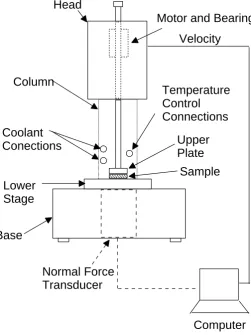
Description of a Stress-Controlled Shear Rheometer . . . 74
Parallel-Plate Geometry . . . 74
3.3.3 Dynamic Light Scattering . . . 78
3.3.4 Optical Microscopy and Particle Tracking . . . 79
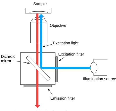
Fluorescence Microscopy . . . 79
Image Processing . . . 81
4.1 Introduction . . . 86
4.2 Materials and Methods . . . 89
4.2.1 Sample Preparation . . . 89
4.2.2 Atomic Force Microscopy . . . 89
4.2.3 Oscillatory Method . . . 90
4.2.4 Static Method . . . 96
4.3 Results and Discussion . . . 98
4.3.1 PVA Nanobers . . . 98
4.3.2 PVA Hydrogels . . . 105
4.4 Conclusion . . . 109
5 Rheology and Structure of Poly(vinyl alcohol)-Poly(ethylene glycol) Blends during Aging 114 5.1 Introduction . . . 114
5.2 Experiment . . . 117
5.2.1 Materials . . . 117
5.2.2 Measurements and Data Analysis . . . 117
5.3 Results . . . 120
5.3.1 Rheological Measurements . . . 120
5.3.2 Dynamic Light Scattering . . . 126
5.4 Discussion . . . 136
5.5 Conclusion . . . 141
6 Microrheology, Microstructure, and Aging of Physically Cross-Linked Poly(vinyl alcohol)/Poly(ethylene glycol) Blends 146 6.1 Introduction . . . 146
6.2 Experiment . . . 148
6.2.1 Sample Preparation . . . 148
6.2.2 Dynamic Light Scattering . . . 148
6.2.3 Video-Based Particle Tracking . . . 149
6.2.4 Microrheology . . . 151
6.3 Results . . . 153
6.3.1 Dynamic Light Scattering . . . 153
6.3.2 Video-Based Particle Tracking . . . 164
6.4 Discussion . . . 174
6.5 Conclusion . . . 180
7 Summary and Discussion 185 7.1 Summary . . . 185
7.1.1 The New Atomic Force Microscopy Technique for Measuring Viscoelas-ticity . . . 185
7.1.3 Microstructure and Microrheology of Poly(vinyl alcohol)/Poly(ethylene
glycol) . . . 187
7.2 Discussion . . . 188
7.2.1 Signicance of Work . . . 188
7.2.2 Future Work . . . 188
1.1 Schematic plot of viscosity as a function of shear rate for a polymer solution. 6 1.2 Schematic plot of the stress relaxation modulus of a polymer material as a
function of temperature. . . 7
1.3 Schematic plot of the shear modulus of materials as a function of frequency. 8 2.1 Schematic diagram showing a sphere in a viscous ow. . . 25
2.2 Schematic diagram showing scattering by two particles. The detector is far from the scattering particles. After [12]. . . 38
2.3 Schematic for dynamic light scattering for two particles. . . 43
2.4 Schematic for typical behavior of the intensity autocorrelation function. . . . 44
2.5 Contribution of a single subchain to the stress tensor. After [12]. . . 56
2.6 Illustration of the dependence of zero-shear viscosity η and equilibrium mod-ulus G on extent of percolation p for a cross-linking system. pc is the gel point. . . 62
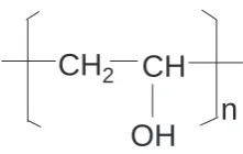
3.1 Molecular structure of poly(vinyl alcohol). . . 68
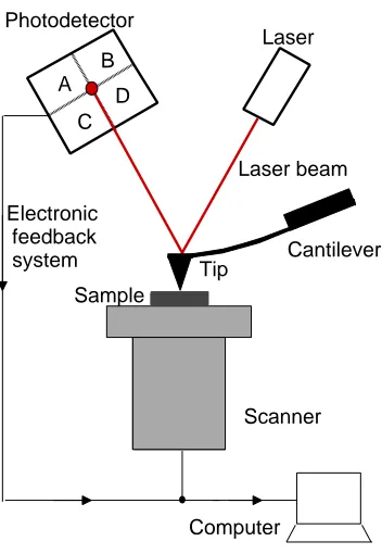
3.2 Schematic of an AFM. . . 71
3.3 Schematic of a force curve measured by the AFM when the tip approaches and retracts from the sample surface. . . 73
3.4 Schematic of the AR 1500ex rheometor. . . 75
3.5 Parallel plate geometry. . . 76
3.6 Schematic of the light scattering apparatus. . . 80
3.7 A schematic diagram of the light path of an inverted uorescence microscope. 81 4.1 Schematic showing the basic operation of the AFM in contact mode, with modications described in the text. . . 91
4.2 Illustration of the deformation of a ber clamped to supports a distance L apart while subject to a vertical force F applied at a distance x from one end of the ber. . . 93
4.3 Deformation a soft surface depressed by a rigid sphere of radius Rthat is glued under an AFM tip. . . 94
4.4 AFM images for a suspended ber: (a) height image; (b) oscillation amplitude image. . . 100
4.5 Oscillation amplitude z0 as a function of position along a suspended ber. . . 101
4.6 Young's modulus of a PVA ber as a function of frequency. . . 102
4.7 Relative slope as a function of distance along suspended bers. . . 104
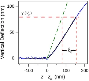
4.8 Force curve used to determine δ0 for the oscillatory method. . . 107
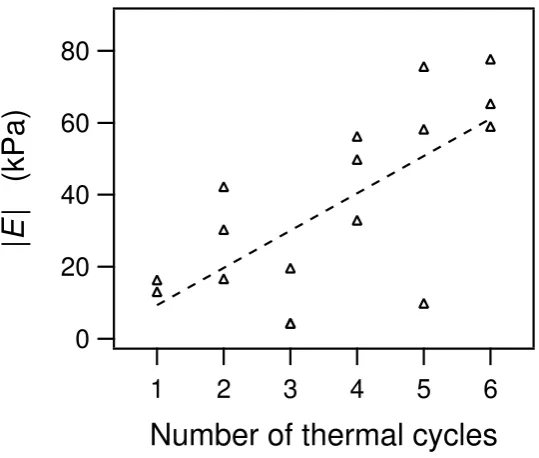
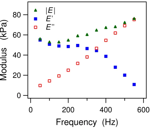
during preparation. . . 108 4.10 Complex modulus of a PVA hydrogel (four thermal cycles) as a function of
frequency. . . 109 4.11 Comparison of moduli determined by static force curve tting technique and
the oscillatory technique at 50 Hz. . . 110 5.1 Concentration dependence of the zero-shear-rate viscosity of PVA solutions. . 120 5.2 Viscosity as a function of shear rate determined from steady-state ow
mea-surements for a 10% PVA solution. . . 121 5.3 Viscosity of PVA/PEG blends with dierent concentrations of PEG as a
func-tion of shear rate. . . 122 5.4 Storage and loss moduli for the PVA solution and PVA/PEG blends during
aging. . . 124 5.5 G′ and G′′ at ω = 1 s−1 as a function of age for the pure PVA and the
PVA/PEG blends. . . 126 5.6 Logarithmic slope n1 of G′(ω) at low frequencies versus aging time and
mod-ulus ratio tanδ versus frequency for PVA/PEG blends. . . 127
5.7 Field autocorrelation function g(1)(τ) for 10% PVA solution at dierent
scat-tering angles. . . 128 5.8 Field autocorrelation function g(1)(τ) for PVA/PEG blends at a scattering
angle of 90◦ and at dierent ages. . . 130
5.9 Parameters obtained by tting the eld autocorrelation functions to KWW model in Eq. (5.2). . . 132 5.10 Distribution of relaxation times computed by the inverse Laplace transform
method for a 10% PVA solution and a 10% PVA/7% PEG blend at dierent aging times. . . 133 5.11 Intensity autocorrelation functions for PVA/PEG blends with concentrations
of PEG and aging time. . . 135 6.1 Mean square displacements of 110 nm microspheres measured from dynamic
light scattering experiments in water and PVA/PEG blends. . . 153 6.2 Microscopic viscosity ηm and local elasticity Ge of the PVA/PEG blends as a
function of PEG concentration. . . 154 6.3 ⟨ ∆r2(τ)⟩ a for microspheres with dierent sizes measured from dynamic light
scattering experiments in a 10% PVA solution and a 10% PVA/7% PEG blend. 157 6.4 Mean square displacements of 110 nm microspheres measured from dynamic
light scattering experiments in a 10% PVA/7% PEG blend at dierent aging times. . . 158 6.5 (a) Mean square displacement and the logarithmic slopes at short,
interme-diate, and long lag times as a function of aging time for tracer particles in a 10% PVA/7% PEG blend. . . 159
6.7 Crossover frequencies ω1 and ω2, the minimum value of the G′′ G′′min, and the
micro-elastic modulus G′e as a function of PEG concentration. . . 161
6.8 Microscopic viscous and elastic modulus for a 10% PVA/7% PEG blend. . . 163 6.9 Mean square displacements of 110 nm microspheres measured from video-based
particle tracking experiments in freshly prepared blends. . . 165 6.10 Mean square displacements, distribution of individual particle displacements
at a lag time of 1 s and that averaged over all particles, and individual particle trajectories in a 10% PVA solution. . . 167 6.11 Mean square displacements, distribution of individual particle displacements
at a lag time of 1 s and that averaged over all particles, and individual particle trajectories in a 10% PVA/7% PEG blend. . . 168 6.12 Elasticity as a function of aging time. . . 171 6.13 Viscous and elastic moduli calculated from video particle tracking data for
particles in a 10% PVA sample. . . 172 6.14 Viscous and elastic moduli calculated from video particle tracking data for
particles in a 10% PVA/7% PEG blend. . . 173
5.1 Composition of the polymer blends. . . 117
Chapter 1
Introduction
1.1 Viscoelastic Properties of Soft Materials
Complex uids such as polymer solutions, gels, emulsions, and colloidal suspensions play a ubiquitous role in everyday life. They encompass biomaterials, foods, personal care products, and a range of industrial products [1]. Complex uids were rst referred to as soft materials by P.-G. de Gennes in his Nobel lecture [2]. These materials can both store and dissipate energy when deformed by an external force. A simple solid stores energy in response to applied stress and behaves as a Hookean spring, while a simple liquid dissipates energy through viscous Newtonian ow [1]. Most soft materials exhibit both solid-like and liquid-like responses, which generally depend on the time scale or frequency at which the sample is probed. These materials are thus viscoelastic [3].
Soft materials exhibit complicated ow properties which distinguish them from other ma-terials [1]. Here, we use ow to refer to a smooth, irreversible deformation on an accessible time scale. Solids will not ow, but rather deform elastically under modest stresses and de-form irreversibly or fracture under larger stress. Liquids will always ow viscously no matter how small the applied stress. The ow behavior of a complex uid is not this simple. For example, honey is a uid that has high viscosity, but is nonetheless Newtonian. If one dis-turbs the surface of honey in a jar, it will slowly return to its original, level shape under the force of gravity. In contrast, mayonnaise behaves quite dierently. A perturbed mayonnaise surface remains perturbed minutes or even a year after it has been disturbed. Materials like mayonnaise are solid-like under moderate stress and will ow only when the applied stress exceeds a threshold value called the yield stress. The existence of a yield stress means that a non-zero stress is required to cause ow, and the stress must remain above the yield stress for sustained ow.
Examples of complex uids also include biomaterials such as blood and personal care products such as shampoo and toothpaste [1]. The ow behavior of blood is shear-rate-dependent due to the presence of the red blood cells. At modest shear rates, the ow and orientation of the red blood cells are similar to those of rigid disks, while at higher shear rates they deform to resemble uid droplets. The viscoelastic properties of blood are important to the human body as they determine the pumping load on the heart. The behavior of personal care products can be controlled by varying their compositions. Shampoos are designed to ow readily, but not too quickly, from the tube or bottle into one's hand. Toothpaste must ow out of the tube only when squeezed, and stop owing and hold its shape immediately after it has been applied to the brush.
expense of processing, and to some extent, the properties of the nal products [1].
Overall, soft materials have mechanical behavior intermediate between simple liquids and solids. Most are solids at short times and liquids at long times. The characteristic time required for them to change from solid to liquid varies from fractions of a second to days, or even years, depending on the uid. Some complex uids change from solid-like to liquid-like when subjected to a modest deformation, such as particulate and polymeric gels [1]. Others, such as electrorheological and magnetorheological suspensions, will change from liquid-like to solid-like when an electric or magnetic eld is applied [1].
1.2 Rheology
Rheology is the study of the viscoelasticity of materials. It can be dened as the measurement and study of the relationship between the deformation (strain) of a material and the stress [1, 4]. This eld involves inquiry into the ow behavior of complex uids such as polymers, foods, biological systems, and other compounds. The relation between stress and deformation for these materials diers from Newton's law of viscosity, which describes the shear behavior of simple liquids:
σ =ηγ,˙ (1.1)
where σ is the stress, η is a constant of proportionality called the Newtonian viscosity, γ is
the strain, or relative change in length, and γ˙ = dγ/dt is the rate of strain. Newton's law
thus states that the stress is proportional to γ˙.
The relationship between stress and deformation of complex materials also diers from Hooke's law of elasticity, the relationship that holds for metals and other elastic materials,
σ=Gγ, (1.2)
of the solid material [1].
Instead, the relationship between the stress and strain of a complex uid is intermediate between these two limiting cases. A major goal of rheology is to determine the equations, referred to as constitutive equations, that correctly describe the behavior of particular ma-terials. These are often based on combinations and generalizations of the above equations.
Satisfactory constitutive equations can be determined through experiments. For example, one can apply a shear deformation and measure the resultant stress as a function of the shear rate. The functions of the kinematic parameters that characterize the rheological behavior of uids are called rheological material functions. One commonly used material function relates the constant strain rateγ˙ in a steady ow experiment to the shear stress σ. For a Newtonian
uid, the stress σ is constant and the material function is
η = σ ˙
γ. (1.3)
η is therefore also constant and independent of γ˙. For non-Newtonian uids, on the other
hand, viscosity will be a function of shear rate, i.e., η = η( ˙γ). If η decreases with γ˙, the
material is called shear thinning. Ifηincreases withγ˙, in contrast, it is called shear thickening.
Two other material functions widely used to characterize the viscoelastic properties of soft materials describe their response to small amplitude oscillatory shear (SAOS). They are dened based on an imposed sinusoidal shear strain
γ =γ0sin(ωt), (1.4)
and the resulting shear stress
σ = σ0sin(ωt+δ)
where δ is the phase dierence between the applied strain and the stress response. From
Eqs. (1.4) and (1.5) one can derive expressions for the storage modulus G′(ω) and the loss
modulusG′′(ω):
G′(ω) = σ0
γ0
cosδ, (1.6)
and
G′′(ω) = σ0
γ0
sinδ. (1.7)
G′ is thus the amplitude of the component of the oscillatory stress that is in phase with the
applied strain divided by the amplitude of the strain oscillation. G′′ is dened analogously
as the amplitude of the stress component that is out of phase with the strain, divided by the amplitude of the strain. For a Newtonian uid in SAOS, the response is completely out of phase with the strain, so G′ = 0 and η = σ/γ˙ =G′′/ω. For an elastic solid that follows
Hooke's law, the shear-stress response in SAOS is completely in phase with the strain: G′ =G
and G′′= 0.
Transient rheological measurements are also common. They include stress relaxation mea-surements, in which a constant strain γ is applied for a certain time, then released, allowing
a time-dependent relaxation modulus G(t) to be measured as G(t) = σ(t)/γ, where σ(t) is
the time-dependent stress. In a creep test, a constant stress is applied to the material and the resultant time-dependent strain is measured.
1.3 Rheological Behavior of Polymer Materials
γ
η
η
0η
8Newtonian plateau
Shear thinning
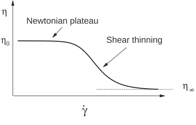
Figure 1.1: Schematic plot of viscosity as a function of shear rate for a polymer solution.
of strain rate γ˙ for a typical polymer solution. The viscosity falls from the zero-shear value
η0 at lowγ˙ to a lower valueη∞in the limit of innite shear rate. Depending on the material,
the dierence between η0 and η∞ can be several orders of magnitude. The decrease of η is
due to disentanglement and alignment of the polymer molecules under shear. The inverse of the shear rate at which the viscosity starts to decrease is determined by the time needed for the entangled polymers to relax.
The viscoelastic properties of polymeric materials are dependent on temperature and time. Fig. 1.2 shows an idealized plot of the relaxation modulus G as a function of temperature
10
9
8
7
6
5
4
3
Log G (Pa)
Temperature
Glassy
Transition
Rubbery
Crosslinked
Linear
Flow
Figure 1.2: Schematic plot of the stress relaxation modulus of a polymer material as a function of temperature.
diusion of the polymer segments becomes possible, and segments are free to jump from one conguration to another. At even higher temperatures, the modulus reaches a second plateau. This rubbery plateau is due to the presence of strong local interactions between neighboring chains, which restrict the long-range cooperative diusion of complete molecules. In a linear polymer, these interactions are known as entanglements. In the case of a cross-linked material, they consist of chemical or physical bonds. In a linear polymer, as the temperature is further increased, the entanglements relax and the molecules become able to ow so the modulus again decreases [6]. In a chemically cross-linked system, however, the crosslinks will remain intact, and the modulus remains constant until the temperature is high enough for chemical degradation.
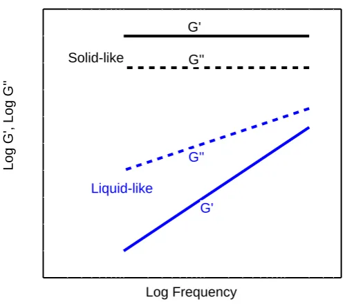
Log G', Log G''
Log Frequency G' G'' G'
G'' Solid-like
Liquid-like
Figure 1.3: Schematic plot of the shear modulus of materials as a function of frequency.
connected to form a gel network. The storage modulus G′ and loss modulus G′′ of liquid-like
and solid-like materials behave very dierently as a function of frequency ω, as shown in Fig.
1.3, and therefore they can be used to characterize the gelation of a system. For liquid-like materials,G′′is much higher than G′ and, at frequencies smaller than the shortest relaxation
rate in the system, and one expects G′′ ∝ ω and G′ ∝ ω2 [1]. For solid-like materials, in
contrast,G′ is much higher than G′′ and both G′ and G′′ are nearly frequency-independent,
due to the existence of structures that can not relax over the time scales being probed [1]. At the gel transition, G′ and G′′ both show a power-law dependence on frequency, with G′ ∼ G′′ ∝ ων, where ν is a power-law index [5]. This will be discussed in more detail in
1.4 Microrheology
Soft materials such as polymer solutions and gels are typically structured on the microscopic scale. The techniques of microrheology have been developed to probe viscoelastic properties on such scales [3, 7]. This relatively new set of techniques can be used to investigate how the viscoelasticity of materials changes with length scale. From this, information about the materials' microstructure can be obtained.
Microrheology involves using micron-sized tracer particles suspended in the material to locally measure the rheology of complex materials. This typically involves extracting the local viscous and elastic moduli from measurements of the motion of the tracers. There are two main classes of microrheological methods, distinguished by how the particle motion is driven. One class involves the active manipulation of probes by external elds and is called active microrheology. The other involves measuring the motion of the particles due to thermal uctuations and is referred to as passive microrheology. In either case, the interpretation of the measurements depends on the size of the probe particle relative to the structural length scales in the material. If the embedded particles are larger than any structural scale, the particle motion measures the macroscopic properties of the material. If they are smaller than the structural size, local rheological properties can be measured.
1.4.1 Active Microrheology
Magnetic tweezers can be used to manipulate magnetic particles suspended in a material for active microrheology [8]. The motion of these particles is measured and related to the local rheology of the material. This method has been used to measure the microrheology of a number of interesting materials, such as networks of lamentous actin [9, 10], living cells [11] and double-helical structured DNA [12].
fo-cused beam of light captures and manipulates small dielectric particles. The two main op-tical forces exerted on an illuminated particle are the scattering forces, which act along the direction of beam propagation, and the gradient force, which arises from induced dipole inter-actions with the electric eld gradient. The resultant force tends to pull the particle towards the focus. Moving the focused laser beam forces the particle to move, applying a local stress to the surrounding material and allowing the local rheological response to be probed [13]. Probe particles can be driven in either oscillatory or translational motion so both frequency-dependent and steady state properties can be measured [14]. The forces applied by optical tweezers are very local and typically limited to the pN range. Optical tweezers have been used to measure the microrheology of complex materials such as membranes with cytoskeletal proteins [15], solutions of DNA [16] and colloidal suspensions [17, 18].
A third active microrheological technique involves using an atomic force microscope (AFM). In addition to imaging surface structure and topology, AFM techniques are sensitive to the force required to deform a surface and have been used to measure the local elasticity and viscoelasticity of soft materials. An AFM measures forces by monitoring the deection of a tip connected to a cantilever spring brought into contact with the surface. The force exerted by the cantilever can be calculated using Hooke's law. Mahay et al. probed surfaces using an AFM cantilever with a polystyrene bead glued underneath of the tip. By oscillating the cantilever when approaching the surface of a polyacrylamide gel, they successfully measured the viscoelastic response of the sample surface [19]. AFM techniques have been used to study soft materials such as gels [19], blood platelets [20] and cells [21, 22].
1.4.2 Passive Microrheology
method is to image the positions of uorescent probe particles using video microscopy. The ensemble-averaged mean squared displacement (MSD) of the particles can be used to calcu-late the frequency-dependent viscous and elastic moduli of the materials using a generalized Stokes-Einstein relation [23, 24], as will be discussed in detail in the next chapter. Depending on the size of the probe particles relative to the structure in the uid, the viscoelastic prop-erties determined in this way are a measure of either the local or the bulk propprop-erties of the material, as mentioned above. In two-particle microrheology, the cross-correlation function of the particle displacements is calculated as a function of particle separation [25, 26]. This can be used to infer information about the material structure and properties on dierent length scales. This provides a way to probe the bulk rheology of a heterogeneous sample using microrheology. The drawback of this technique is that a large amount of data is need-ed to obtain statistically meaningful results. Although particle tracking microrheology is restricted to relatively low frequencies, it is a fairly simple technique to implement. It has been applied to various materials, such as solutions of DNA [27], actin laments [28, 29], Carbopol gels [30, 31], cross-linked polyacrylamide networks [32], laponite clay suspensions [33] and polymer microgels [36].
Dynamic light scattering can also be used for microrheological measurements. An incoming laser beam illuminates a sample in which probe particles are suspended, and is scattered by the probe particles into a detector at a scattering angle θ. As the particles diuse in the
sample, the intensity of scattered light that reaches the detector uctuates in time. The autocorrelation function of the time-dependent intensity is calculated. With the assumption that the scattering is a Gaussian process and that the photons are scattered only once by the particles, the eld correlation function can be calculated from the intensity correlation function [35], allowing the ensemble-averaged mean squared displacement of the particles to be determined as a function of time. As above, the mean squared displacement can be used to calculate the micron-scale rheological properties of the material [30, 36].
mean squared displacement of the probe particles [35, 37]. Although the experimental set-up is similar to that of the single-scattering experiment, all angle-dependent information is lost as the photons are scattered through all possible angles. Diusing wave spectroscopy can be used for rheological measurements at frequencies up to 105 Hz. The microrheology of exible
and semi-exible polymer solutions has been studied using this technique [28, 38, 39].
1.5 Summary of Present Work
1.5.1 Overview
suggestions for future work are given in Chapter 7.
1.5.2 Frequency-Dependent Viscoelasticity Measurements by Atomic Force Mi-croscopy
The atomic force microscope (AFM) has been widely used to study the structure of soft and biological materials with sub-nanometer resolution. AFM is also used to measure the local elasticity and viscoelasticity of soft samples. The advantage of AFM measurements is that topographic images can be obtained simultaneously with the mechanical response, allowing elasticity to be correlated with local structure. One common technique, referred to as force volume imaging, involves indenting the sample by translating it through a vertical ramp at positions over a grid of sample positions [53]. The discrepancy between the known vertical displacement and resulting cantilever deection can be used to infer the elastic properties of the sample. The eects of non-vertical motion due to sliding of the inclined cantilever along the sample surface (e.g., shear deformation and frictional eects) as well as surface adhesion can complicate the analysis, however. In addition, force-volume imaging does not provide information about the viscous response. AFM measurements using intermittent contact mode or force modulation mode, both of which image surfaces with a cantilever oscillating at a small amplitude with a xed frequency, can reveal contrast in the viscoelastic properties of the sample, but their nonlinear behavior complicates the analysis [54, 55].
1.5.3 Viscoelastic Properties and Structural Evolution of Physically Cross-Linked Poly(vinyl alcohol)/Poly(ethylene glycol) Blends during Aging
As PVA molecules have a large number of hydroxyl groups, they aggregate easily in concen-trated solutions due to hydrogen bonding. The polymer aggregates form a network structure leading to gelation [56, 60, 61]. PVA has an upper critical solution temperature, and phase separates when quenched into the unstable region of the phase diagram. Consequently, gela-tion can take place in combinagela-tion with microphase separagela-tion [62, 63, 64, 65]. Because of this, the mechanism of gelation in physical PVA gels is still not well understood. We are also interested in studying the dependence of the gel transition on length scale. Although Matsunaga et al. found good agreement between the microscopic and macroscopic gel points of gelatin hydrogels [66], Oppong et al. observed that gelation of Laponite clay suspensions occurred earlier on the macroscopic scale than on the microscopic scale [33]. By studying gelation in PVA blends, we will explore this phenomenon.
We study the aging of physical PVA gels made by the theta-gel method [67, 68], in which PEG is added to the PVA solution as a gelling agent. The blends undergo gelation over a period of up to two months. We measure the rheological behavior using conventional rheometry. We also use dynamic light scattering to investigate the microstructural evolution as a function of PEG concentration and aging time, and determine the microscopic gel points of the PVA gels. We compare the gelation thresholds measured by the two techniques. This work will be presented in Chapter 5.
1.5.4 Microrheology, Microstructure, and Aging of Physically Cross-Linked Poly(vinyl alcohol)/Poly(ethylene glycol) Blends
materials as a function of PEG concentration and aging time.
BIBLIOGRAPHY
[1] R. G. Larson, The Structure and Rheology of Complex Fluids (Oxford University Press, New York, 1999).
[2] P. G. de Gennes, Rev. Mod. Phys. 64, 645 (1992).
[3] T. M. Squires and T. G. Mason, Annu. Rev. Fluid Mech. 42, 413(2010).
[4] F. A. Morrison, Understanding Rheology (Oxford University Press, New York, 2001). [5] M. Rubinstein and R. H. Colby, Polymer Physics (Oxford University Press, New York,
2003).
[6] M. T. Shaw and W. J. MacKnight, Introduction to Polymer Viscoelasticity (Wiley, New Jersey, 2005).
[7] T. A. Waigh, Rep. Prog. Phys. 68, 685 (2005).
[8] B. Chu and J. Wang, Rev. Sci. Instrum. 63, 2315 (1992).
[9] F. Ziemann, J. Radler, and E. Sackmann, Biophys. J. 66, 2210 (1994).
[10] F. Amblard, A. C. Maggs, B. Yurke, A. N. Pargellis, and S. Leibler, Phys. Rev. Lett. 77, 4470 (1996).
[11] B. Fabry, G. N. Maksym, J. P. Butler, M. Glogauer, D. Navajas, and J. J. Fredberg, Phys. Rev. Lett. 87, 1481021 (2001).
[13] A. Ashkin, Biophys. J. 61, 569 (1992).
[14] L. A. Hough and H. D. OuYang, J. Nanopart. Res. 1, 495 (1999).
[15] E. Helfer, S. Harlepp, L. Bourdieu, J. Robert, F. C. MacKintosh, and D. Chatenay, Phys. Rev. E 63, 021904 (2001).
[16] T. T. Perkins, D. E. Smith, R. G. Larson, and S. S. Chu, Science 268, 83 (1995). [17] P. Habdas, D. Schaar, C. A. Levitt, and E. R. Weeks, Europhys. Lett. 67, 477 (2004). [18] A. Meyer, A. Marshall, B. G. Bush, and E. M. Furst, J. Rheol. 50, 77 (2006).
[19] R. E. Mahay, C. K. Shih, F. C. MacKintosh, and J. Kas, Phys. Rev. Lett. 85, 880 (2000).
[20] M. Radmacher, M. Fritz, C. M. Kasher, Biophys. J. 70, 556 (1996).
[21] C. Rotsch, F. Braet, E. Wisse, and M. Radmacher, Cell Biol. Int. 21, 685 (1997). [22] C. Rotsch and M. Radmacher, Biophys. J. 78, 520 (2000).
[23] T. G. Mason and D. A. Weitz, Phys. Rev. Lett. 74, 1250 (1995). [24] T. G. Mason, Rheol. Acta 39, 371 (2000).
[25] T. C. Lubensky and A. J. Levine, Phys. Rev. Lett. 85, 1774 (2000).
[26] J. C. Crocker, M. T. Valentine, E. R. Weeks, T. Gisler, P. D. Kaplan, A. G. Yodh, and D. A. Weitz, Phys. Rev. Lett. 85, 888 (2000).
[27] T. G. Mason, A. Dhople, and D. Wirtz. Mater. Res. Soc. Symp. Proc. 463, 153 (1997). [28] J. Y. Xu, V. Viasno, and D. Wirtz, Rheol. Acta 37, 387 (1998).
[30] F. K. Oppong, L. Rubatat, B. J. Frisken, A. E. Bailey, and J. R. de Bruyn, Phys. Rev. E 73, 041405 (2006).
[31] F. K. Oppong and J. R. de Bruyn, J. NonNewtonian Fluid Mech. 142, 104 (2007). [32] B. R. Dasgupta and D. A. Weitz, Phys. Rev. E 71, 021504 (2005).
[33] F. K. Oppong, P. Coussot, and J. R. de Bruyn, Phys. Rev. E 78, 021405 (2008). [34] D. van den Ende, E. H. Purnomo, M. H. G. Duits, W. Richtering, and F. Mugele, Phys.
Rev. E 81, 011404 (2010).
[35] W. Brown, Dynamic Light Scattering: The Method and Some Applications (Oxford Univ. Press, New York, 1993).
[36] T. G. Mason, H. Gang, and D. A. Weitz, J. Molec. Struct. 383, 81 (1996). [37] T. G. Mason, H. Gang, and D. A. Weitz, J. Opt. Soc. Am. A 14, 139 (1997).
[38] B. R. Dasgupta, S.-Y. Tee, J. C. Crocker, B. J. Frisken, and D. A. Weitz, Phys. Rev. E 65, 051505 (2002).
[39] A. Palmer, T. G. Mason, J. Xu, S. C. Kuo, and D. Wirtz, Biophys. J. 76, 1063 (1999). [40] S. W. Lovesey and E. W. J. Mitchell, Polymer and Neutron Scattering (Oxford
Univer-sity Press, New York, 1994).
[41] M. Shibayama, Polym. J. 43, 18 (2011).
[42] S. D. Hudson, J. L. Hutter, M.-P. Nieh, J. Pencer, L. E. Millon, and W. Wan, J. Chem. Phys. 130, 034903 (2009).
[43] O. Urakawa, H. Ikuta, S. Nobukawa, T. Shikata, J. Polym. Sci. B: Polym. Phys. 46, 2556 (2008).
[45] M. Shibayama, S. Miyazaki, H. Endo, T. Karino, and K. Haraguchi, Macromol. Symp. 256, 131 (2007).
[46] T. Nishida, H. Endo, N. Osaka, H. J. Li, K. Haraguchi, and M. Shibayama, Phys. Rev. E 80, 030801 (2009).
[47] T. Matsunaga, T. Sakai, Y. Akagi, U. Chung, and M. Shibayama, Macromolecules 42, 1344 (2009).
[48] H. Endo, D. Schwahn, and J. Colfen, J. Chem. Phys. 120, 9410 (2004). [49] M. V. Avdeev and V. L. Aksenov, Physics-Uspekhi 53, 971 (2010). [50] W.T. Heller, Acta. Cryst. 66, 1213 (2010).
[51] M. Takeda, T. Matsunaga, T. Nishida, H. Endo, T. Takahashi, and M. Shibayama, Macromolecules 43, 7793 (2010).
[52] T. Matsunaga, H. Endo, M. Takeda, M. Shibayama, Macromolecules 43, 5075 (2010). [53] G. Guhados, W. K. Wan, and J. L. Hutter, Langmuir 21, 6642 (2005).
[54] L. Nony, R. Boisgard, and J. P. Aime, J. Chem. Phys. 111, 1615 (1999).
[55] S. L. Lee, S. W. Howell, A. Raman, and R. Reifenberger, Phys. Rev. B 66, 115409 (2002).
[56] C. M. Hassan, and N. A. Peppas, Adv. Polym. Sci. 153, 37 (2000).
[57] M. Qi, Y. Gu, N. Sakata, D. Kim, Y. Shirouzu, Ch. Yamamoto, A. Hiura, S. Sumi, and K. Inoue, Biomaterials 25, 5885 (2004).
[58] M. Kobayashi, Y.-S. Chang, and M. Oka, Biomaterials 26, 3243 (2005).
[60] S. D. Hudson, J. L. Hutter, M.-P. Nieh, J. Pencer, L. E. Millon, and W. Wan, J. Chem. Phys. 130, 034903 (2009).
[61] T. Narita, A. Knaebel, J. P. Munch, and S. J. Candau, Macromolecules 34, 8224 (2001). [62] T. Kanaya, M. Ohkura, H. Takeshita, K. Kaji, M. Furusaka, H. Yamaoka, and G. D.
Wignall, Macromolecules 28, 3168 (1995).
[63] H. Takeshita, T. Kanaya, K. Nishida, and K. Kaji, Macromolecules 32, 7815 (1999). [64] H. Takeshita, T. Kanaya, K. Nishida, and K. Kaji, Macromolecules 34, 7894 (2001). [65] N. Takahashi, T. Kanaya, K. Nishida, and K. Kaji, Macromolecules 40, 8750 (2007). [66] T. Matsunaga and M. Shibayama, Phys. Rev. E 76, 030401(R) (2007).
[67] E. Oral, H. Bodugoz-Senturk, C. Macias, and O. K. Muratoglu, Nucl. Instrum. Meth. B 265, 92 (2007).
Chapter 2
Theory
2.1 Introduction
In this Chapter, we review the basic theory behind the experimental techniques used in this thesis. The Chapter is divided into four Sections; a summary of each is given below.
We introduce the theory of the motion of suspended particles in simple and complex uids in Section 2.2. We discuss Brownian motion and its characteristics, as well as Stokes' law and the Langevin equation. Stokes' law describes the frictional force exerted on spherical objects in a viscous uid. The Langevin equation is the equation of motion for particles moving in a viscous uid. We derive an expression for the mean squared displacement of the particles in terms of the diusion coecient from both the Langevin equation and the diusion equation. Then we derive the Stokes-Einstein relation by combining Stokes' law and diusion theory. We then introduce a generalized Langevin equation which includes a memory function as the equation of motion for particles moving in a viscoelastic uid. The generalized Stokes-Einstein relation is used to derive expressions for the viscoelastic moduli of the uid. The material presented in this section follows the work in Refs. [1, 2, 3, 4].
scattered electromagnetic eld far from the scattering centers. We then introduce several simplifying assumptions to describe light scattering by a dilute suspension of discrete spheri-cal particles. We introduce the dynamic light scattering technique used to study the diusion of the scattering particles, and dene the intensity and electric eld correlation functions. The discussion in this section is primarily based on Refs. [6, 7, 8, 9].
In Section 2.4, we discuss the basic theory of the rheological behavior of polymers. We introduce the concept of linear viscoelasticity for soft materials. We start from the Mawell model and derive the generalized linear viscoelastic model, which is used to calculate the viscous and elastic moduli characterizing the response to a sinusoidally varying deformation [12, 13, 14].
Finally, in Section 2.5, we introduce the theoretical models that describe the dynamics of polymer molecules in both the dilute and concentrated regimes. To model the dilute regime, we discuss the Rouse model, while for the concentrated limit, we review the reptation or tube model. We discuss these models in the context of their predictions for the stress relaxation modulus and the viscous and elastic moduli. We also introduce the concept of gelation and discuss the rheological behavior of uids near a gel point. The discussion in this section is based on Refs. [12, 15, 16].
2.2 The Motion of Particles in Simple and Complex Fluids
2.2.1 Brownian Motion
nature of matter [18]. Einstein was able to determine the mean squared displacement (MSD) of a Brownian particle in terms of Avogadro's number. In 1926, Jean Perrin won the Nobel Prize for determining Avogadro's number using this method [19].
Formally, Brownian motion is a stochastic process and can be described by a random walk model. Typically, each step in the walk is of constant length but the direction of the walk from one point to the next is completely random. We let l be the step length of a particle
undergoing a random walk. Let the origin be at r0 = 0. After N steps, the particle will be
at the point rN. After N+1 steps, the position of the particle will be
rN+1 =rN +ln, (2.1)
where n is the unit vector in the direction of the (N+ 1)th step, that is, the direction of the
step taken by the particle located at the point rN.
Because the direction of each step is random, we have ⟨ n⟩ = 0, where the angular brackets
denote as average over an ensemble of particles. As a result, if we take the average of both sides of Eq. (2.1), we have
⟨ rN+1⟩ =⟨ rN⟩ . (2.2)
Eq. (2.2) indicates that for all N
⟨ rN⟩ =⟨ rN−1⟩ =...= 0, (2.3)
that is,
⟨ rN⟩ = 0 (2.4)
for all N.
not zero, however. Einstein was able to show that
⟨ r2⟩
= 2Dt, (2.5)
for one dimensional motion [1, 4], where D is the diusion coecient. We will derive Eq.
(2.5) through the Langevin equation in Section 2.2.3, and through the diusion equation in Section 2.2.4.
The central limit theorem expresses the fact that any sum of many statistically independent random variables is normally distributed [1, 2, 4]. Hence such a random variable has a prob-ability distribution function that can be described by the normal or Gaussian distribution. This represents the probability of occurrence of each value of the random variable x and is
given by
f(x) = 1
σ√ 2πe
−(x−µ)2/2σ2
, (2.6)
whereµ is the mean and σ is the standard deviation of the distribution.
The displacement of a particle performing Brownian motion is the result of many random forces and so, by virtue of the central limit theorem, can be described by the Gaussian distribution function.
2.2.2 Stokes' Law
Stokes' law was derived by George Gabriel Stokes in 1851 to describe the friction or drag force exerted on spherical objects moving in a viscous uid at very low speed [3]. We can derive this law from the equations of uid dynamics. Consider a stationary sphere with radiusa in a viscous ow as shown in Fig. 2.1. The ow eld v(r, t)can be described by the
Navier-Stokes equation
(v· ∇ )v=−1
ρ∇ p+η∇ 2v
v
a θ
Figure 2.1: Schematic diagram showing a sphere in a viscous ow.
where ρ is the density and η the viscosity of the uid, p is the pressure, and g is the
accel-eration due to gravity. We consider the case that the Reynolds number R, which is dened
as
R= V a
η , (2.8)
is very small, i.e., R ≪ 1. Here, V is the ow speed far from the sphere. The Reynolds
number is an indication of the relative magnitudes of the inertial term, (v· ∇ )v, to the
viscous term, η∇ 2v, in Eq. (2.7). For R ≪ 1, the inertial term is much smaller than the
viscous term and Eq. (2.7) simplies to
0 =− 1
∇ p+µ∇ 2v, (2.9)
in the absence of body forces. We also have
∇ · v= 0 (2.10)
for an incompressible uid. To solve Eq. (2.9), we work in spherical polar coordinates and introduce the scalar Stokes stream function Ψ(r, θ), such that
vr = 1
r2sinθ ∂Ψ
∂θ , (2.11)
and
vθ =− 1
rsinθ ∂Ψ
The boundary conditions onΨare ∂∂rΨ = 1r∂∂θΨ = 0on r=a, andvr =V cosθandvθ =V sinθ
asr→ ∞ . We try a solution of the form
Ψ =f(r) sin2θ. (2.13)
Upon substitution into Eqs. (2.9) and (2.10), we nd
(
d2 dr2 −
2
r2
)2
f = 0. (2.14)
This equation has a solution for f of the form rα provided that
[(α− 2)(α− 3)− 2][α(α− 1)− 2] = 0, (2.15)
from whichα=−1, 1, 2 or4. Thus
f(r) = A
r +Br+Cr
2+Dr4, (2.16)
whereA, B, C and D are arbitrary constants. Applying the boundary conditions, we have
Ψ = 1
4V(2r 2+ a3
r − 3ar) sin
2θ. (2.17)
Having found Ψ, we can calculate the pressure using Eq. (2.9)
p=p∞− 3
2
µV a
r2 cosθ. (2.18)
The radial and tangential stress components on the surface of the sphere are given by the constitutive equation for incompressible uid [3] and we have
tr=−p∞+
3 2
µV
a cosθ, and tθ =−
3 2
µV
By symmetry, we expect the net force on the sphere to be in the direction of the ow, and the appropriate component of the stress vector is thus t =trcosθ− tθsinθ. The drag force
on the sphere is the stress integrated over the surface of the sphere,
Fdrag =
∫ 2π
0
∫ π
0
ta2sinθdθdϕ= 6πµV a. (2.20)
Eq. (2.20) is the Stokes relation. It says that a spherical particle moving in a viscous uid experiences a drag force that is proportional to its speed relative to the uid.
2.2.3 Langevin Equation and the Fluctuation-Dissipation Theorem
The Langevin equation is an equation of motion for particles moving in a uid [2, 4]. It can be used in combination with the central limit theorem to quantitatively describe Brownian motion. In this section, we derive the Langevin equation for a Brownian particle moving in a simple uid and introduce the uctuation-dissipation theorem.
We consider a suspended microsphere undergoing Brownian motion in a liquid. Since its direction of motion changes, the sphere accelerates. The acceleration is due to the net force exerted on it. The forces on the microsphere include the downward force due to gravity, the upward buoyancy force, a random uctuating force F(t), and the drag force f. Gravity is
balanced by buoyancy as the sphere is suspended in the uid. The random uctuating force is the sum of the forces exerted on the sphere by all the molecules in the liquid that it is in contact with. The molecules move randomly and hence the net force they exert on the sphere is also random. As it moves through the liquid, the miscrosphere experiences a Stokes drag that is proportional to the velocity of the sphere, f = −αv, where v is the velocity
of the particle with respect to the liquid and α is the drag force coecient. For a particle
performing Brownian motion, Newton's second law gives
mdv(t)
wherem is its mass andt is time. Consider two time scales in the Brownian motion problem.
One is that over which correlations in the motion of the liquid molecules persist and the second is the time scale over which the suspended particle experiences a signicant change in its velocity. Since the motion of the liquid molecules is much faster than that of the suspended particle, the second time scale is much longer than the rst. If we consider two times t and t′ separated by an interval long enough that the motion of the liquid molecules
at the two times is uncorrelated, then the forces F(t) and F(t′), will also be uncorrelated, so
⟨ F(t)·F(t′)⟩ =βδ(t− t′), (2.22)
where β is a constant and δ is the Dirac delta function. Since F(t) is independent of the
frictional drag −αv, we also have
⟨ v(0)·F(t)⟩ = 0 (2.23)
fort >0. Using these results, the general solution of Eq. (2.21) is given by
v(t) =v(0) exp
( − α mt ) + ∫ t 0
dt′F(t
′)
m exp
(
− α
m(t−t
′)). (2.24)
Eqs. (2.21) (2.24) constitute the Langevin model for the motion of a Brownian particle.
From the equipartition theorem, the mean square velocity of a particle in thermal equilib-rium is
⟨ v2(t)⟩ = 3kT
m , (2.25)
where k is the Boltzmann constant and T is temperature. Using Eq. (2.24) and taking the
ensemble average, we have
⟨ v2(t)⟩ = ⟨ v2(0)⟩ exp(−2α
mt) +
2
m
∫ t
0
dt′⟨ v(0)·F(t)⟩ exp(−2α
m(t− t
′)) + ∫ t 0 dt′ ∫ t 0
dt′′⟨ F(t
′)·F(t′′)
m2 ⟩ exp(− α
m(2t− t
All ⟨ v2⟩ terms in Eq. (2.26) can be replaced by 3kT /m, and the rst integral on the right
hand side vanishes according to Eq. (2.23). We use Eq. (2.22) to remove the delta function by performing one of the integrals of the third term on the righthand side of Eq. (2.26). Eq. (2.26) then becomes
3kT m
(
1− exp(−2α
mt)
)
= β
m2
∫ t
0
dt′exp
(
exp(−2α
m(t− t
′)). (2.27)
After integration and simplication of Eq. (2.27), we get
β = 6αkT, (2.28)
so Eq. (2.22) becomes
⟨ F(t)·F(t′)⟩ = 6αkT δ(t− t′). (2.29)
Eq. (2.29) is referred to as the uctuation-dissipation theorem [5]. This theorem relates the uctuations in a system at thermal equilibrium to the response of the system. The random force F that causes the erratic motion of a particle has the same origin as the frictional force −αv which causes the energy dissipation. The theorem shows that the mean-square
value of a uctuating force is related to the corresponding friction factor. If there was no uctuating force F acting on the diusing particles, then the velocity v and the kinetic energy of the particles would decrease exponentially and eventually vanish. The random force acts to restore the kinetic energy of the diusing particles so that it remains constant on average [5].
2.2.4 Mean Squared Displacement from the Langevin Equation
Eq. (2.21) in terms of the particle displacement r, and multiply both sides by r to obtain
m
2
d2r2 dt2 −mr˙
2
+ α
2
dr2(t)
dt =r·F(t). (2.30)
Averaging over a large number of the microspheres undergoing Brownian motion according to Eq. (2.30), we have
m
2
d2⟨ r2⟩
d2t − m⟨ r˙ 2⟩ + α
2
d⟨ r2⟩
dt =⟨ r·F(t)⟩ . (2.31)
Since F(t) is a random force, ⟨ r·F(t)⟩ = 0. In addition, from the equipartition theorem, we
havem⟨ r˙2⟩ =kT in one dimension. Using these relations, Eq. (2.31) becomes
d2⟨ r2⟩ d2t +
α m
d⟨ r2⟩ dt =
2kT
m . (2.32)
The general solution of Eq. (2.32) is given by
⟨ r2⟩ = 2kT
α t+C1e
−α
mt+C2. (2.33)
The second term in Eq. (2.33) is very small, sinceα/m ≈ 107s−1for a typical colloidal particle
in a viscous ow. If we let r = 0 at time t = 0, we nd the mean squared displacement of
Brownian particles to be
⟨ r2⟩ = 2kT
α t= 2Dt, (2.34)
whereD=kT /α.
In practice, we observe the motion of the Brownian microspheres experimentally every τ
seconds, so in timet, we make N = τt ≫ 1measurements. If the displacements between two
consecutive measurements are ∆r1, ∆r2,... ∆rN, then the total displacement at time t is
so the meansquare displacement can be written as
⟨ r2⟩ = N
∑
i=1
⟨ (∆ri)2⟩ +
∑
j̸=i
⟨ ∆rj∆ri⟩ . (2.36)
In Brownian motion, each displacement is independent so that ∑j̸=i⟨ ∆rj∆ri⟩ = 0. Dening
⟨ (∆ri)2⟩ as ⟨ (∆r)2⟩ and noting that ⟨ (∆ri)2⟩ is a constant for all i, we have
⟨ r2⟩ = N
∑
i=1
⟨ (∆ri)2⟩ =⟨ N(∆r)2⟩ . (2.37)
Finally, Eq. (2.34) becomes
⟨ (∆r)2⟩ = 2Dτ = 2kT
α τ. (2.38)
2.2.5 Mean Squared Displacement from the Diusion Equation
LetP(x, t)be the number density of the Brownian particles located at xat time t. Then the
onedimensional diusion equation for P(x, t) is [1, 4]
∂P(x, t)
∂t =D
∂2P(x, t)
∂x2 . (2.39)
In order to solve Eq. (2.39), we use the the Fourier transform of P(x, t),
e
P(k, t) =
∫ ∞
−∞
P(x, t)eikxdx, (2.40)
whose inverse transform is
P(x, t) = 1 2π
∫ ∞
−∞
e
The derivatives of Eq. (2.41) that are needed in Eq. (2.39) are
∂P(x, t)
∂t =
1 2π
∫ ∞
−∞
∂Pe(k, t)
∂t e
−ikr
dk (2.42)
and
∂2P(x, t) ∂x2 =
−k2 2π
∫ ∞
−∞
e
P(k, t)e−ikrdk. (2.43)
Substitution of Eq. (2.42) and Eq. (2.43) into Eq. (2.39) gives
∂Pe(k, t)
∂t =−Dk
2Pe(k, t), (2.44)
The solution of Eq. (2.44) is
e
P(k, t) =Ae−Dk2t, (2.45)
whereA=Pe(k,0). Performing the inverse transform, we have
P(x, t) = A 2π
∫ ∞
−∞
e
P(k, t)e−Dk2t−ikrdk. (2.46)
Using the integral ∫
∞
−∞
e−ax2+bxdx=
√
π ae
b2/4a
, (2.47)
and as well as the normalization relation
∫ ∞
−∞
P(x, t)dt= 1, (2.48)
we nally have
P(x, t) = √ 1 4πate
−x2/4Dt. (2.49)
This allows us to calculate the mean squared displacement as
⟨ x2⟩ =
∫ ∞
−∞
x2P(x, t)dt = √ 1 4πat
∫ ∞
−∞
x2e−x2/4Dtdx= 2Dt (2.50)
2.2.6 The StokesEinstein Equation
From Stokes' law, Eq. (2.20), the friction drag force coecient α for a microsphere of radius a moving in a uid of viscosity η, is
α = 6πηa. (2.51)
From Eq. (2.34), the diusion coecient D is therefore
D= kT
6πηa. (2.52)
Eq. (2.52) is the famous StokesEinstein equation. It gives the self-diusion coecient of a spherical particle of radius a undergoing Brownian motion in a uid with viscosity η and
temperature T [1, 2, 4].
2.2.7 The Generalized Stokes-Einstein Equation and Microrheology
The Langevin equation discussed above describes the motion of particles in a purely viscous uid. It therefore cannot be used to describe the motion of particles in complex uids in which elastic eects are present. A generalized Langevin equation which incorporates a memory function has been proposed to account for viscoelasticity in complex uids [13, 21, 22, 23]. In this case, the equation describing the forces acting on a neutrally buoyant particle in one dimension is
mv˙(t) = −
∫ t
0
ξ(t− t′)v(t′)dt′+F(t), (2.53)
where m and v are the particle mass and velocity, and F(t) is the random uctuation force
exerted on the particle. ξ(t) is a memory function which describes the local viscoelastic
response of an isotropic, incompressible complex uid. This integral accounts for the history dependence of the stress acting on the particle and allows energy stored in the uid to be returned to the particle at a later time. The Gaussian random force F drives the particle
returned to the medium. As above, the random force is uncorrelated with past velocities, so
⟨ v(0)F(t)⟩ = 0. (2.54)
We also use the equipartition theorem to write
m⟨ v2(t)⟩ =kT. (2.55)
Because ξ(t) in Eq. (2.53) describes the stress history of the material, ξ(t− t′) = 0 if t′ > t
ort′ <0, and the limits on the integral of Eq. (2.53) can be changed from (0, t)to(−∞ ,∞ ).
Using the property of the Fourier transform that
F {
df(t)
dt
}
=iωf∗(ω) (2.56)
and the convolution integral relation
F
{∫ ∞
−∞
f(t− t′)g(t′)dt′
}
=f∗(ω)g∗(ω), (2.57)
wheref∗(ω) and g∗(ω)are the Fourier transforms of f(t)and g(t), Eq. (2.53) yields
v∗(ω) = F
∗(ω) +mv(0)
ξ∗(ω) +iωm , (2.58)
where the initial condition for the velocity has been used. To calculate the velocity autocor-relation function, we multiply Eq. (2.58) by v(0) and take the ensemble average. Using Eq.
(2.54) and Eq. (2.55), we obtain
⟨ v(0)v∗(ω)⟩ = kT
ξ∗(ω) +iωm, (2.59)
so the local memory function becomes
ξ∗(ω) = kT
where the inertial term imω is ignored. Eq. (2.60) indicates that the frequency dependent
memory function is simply inversely proportional to the velocity autocorrelation function.
In an isotropic medium, the velocity autocorrelation function can be obtained from the second time derivative of the mean squared displacement [25]:
⟨ v(0)v(t)⟩ = 1 6
[
∂2⟨ ∆r2(t)⟩ ∂t2
]
. (2.61)
Transforming to the frequency domain and using the property of Fourier transform
F {
d2f(t)
dt2
}
= (iω)2f∗(ω), (2.62)
we have
ξ∗(ω) = 6kT
(iω)2F{⟨ ∆r2(t)⟩} . (2.63)
In order to obtain the complex modulus of the viscoelastic uid, from which the viscous and elastic moduli can be extracted, we generalize Stokes' law to the case of a complex uid, assuming that the complex uid can be treated as a continuum around the sphere. This is strictly valid when the length scales of the structures giving rise to the elasticity are much smaller than the sphere's radius a [23]. Generalizing Eq. (2.51), we assume that the Stokes
relation for the drag of a purely viscous uid can be used to determine the complex viscosity
η∗(ω) over all frequencies:
η∗(ω) = ξ ∗(ω)
6πa . (2.64)
The complex shear modulus G∗(ω), which is equal to iωη∗(ω), is given by
G∗(ω) = kT
πa(iω)F{⟨ ∆r2(t)⟩} (2.65)
forω >0. Eq. (2.65) is the generalized Stokes-Einstein equation in the frequency domain. If ⟨ ∆r2(t)⟩ is known and its complex Fourier transform can be computed accurately, the viscous
![Figure 2.5: Contribution of a single subchain to the stress tensor. After [12].](https://thumb-us.123doks.com/thumbv2/123dok_us/7761528.1274320/71.595.251.393.84.230/figure-contribution-single-subchain-stress-tensor.webp)