Optical Flow At Occlusion Boundaries And In Occlusion Regions

(1)

Scholarship@Western

Electronic Thesis and Dissertation Repository

12-8-2015 12:00 AM

Optical Flow At Occlusion Boundaries And In Occlusion Regions

Hua Meng

The University of Western Ontario

Supervisor John Barron

The University of Western Ontario Graduate Program in Computer Science

A thesis submitted in partial fulfillment of the requirements for the degree in Master of Science © Hua Meng 2015

Follow this and additional works at: https://ir.lib.uwo.ca/etd

Part of the Other Computer Sciences Commons

Recommended Citation Recommended Citation

Meng, Hua, "Optical Flow At Occlusion Boundaries And In Occlusion Regions" (2015). Electronic Thesis and Dissertation Repository. 3389.

https://ir.lib.uwo.ca/etd/3389

This Dissertation/Thesis is brought to you for free and open access by Scholarship@Western. It has been accepted for inclusion in Electronic Thesis and Dissertation Repository by an authorized administrator of

(2)

(Thesis format: Monograph)

by

Hua Meng

Graduate Program in Computer Science

A thesis submitted in partial fulfillment

of the requirements for the degree of

Masters of Science

The School of Graduate and Postdoctoral Studies

The University of Western Ontario

London, Ontario, Canada

c

(3)

Optical flow is an important research area in the Computer Vision field, with the estimation

of optical flow at occlusion still an open problem. Traditional approaches to this problem

have either used additional terms in a regularization calculation (the flow still tends to “bleed”

across occlusion boundaries) or a local least squares calculation that attempted to minimize the

influence of two adjacent differently moving regions on the optical flow at points close to both

regions (the flow still tends to be “corrupted” by the two regions). Ideally, optical flow for two

adjacent differently moving regions should be distinct right up to the occlusion boundary.

A recent approach to calculate optical flow at occlusion is to combining boundary and

region segmentation with the optical flow computation. Based on the work of Sundberg et al.

Arbelaez et al. and Brox et al., we implement a motion gradient (mg) edge map algorithm

which detects motion information in closed regions in the image sequences. Here we utilize

the motion gradient as an additional local cue in the globalized probability of a boundary

(gPb) as a new boundary detector to produce a gPb + mg contour map. The next step is

to apply the Ultrametric Contour Map (UC M) mechanism, which is a framework to compute

closed contours in a hierarchical region tree to produce a hierarchical edge map which indicates

possible boundaries, including occlusion boundaries.

We implemented Sundberg et al.’s work to detect occlusion boundaries using optical flow,

but, unlike Sundberg et al., we compute and display optical flow everywhere. The Sundberg

et al. optical flow was generated by Brox et al’s method. They used a least squares

calcula-tion on the brox flow at pixels around an occlusion boundary to determine whether a boundary

computed by thegPb−UC Mlibrary developed by UC Berkeley is occluding or occluded. We extended their least squares idea to 1stand 2ndorder optical flow models to generate dense

opti-cal flow inside each closed region. Finally, we analyze our optiopti-cal flow fields both qualitatively

and quantitatively. In particular, for quantitative analysis, we use warping error, as the correct

flow is unknown. We show improved results over those of Sundberg et al., note a number of

shortcomings in Sundberg et al.’s approach and point to areas of future research.

Keywords: Optical Flow, Occlusion Boundaries, Motion Gradient, UCM Contour Maps

(4)

I would like to thank my supervisor, Professor John Barron for the continuous support of my

master thesis and related research, his patience, assistance and knowledge. He guides me from

the beginning of writing of this thesis. I would like to thank my friends, mates, for their

comments and encouragement. Last but not the least, I would like to thank all my family for

supporting me spiritually throughout my study and life in general.

(5)

Abstract i

Acknowlegements ii

List of Figures vi

List of Tables xvii

1 Introduction 1

1.1 Optical Flow . . . 1

1.2 Discontinuous Optical Flow At Boundaries . . . 4

1.3 Thesis Contributions . . . 5

1.4 Thesis Outline . . . 5

2 Literature Survey 7 2.1 Classical Optical Flow . . . 7

2.1.1 Horn and Schunck Optical Flow . . . 9

2.1.2 Lucas and Kanade Optical Flow . . . 10

2.2 Refined Optical Flow . . . 10

2.2.1 Yuan et al.’s Optical Flow . . . 10

(6)

2.2.3 Qualitative Comparison of Horn and Schunck’s, Lucas and Kanade,

Yuan et al. and Niu et al. Optical Flow . . . 12

2.3 Brox et al. Optical Flow . . . 13

2.4 Optical Flow and Occlusion . . . 18

2.4.1 Occlusion Detection . . . 20

2.4.2 Occlusion Filling . . . 21

2.5 Stein and Herbert Occlusion Boundaries . . . 21

2.6 Sundberg et al.’s optical flow . . . 22

2.7 Large Displacement Optical Flow . . . 23

3 Motion Gradient 24 3.1 Motion Detector . . . 25

3.2 Implementation of Motion Gradient . . . 27

3.3 Motion Gradient Results . . . 33

4 Optical Flow Re-estimation 39 4.1 Globalized Probability of Boundary . . . 40

4.2 ThegPbDetector . . . 41

4.3 Ultrametric Contour Map (UCM) . . . 43

4.4 gPb+mg . . . 46

4.5 Using the Boundary Floodfill Algorithm to Enumerate Closed Regions . . . 48

4.6 Optical Flow Re-estimation . . . 51

4.6.1 Sundberg et al.’s Boundary Detector . . . 52

(7)

Regions . . . 56

4.6.3 1st Order Estimation. . . 58

4.6.4 2ndOrder Estimation . . . 63

5 Experimental Results 67

5.1 Qualitative Analysis . . . 70

5.2 Quantitative Analysis . . . 71

6 Conclusions and Future Work 89

6.1 Conclusion . . . 89

6.2 Future Work . . . 89

A Appendix 90

A.1 Experimental results . . . 90

A.2 Optical Flow Overlaid On The Images . . . 98

Bibliography 113

Curriculum Vitae 116

(8)

1.1 (a) The 10th frame of rocking-horse sequence from the rocking horse sequence

[40] and (b) its optical flow field using Brox et al.’s optical flow algorithm [9]

(vectors subsampled by 15 and scaled by 5.0) as implemented by Faisal and

Barron [14]. 10 levels were used in the pyramid. . . 3

2.1 Motion flow Constraint Equation (from [7]). . . 8

2.2 Level 10 to level 2 Brox et al. optical flow using coarse to fine pyramidal

structure [9] for the 10th_{frame of the rocking horse sequence. . . 15}

2.3 The final optical flow field for the 10th_{frame of the rocking horse image sequence. 16}

2.4 (a) and (b) are the 10th and 11st rocking horse images used for optical flow

calculation while (c) shows the reconstructed 10th _{image using the 11}st _image

and the optical flow at frame 10 (see Figure 2.3). Qualitatively, we can see the

reconstructed and original rocking horse images look the same. Quantitatively,

the warping error is 0.104764, which is quite small. . . 17

2.5 The optical flow for the 10th _{frame of the rocking horse image using Brox et}

al.’s method using 1 level. . . 17

3.1 Pb detector: Apply a circular window on pixel (x,y) with radius r. For 8

different angles denoted by θ, divide the circular window into two halves and

compute the histogram difference between the two halves. . . 26

3.2 The 743th, 744th an 745th images of the tennis image sequence provided by

University of California at Berkeley Computer Vision Group [18]. . . 27

3.3 Derivative imagesD−= It−It−1 andD+ =It −It+1for the tennis images. . . 28

(9)

for both hard and soft histogram binning. . . 29

3.5 The top images are histograms of the two halves of the circular window for the

D−_{image at one pixel. The bottom images are histograms the two halves of the}

circular window for theD+image at one pixel. . . 31

3.6 The 1st and 3rd columns are the MG−r (x,y, θ) and MG+r (x,y, θ) for the middle

tennis image. The 2nd_{column show the}

MGr(x,y, θ)= p

MG−

r (x,y, θ) · MG+r (x,y, θ)

images for this image. The histograms used to compute the top motion gradient

images were created by “hard binning” while the histograms used to compute

the bottom images were created by “soft binning” (these results look better). . . 32

3.7 This figure shows how speed up the motion gradient calculation. We divide

the circular window into 16 slices. Before the calculation, we initialize the two

histogram distributions of the two halves using 8 slices separately. To update

the two histograms we subtract the first slice and add the next slice as shown in

the middle image in Green color slices. Doing this gives two new histograms

of the two halves of the circular window. . . 33

3.8 These motion gradient results are generated using radii of 3, 6 and 10, while

keeping the other parameters the same. Histogramming was done using soft

binning. The results show that bigger radii blur the motion gradient result. . . . 34

3.9 These motion gradient results are generated using binning values of 3, 21 and

51, while keeping the other parameters the same. Histogramming was done

using soft binning. These results show that bigger binning values return more

responses. The results for binning value of 3 are not useful. . . 35

(10)

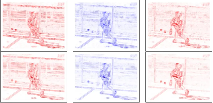
frames are frames 743, 744 and 745 in the tennis sequence. The middle red

im-ages are theMG−₍_x,_y₎=_max

θ{MG−(x,y, θ)}andMG+(x,y)= maxθ{MG+(x,y, θ)}

from Sundberg et al. while the middle blue image isMG(x,y)= maxθ{MG(x,y, θ)},

also from Sundberg et al. The benefits of combingMG−and MG+is to

elim-inate the double boundaries to obtain the correct motion gradient result is

ob-vious. The bottom three images are our motion gradient results (provided here

for comparison purposes), the bottom red images areMG−(x,y) andMG+(x,y)

while the bottom blue image is MG+(x,y). The radius r was 7 and binning

value was 11 with soft binning being used. . . 36

3.11 The top three images (a)-(c) are the motion gradient images for MG−, MG

andMG+for the bench sequence using soft binning. The bottom three images

(d)-(f) are the motion gradient images for MG−_, _MG _and_MG+_{for the rocking}

horse images sequences, also using soft binning. . . 37

3.12 The top three images from left to right are the motion gradient images forMG−,

MG and MG+ for (a)-(c) the hand sequence, (d)-(f) for the Hamburg taxi

se-quence and (g)-(i) for the trees sese-quence. Histogramming was done using soft

binning. . . 38

4.1 (a) shows one of Berkeley Segmentation Dataset (BSDS300) benchmark

orig-inal image, (b) shows the maximum response output by thegPb boundary

de-tector using UC Berkeley gPb MatLab source code and (c) shows the UCM

algorithm output using thegPbresult as input. Note that all regions are closed. 41

4.2 Results for thegPbdetector provided UC Berkeley Computer Vision Group’s

MatLab source code [18]. The top images, (a) to (c), are original images.

The bottom images are the maximal response result of gPb detector over all

orientations for (d) the 744th _{image of tennis sequence, (e) the 10}th _{image of}

the rocking horse sequence and (f) the 10th_{image of bench sequence. . . 44}

(11)

Group [18]. (a) 744 frame of tennis sequence, (b) the 10 image of the

rock-ing horse sequence, (c) the 10th_{image of the bench sequence, the UCM}

bound-ary map for the tennis image after thresholding (d) by 0.1 and (g) by 0.4, the

UCM boundary map for the rocking horse image after thresholding (e) by 0.1

and (h) by 0.4 and the UCM boundary map for the bench image after

thresh-olding (f) by 0.1 and (i) by 0.2. . . 45

4.4 The UCM boundary detection results produced from the 3rdand 4thbench with

thresholding 0.2. We can see a spurious protrusion on the bench’s end and for

the 4th_{image and additional small closed region on the left. . . 46}

4.5 These results are generated by thegPb-UCM algorithm and ourmgalgorithm.

The top images are output of original algorithm, (a) is the gPb result for the

10th_{frame of the rocking horse image sequence while (b) is the UCM result on}

the image in (a). The bottom images are output ofgPb+mg-UCM algorithm,

which is generated by combining ourmgalgorithm withgPb-UCM algorithm.

The bottom left (c) is thegPb+mgresult of the rocking horse image (we just

added ourmgresult to thegPb) while (d) is the UCM result usinggPb+mgas

input. . . 47

4.6 These are results are generated using gPb + mg and UCM algorithms. The

(a)-(c) images are gPb +mg results of the tennis (frame 744), rocking horse

(frame 10) and the bench (frame 10) image sequences. The (d)-(f) images are

the UCM outputs usinggPb+mg(in (a)-(c)) as inputs. The (g)-(i) images are

boundaries and closed regions results for these images after thresholding at 0.5

(tennis), 0.8 (rocking horse) and 0.2 (bench). . . 49

4.7 (a) and (b) are original Tai Chi diagram and rocking horse groundtruth images

while (c) and (d) are the floodfilled output images. Each region is painted with

a different color. . . 50

(12)

and (d) are floodfilled region maps, again the regions are painted with different

colors. . . 51

4.9 (a) is boundary image generated by thresholding the UCM output ongPb+mg,

(b) motion feature image usingδEquation (4.14) and (c) f image using

Equa-tion (4.15). . . 54

4.10 (a) is region map generated by our floodfill algorithm colored in Matlab jet(255)

colormap using the occlusion boundary computed bygPb+mgfor the rocking

horse. We color the boundaries as white while the different regions have

dif-ferent (non-white)colors. (b) This boundary detection result is generated by

using Equations (4.16) and (4.17). we assign boundaries to the regions with

the smaller distance and color it in that region’s color. . . 56

4.11 (a) is boundary image generated by computing the UCM output on gPb+mg,

(b) the motion feature image usingδgiven in Equation (4.14) and (c) is the f

image using Equation 4.15. . . 56

4.12 (a) is region map generated by our floodfill algorithm colored in the Matlab

jet(255) colormap using the boundary computed by gPb+mg. We color the

boundaries white while coloring the regions non-white. (b) This result is

gen-erated using Equations (4.16) and (4.17). We assign boundaries to regions with

4.13 (a) is boundary image generated by computing the UCM output on gPb+mg,

(b) the motion feature image usingδgiven in Equation (4.14) and (c) is the f

image using Equation (4.15). . . 57

4.14 (a) is region map generated by our floodfill algorithm colored in the Matlab

jet(255) colormap using the boundary computed by gPb+mg. We color the

boundaries white while coloring the regions non-white. (b) This result is

gen-erated using Equations (4.16) and (4.17). We assign boundaries to regions with

(13)

(b) the motion feature image using δ given by Equation (4.14) and (c) the f

4.16 (a) is region map generated by our floodfill algorithm, colored by the

Mat-lab jet(255) colormap using the boundary computed by gPb. We color the

boundaries white while different regions are colored in different (non-white)

colors. (b) is the result generated by using Equations (4.16) and (4.17), we

assign boundaries into regions with the smaller distance and color it in that

region’s color. . . 59

4.17 (a) is boundary image generated by computing the UCM output based ongPb,

4.19 (a) is boundary image generated by computing the UCM output based ongPb,

(14)

our floodfill algorithm, colored using the Matlab jet(255) colormap using that

boundary. We color the boundaries white while different regions are colored

with different (non-white) colors. . . 61

4.22 (a) is the optical flow estimation using Brox et al. while (b) is new estimated

optical flow using our 1st order method. We show the optical flow in every

region in different colors. We can see that the affine model result is a smooth

optical flow for each region. . . 62

4.23 (a) is new estimated optical flow using our 1st order method overlaid on the

original image, with white pixels indicating the detected boundaries. (b) is new

optical flow at the boundaries colored with the regions’ colors they belong to

with white pixels indicating the detected boundaries. (c) and (d) show the same

flow fields as in (a) and (b) but they are overlaid on the colored regions map. . . 63

4.24 (a) and (b) are new estimated optical flow using our 1st and 2nd order method

while every region colored by region color so as to observe the performance

inside regions. . . 65

4.25 (a) is new estimated optical flow using our 2nd _{order method overlaid on the}

original image with white pixels indicating the detected boundaries. (b) is new

optical flow at the boundaries boundaries, colored by the regions’ colors that

they belong to, again with white pixels indicating the detected boundary pixels.

(c) and (d) are (a) and (b) but with optical flow overlaid on the colored regions

map. . . 66

5.1 (a) is boundary image output by using the UCM algorithm for the tennis image

and (b) is regions map generated by our floodfill algorithm. . . 67

(15)

the 1 order estimated optical flow overlaid on the original image and on the

regions image. (d) and (e) are 1st_{order estimated optical flow at the boundaries}

displayed on the original image and regions map. The boundaries are colored

white. . . 68

5.3 (a) is colored Brox et al. optical flow for the tennis image. (b) and (c) is

the 2nd _{order estimated optical flow overlaid on the original image and on the}

regions image. (d) and (e) are 2nd_{order estimated optical flow at the boundaries}

white. . . 69

5.4 (a) is boundary image output by using the UCM algorithm for the bench image

and (b) is regions map generated by our floodfill algorithm. . . 70

5.5 (a) is colored Brox et al. optical flow for the bench image. (b) and (c) is

the 1st _{order estimated optical flow overlaid on the original image and on the}

regions image. (d) and (e) are 1storder estimated optical flow at the boundaries

white. . . 81

5.6 (a) is colored Brox et al. optical flow for the bench image. (b) and (c) is

the 2nd order estimated optical flow overlaid on the original image and on the

regions image. (d) and (e) are 2nd_{order estimated optical flow at the boundaries}

white. . . 82

5.7 The left column images are warping error images of Brox et al.’s method, The

middle column images are warping error images of 1storder method, The

mid-dle column images are warping error images of 2nd _{order method, They are}

computed on rocking horse, tennis and bench sequences. . . 83

(16)

image. (d) is the Brox et al. reconstructed image, (g) is the 1 order

recon-structed image and (j) is the 2nd_{order reconstructed image. (b), (e), (h) and (k)}

are the respective images for the tennis image while (c), (f), (i) and (l) are the

respective images for the bench image. . . 84

5.9 (a), (d) and (g) shows the rocking horse images in rectangle [80 80 480 460],

(b), (e) and (h) show the tennis image in rectangle [70 180 360 360] and (c), (f)

and (i) show the bench images in rectangle [1 100 190 320]. The top images are

for Brox et al., the middle images are for the 1st order method and the bottom

images are the 2nd _{order model. The rectangles in red indicate the region of}

interest. Each image shows the RMS warping error for that image. . . 85

5.10 We see some difference in our 1st_{and 2}nd_{results of tennis image on the ground}

pats. Here we also show their difference in rectangle [250 1 360 360]. . . 86

5.11 From top to bottom are the reconstructed images using Brox et al.’s method and

our 1stand 2nd order method for each region’s warping errors displayed for the

rocking horse image. . . 87

5.12 From top to bottom are the reconstructed images using Brox et al.’s method and

our 1st_{and 2}nd _{order method for each region’s warping errors displayed for the}

bench image. . . 88

A.1 These are results output by the UCM algorithm. The top images are original

images. The upper middle images are the output of the gPb algorithm for

6th_{image of hand image sequence, the 10}th_{image of the Hamburg taxi image}

sequence and 10thimage of the trees image sequence. The lower middle images

are the UCM results usinggPb. The bottom images are the segmentation results

for the UCM algorithm usinggPbwith thresholding at 0.8, 0.8 and 0.4 for the

3 image sequences. . . 91

(17)

images sequence, the 10 image of Hamburg taxi image sequence and of 10

image of the trees image sequence. The middle images are UCM results using

gPb+mgfor the 3 images. The bottom image are the segmentation results of

the UCM algorithm usinggPb+mg with thresholding at 0.9, 0.9 and 0.6 for

the 3 images. . . 92

A.3 Sundberg et al.’s results for 6th_{image the hand sequence, including}δ_, _f_{, region}

map and distance assignment to regions. . . 93

A.4 Sundberg et al.’s results for the 10th _{image of the Hamburg taxi sequence,}

in-cludingδ, f, region map and distance assignment to regions. . . 94

A.5 Sundberg et al.’s results calculated on 10th_{image of the trees sequence,}

includ-ingδ, f, region map and distance assignment to regions. . . 95

A.6 Top flows: 1storder optical flow for the 6thimage of hand sequence, for colored

optical flow. Middle and lower flows: 1st _{order flow overlaid on the original}

image and the region map colour by the color of the region the flow vector are in. 97

A.7 Top flows: 2nd_{order optical flow for the 6}th_{image of hand sequence,for colored}

optical flow. Middle and lower flows: 1st _{order flow overlaid on the original}

image and the region map colour by the color of the region the flow vector are in. 98

A.8 Top flows: 1storder optical flow for the 10thimage of Hamburg taxi sequence,

for colored optical flow. Middle and lower flows: 1st_{order flow overlaid on the}

original image and the region map colour by the color of the region the flow

vector are in. . . 99

A.9 Top flows: 2nd order optical flow for the 10thimage of Hamburg taxi sequence,

for colored optical flow. Middle and lower flows: 2ndorder flow overlaid on the

original image and the region map colour by the color of the region the flow

vector are in. . . 100

(18)

uncolored and colored optical flow. Middle and lower flows: 1 order flow

overlaid on the original image and the region map colour by the color of the

region the flow vector are in. . . 101

A.11 Top flows: 2ndorder optical flow for the 10thimage of trees sequence, for both

uncolored and colored optical flow. Middle and lower flows: 2nd _{order flow}

overlaid on the original image and the region map colour by the color of the

region the flow vector are in. . . 102

A.12 The warping errors calculated on hand sequence. The top images use Brox et al

optical flow while the middle images use 1st order flow and the bottom images

2ndorder flow. . . 103

A.13 The warping errors calculated on Hamburg taxi sequence. The top images use

Brox et al optical flow while the middle images use 1st order flow and the

bottom images 2nd order flow. . . 104

A.14 The warping errors calculated on trees sequence. The top images use Brox et al

optical flow while the middle images use 1st order flow and the bottom images

2ndorder flow. . . 105

A.15 1st _{order method’s optical flow overlaid on the bench images from 006 to 013. . 107}

A.16 1st order method’s optical flow overlaid on the rocking horse images. . . 108

A.17 1st order method’s optical flow overlaid on the tennis images from 740 to 747. . 109

A.18 2nd_{order method’s optical flow overlaid on the bench images from 006 to 013. . 110}

A.19 2nd_{order method’s optical flow overlaid on the rocking horse images. . . 111}

A.20 2ndorder method’s optical flow overlaid on the tennis images from 740 to 747. . 112

(19)

3.1 These data are computed on 2.4 Ghz Intel Core i7 processor and 8 GB 1600

MHz DDR 3 Memory. . . 33

5.1 We perform warping error calculation for: the 10th_{image of the rocking horse}

sequence and bench sequences and the 744thimage of the tennis sequence for

the Brox et al., 1st_{order and 2}nd_{order flow fields. Zero flow means using vector}

(0,0) to compute warping errors as upper bound. Figure 5.7 shows the warping

error images. . . 72

5.2 We perform Structural Similarity Index (SSIM) calculation for: the 10thimage

of the rocking horse sequence and bench sequences and the 744thimage of the

tennis sequence for the Brox et al., 1st_{order and 2}nd_{order flow fields. . . 73}

5.3 We perform warping error calculation for 3 red rectangles in: the 10th _image

of the rocking horse sequence and bench sequences and the 744th_{image of the}

tennis sequence for the Brox et al., 1st order and 2nd order flow fields. Zero

flow means we use vector (0,0) to compute warping errors as upper bound. . . . 73

5.4 Region warping errors calculated by using Brox et al., 1st order and 2nd order

methods for the 10th_{rocking horse image. . . 74}

5.6 Region warping errors calculated by using Brox et al., 1st _{order and 2}nd _order

methods for the 744th_{tennis image. . . 79}

5.5 Region warping errors calculated by using Brox et al., 1st _{order and 2}nd _order

methods for the 10th_{bench image. . . 80}

(20)

burg taxi sequence and he 10 of trees sequence. . . 96

A.2 Individual region warping errors calculated for Brox et al. and 1st _{and 2}nd

optical flow for 6thimage of the hand sequence. . . 96

A.3 Individual region warping errors calculated for Brox et al. and 1st and 2nd

optical flow for 10th_{image of the Hamburg taxi sequence. . . 106}

A.4 Individual region warping errors calculated for Brox et al. and 1st and 2nd

optical flow for 10thimage of the trees sequence. . . 106

(21)

Introduction

In this thesis, we investigate some newest and best approaches for the calculation of boundary

detection and optical flow fields, in particular for those boundaries that are occlusion

bound-aries. Occlusion occurs when one object with a distinct motion passes over another object with

a different distinct motion. We would like to measure optical flow for these two objects, right

up to the occlusion boundary that separates them. Towards our goal, we implement Sundberg

et al.’s occlusion boundary algorithm [44] that uses optical flow to detect and label occlusion

boundaries as occluding or occluded. This chapter explains some common concepts about

op-tical flow, discontinuous opop-tical flow at occlusion boundaries and why we need to do boundary

detection before (or at the same time) computing optical flow.

1.1 Optical Flow

Optical flow is the apparent motion of image pixels from one image to the next in a sequence

of images. 2D optical flow is the perspective projection of the relative 3D motion between

an observer and the scene. We use the word “apparent” to denote our assumption that

inten-sity changes between images is due entirely to the motion captures between the two images.

Scene illumination changes are assumed not to happen or to happen so slowly that the effect

is negligible over two frames. Scenes are assumed not to have uniformly textured objects (or

(22)

assumed to only have local uniformity) as such images can undergo motion but not exhibit any

illumination changes.

We use vector fields to display this motion. Each vector indicate the direction and the speed

of every pixel in the image. Some researchers use colour images because there is no need to

subsample or scale the flow field. However, we find that subtle optical flow changes, such as

those at an occlusion boundary, are not well displayed by such images.

Our datasets are from the University of California Berkeley Computer Vision Group

Web-site ([18] and Stein and Hebert [40]), including the tennis, rocking horse, bench, hand,

Ham-burg Taxi (made by Nagel’s research group) and Trees (made by Shakey the Robot at Carnegie

Mellon University) image sequences.

Many algorithms for estimating optical flow, from the classical methods proposed by Horn

and Schunck [24] or Lucas and Kanade [30], both in 1981, to more modern approaches such

as the hierarchical regularization method by Brox et al. [9] have been proposed. Consider the

10th _{frame of the rocking horse image sequence and its Brox et al. optical flow as shown in}

Figure 1.1. Our Brox et al. implementation was first implemented in C by Md. Faisal in 2007

[14]. He was able to obtain the same optical flow field as Brox et al. did for the Yosemite

sequence. Later, this C code was converted to MatLab. As Figure 1.1 shows, we get some very

good optical flow inside the horse’s head and at some (mostly right) parts of the background,

but optical flow at occlusion boundaries and inside small occlusion regions is not very smooth.

A lot of optical flow work have been done in past, including two classical algorithms by

Horn and Schunck (1981) [24] and Lucas and Kanade (1981) [30]. These algorithms have good

overall performance. However, the optical flow quality is especially poor at occlusion

bound-aries. Optical flow at occlusion remains an open research area. In this thesis, we approach

this problem by using not only an optical flow estimation method but also boundary detection.

We first compute optical flow using the Brox et al. state-of-the-art algorithm [9], which is still

considered one of the best algorithm for the estimation of optical flow. We often show the

optical flow overlaid on the images so that the reader can see exactly how good optical flow

(23)

(a) (b)

Figure 1.1: (a) The 10th frame of rocking-horse sequence from the rocking horse sequence [40] and (b) its optical flow field using Brox et al.’s optical flow algorithm [9] (vectors subsampled by 15 and scaled by 5.0) as implemented by Faisal and Barron [14]. 10 levels were used in the pyramid.

and display optical flow in each region using the regions’ colours.

In this thesis, occlusion boundary detection, is especially important. We wish to compute

optical flow right up to occlusion boundaries, where the optical flow on both sides of the

bound-ary are distinct and correspond to the unique image motions on each side of the boundbound-ary. We

use Maire et al.’s work [31] and Arbelaez et al.’s work [3, 4] to do boundary detection. They

developed a statistical probability map to indicate the probability of a pixel being a boundary

pixel or not.

Our method for recalculating optical flow at occlusion boundaries is based on the Brox et

al. optical flow algorithm we already have. We take Brox et al.’s flow as the original optical

flow and then compute new optical flow based on it and boundaries produced by Maire et

al.’s boundary detection algorithm. The reason we take boundary information into account

is to improve the performance of optical flow at occlusion boundaries. We believe occlusion

boundaries and their closed regions should have significant influence on the flow of all pixels

inside such region. In particular, optical flow at an occlusion region should not “bleed” into

adjacent occlusion regions. We do our experiments on three main image sequences:

(24)

2. the rocking horse and benchmark image sequences from Stein and Herbert [40] and

3. other image sequences (such as the Hamburg taxi sequence and the Shakey the robot

sequence) that we have. These will be present in the appendices.

1.2 Discontinuous Optical Flow At Boundaries

The estimation of optical flow at occlusion is still an unsolved problem in Computer Vision.

Optical flow at occlusion boundaries should exhibit discontinuities caused by moving objects

or a foreground object moving against the background. Obviously, this happens a lot in natural

images, where some objects moving differently pass over each other (occlude each other).

Traditional optical flow algorithms do not work well in these areas. This is because when

there are overlapping motions, many assumptions used by these techniques (for example, Horn

and Schunck’s assumption that the flow field varies smoothly everywhere) are invalid. Zhang

and Barron [49] investigated some newer optical flow methods specifically designed to work

with occlusion. They found these algorithms indeed work better at occlusion boundaries but

still exhibit many of the same kind of problems, but at a smaller scale. In this thesis, we

follow their advice and do boundary detection first before estimating optical flow and which

boundaries are occlusion boundaries. Sundberg et al.’s method [44] uses boundary detection

and Brox et al. optical flow to determine which boundaries are occlusion boundaries. They

never explicitly looked at the optical flow quality at and around these edges. The purpose of

this thesis is to implement various algorithms extending from the idea proposed by Sundberg

et al. [44] to improve optical flow at occlusion boundaries. We believe this will improve the

performance of optical flow at boundaries. Also we will show results computed on different

sequences, including tennis court, rocking horse, benchmark, trees and taxi sequences and

reconstruct the first image from our optical flow and the second image to calculate quantitative

evaluation numbers by comparing the first image and the reconstructed image (via a norm of

(25)

1.3 Thesis Contributions

This thesis makes three contributions:

1. We have implemented Sundberg et al.’s occlusion detector motion gradient algorithm

introduced in [44]. This gradient is used as another channel for boundary detector. We

refer it as the motion cue. Traditional boundary detector typically doesn’t utilize

mo-tion informamo-tion. In this case, having video or momo-tion sequences, we can derive more

information such as motion gradient used in boundary detection as another cue for the

boundary detector.

2. Having these boundaries (closed occlusion contours), we try different methods to

recal-culate optical flow on boundaries and closed regions to produce a better results, including

a first order derivatives, i.e. an affine model, described by Sundberg et al. [44] and a

sec-ond order derivatives quadratic model (we added this model to the flow calculation). We

are trying to use these closed boundary detection outputs to get better estimations of

optical flow.

3. We compute a series of optical flow of image sequence to generate an optical flow video,

which clearly show the object’s motion. Because we are focusing on the estimation of

occlusion boundaries, we can think of various ways to estimate and describe the image

motion at an occlusion boundary. Here we compute continuous optical flow sequences

and put them together in order to generate a movie.

1.4 Thesis Outline

This thesis is organized as follows. Chapter 1 introduces the thesis. We introduce optical flow

at occlusion. The contributions of the thesis plus an overview of its contents are given. We

also explain various concepts, such as motion gradient, globalized probability of boundary,

Orientated Watershed Transform and Ultrametric Contour Map. In Chapter 2, we present a

(26)

detector’s output to improve an optical flow calculation and we give a description of Brox et

al.’s optical flow estimation method [9]. The Chapter 3 describes what a Motion Gradient is

and how it is computed, how to use thePbdetector approach to calculate motion gradient (mg).

We also show all results of our implementation and give the necessary details to explain how

we implement this algorithm. In Chapter 4, we will introduce some other libraries we used in

this thesis. Since we need to usegPb-UCM contour output as our input to generategPb+mg

UCM edge map, we give a description of it, introducinggPband UCM. Also in Chapter 4, we

introduce our own optical flow improvement algorithms; recalculated optical flow results of

different image sequences are shown. Also we show the optical flow results using 1st _{and 2}nd

order models here. The remainder of experimental results are shown in Chapter 5. We evaluate

our results quantitatively and qualitatively, comparing them to many other results. In Chapter

(27)

Literature Survey

This chapter provides a general review of some work related to optical flow estimation and

boundary detection. Optical flow is widely used in the Computer Vision field, for motion

estimation and object detection, among other things. In this thesis, we will need to use a

boundary detector in addition to computing optical flow. Thus, we also review some classic

and common boundary detectors.

In Chapter 1 we discussed how discontinuities are common in natural image sequences and

why this effects the accuracy of optical flow estimation. Many techniques have been proposed

to estimate optical flow while preserving discontinuities in recent several years. We introduce

some classical 2D optical flow methods in this chapter, including the algorithms by Horn and

Schunck (1981) [24] and Lucas and Kanade (1981) [30] as well as other algorithms.

2.1 Classical Optical Flow

In Computer Vision, the estimation of optical flow is still a challenging problem, especially

optical flow at occlusion boundaries. Barron et al. [6] and Fortun et al. Fortun-et-al-2015 have

summarized various techniques for estimating optical flow. Most of these different optical flow

algorithms are based on the motion constraint equation (sometimes also called the optical flow

constraint line), which constrains the correct velocity at a pixel with spatio-temporal gradients

(28)

ofIx,Iy andIt to fit a line defined by these parameters, as shown in Equation (2.1).

Ixu+Iyv+It = 0 (2.1)

Figure 2.1: Motion flow Constraint Equation (from [7]).

In Figure 2.1, the normal velocityv⊥is defined as the vector perpendicular to the constraint

line, which means is the velocity with the smallest magnitude on the motion constraint line.

This equation is one linear equation in two unknowns,uandv. That is to say, only the motion

component in the direction of the local gradient of the image intensity may be estimated. This

is called the aperture problem [7]. Here ˜v⊥ = v⊥nˆ can be computed solely in terms of the

intensity derivatives,Ix, IyandIt as:

v⊥ =

−It

||∇I||₂ and nˆ = ∇I

||∇I||₂,yielding : (2.2)

˜v⊥ =v⊥nˆ =

−It∇I

||∇I||2₂ (2.3)

˜v⊥is the raw normal velocity and∇I =(Ix,Iy) is the spatial intensity gradient.

Pioneering optical flow algorithms were proposed by Horn and Schunck [24] and Lucas

(29)

2.1.1 Horn and Schunck Optical Flow

Horn and Schunck [24] combine the motion constraint equation (in Equation 2.1) with a global

smoothness term to constrain the estimated velocity field to vary smoothly everywhere:

||∇u||2₂+||∇v||2₂. (2.4) Horn and Schunck minimize:

Z

D

∇IT ·~v+It 2

+α2

||∇u||2₂+||∇v||2₂dxdy, (2.5) where domain D means the whole image. The magnitude ofαindicates the influence of the

smoothness term (also known as the Lagrange multiplier) relative to the motion constraint

equation. Typically,αcan range from 1.0 to 10.0 to 100.0.

We can minimize the Equation (2.5) :

f(x,y,u,v,ux,uy,vx,vy)=(Ixu+Iyv+It)2+α2(u2x+u 2 y +v

2 x+v

2

y) (2.6)

to derive two iterative Gauss-Seidel equations, themselves in turn derived from the

Euler-Lagrange equations of Equation (2.6):

un+1 = u¯n− Ix

h

Ixu¯+Iyv¯+It i

(α2+_I2 x +Iy2)

and (2.7)

vn+1 = v¯n− Iy

h

Ixu¯+Iyv¯+It i

(α2+_I2 x +Iy2)

. (2.8)

wherendenotes the iteration number,u0_and_v0_{denote initial velocity estimates, which are set}

to zero, and ¯un_{and ¯}_vn_{denote 3}_×_{3 neighbourhood weighted averages of}_un_and_vn_.

The problem with Horn and Schunck optical flow at occlusions can be attributed to the

global smoothness constraint. Optical flow tends to “bleed” over occlusion boundaries. That

(30)

when the two regions have different motion and thus an occlusion edge exists between them.

Such optical flow is very inaccurate.

2.1.2 Lucas and Kanade Optical Flow

Lucas and Kanade [30] assume constant velocity in local neighbourhoods and solve:

           u v            =            P iI2xi

P iIxiIyi

P

iIxiIyi PiIyi2           

−1           −P iIxiIti

−P iIyiIti

           (2.9)

with the sums running fromi=1 ton. Sometimes, the derivatives are weighed by valuesWithat

are inversely proportional to the distance of a pixel from the center pixel. A Gaussian function

is typically used to compute such values. From empirical observations [6] it was found that

Gaussian weights only improved the solution a negligible amount.

2.2 Refined Optical Flow

Some researchers have developed algorithms to estimate optical flow at occlusion. Most of

these algorithms are based on Horn and Schunck and Lucas and Kanade classical methods we

presented in the previous 2 subsections. For example, Yuan et al. [47] proposed a method

based on Horn and Schunck’s model while Niu et al.’s [35] proposed a method based on Lucas

and Kanade’s model. Both of these algorithms get better results over their original methods.

However, they still have problems at occlusion, as we will discuss below. Zhang and Barron

[49] implemented these two methods in 2D and 3D. Here, we focus on the 2D algorithms.

2.2.1 Yuan et al.’s Optical Flow

Yuan et al. [47] investigated a modification of Horn and Schunck’s method with a variable

weighting coefficient, a modified mean template based on intensity differences and a more

(31)

tested their modified algorithm on real image sequence and compare their results with Horn and

Schunck’s results under the same conditions. Their results shows that the modified algorithm

performs better than Horn and Schunck’s model in dealing with discontinuities at occlusion

boundaries. The experimental results also showed that the compensating iterative algorithm is

more efficient than the Gauss-Seidel iterative algorithm.

This new approach mainly focused on the adjustment of the weight coefficient, which

modi-fies Horn and Schunck’s method and leads to a better preservation of flow discontinuities. Yuan

et al.’s computation include:

1. Yuan et al. adopt variable smoothing weight coefficient instead of the constant coefficient

αin the energy function.

2. a new mean template is used to calculate the average value of velocities which is more

accurate compared to the symmetric template used by Horn and Schunck.

3. the Gauss-Seidel method is replaced by a new and more efficient iterative method to

solve the Euler-Lagrange equations.

2.2.2 Niu et al.’s Optical Flow

Niu et al. [35] refined the flow estimate in a continuous region using the temporal

neighbor-hood’s data while the flow estimate in a discontinuous region was computed using the local

motion boundary information. They presented a dynamic over-constrained system of

equa-tions for dense, accurate flow computation to recover the optical flow and its deformation and

acceleration. They compared their results with the results obtained by the optical flow fields

obtained by Lucas Kanade [30] and others. The comparison demonstrated the expected

accu-racy of the proposed dynamic over-determined method by selective use of pixels in a point’s

spatial and temporal neighborhood.

The Lucas and Kanade constant flow methods described above solves an overdetermined

system by the least squares solution. However, that solution is robust to Gaussian noise but

(32)

object boundary or an occlusion boundary. It is obvious that in such cases, the constant flow

model is invalid. In Lucas and Kanade, the pixels within a neighborhood used to estimate

optical flow are not selected, rather all pixels in the neighborhood are used.

Niu et al. [35] have devised a dynamic overdetermined optical flow solution with the goal

of computing dense, accurate flow estimates with well preserved motion discontinuities. That

is to say, their system avoids regularizing the irregular pixels, the outliers, and preserve

discon-tinuities. To do so, they construct a dynamic overdetermined system of equations to recover

optical flow and its deformation and acceleration. The main ideas of this technique can be

described in the following steps:

1. Build up the initial equations at each pixel from selected pixels in its spatial

neighbor-hood.

2. Test the obtained flow vectors using the brightness constraint equation.

3. Refine the flow vectors with selected temporal neighbors.

4. Detect possible occlusion or disocclusion regions with the help of acceleration vectors.

2.2.3 Qualitative Comparison of Horn and Schunck’s, Lucas and Kanade,

Yuan et al. and Niu et al. Optical Flow

We ran Horn and Schunck, Lucas and Kanade, Yuan et al. and Niu et al. on the rocking horse

image sequence. However, we do not show these flows because the image motion is too fast

and the intensity derivatives are aliased. Poor flow fields result. Unfortunately we do not have

access to hierarchical implementations of these methods. Brox et al. is a hierarchical method

and with 10 levels it can measure this motion. For 1 level (no pyramid used) it cannot measure

good flow, like these 4 methods. More details on Brox et al.’s performance for the rocking

(33)

2.3 Brox et al. Optical Flow

Many researchers, such as Sundberg et al. [44] (Brox is a co-author) believe that “variational

optical flow is most accurate on edges”. A prominent variational optical flow method in that of

Brox et al. [9]. Indeed this is the optical flow method used by Sundberg et al.

Brox et al. [9] proposed a hierarchical variational optical flow method. This method has

produced the best optical flow for Yosemite Fly-Through sequence. The energy term of this

variational method extends that of Horn and Schunck, by making constancy assumptions not

only on brightness but also on the spatio-temporal gradient. Their method combines three

assumptions: a brightness constancy assumption, a gradient constancy assumption and a

spatio-temporal smoothness constraint, all using a coarse-to-fine warping strategy to measure larger

optical vectors. Faisal and Barron [14] provided an implementation and evaluation of this

algorithm in C. The assumptions:

1. The Brightness Constancy Assumption requires that the grayvalue of a pixel not be

changed by the displacement of a pixel with velocity (u,v) from timettot+1 :

I(x,y,t)= I(x+u,y+v,t+1). (2.10)

This assumption uses the motion constraint equationIxu+Iyv+It =0.

2. The Gradient Constancy Assumption requires that the spatial gradients of at a pixel be

constant over time:

∇I(x,y,t)= ∇I(x+u,y+v,t+1). (2.11) Here∇=(∂x, ∂y)T is for the spatial gradient.

3. The Smoothness Assumption assume a piecewise smooth flow field, which can be

ex-pressed as:

|∇3u|2+|∇3v|2, (2.12)

(34)

for the optical flow calculation,∇₃ turns into the spatial gradient.

4. The Multiscale Approach requires an image pyramid be built for the 2 images one is

computing optical flow for. The image reduction factor between levels in the pyramid is

η(we useeta = 0.95 in this thesis). The idea is that image reduction over a number of

pyramid levels slows down the image velocity magnitude. For example, with 10 levels

and eta = 0.95, a 1 pixel/frame image velocity at level 1 becomes 0.6 pixels/frame at

level 10. The coarse to fine strategy for computing fast optical flow (that would otherwise

be aliased) requires a warping step at each level in the processing. The idea is to warp

the computed optical flow out of the image at each level. Subsequent level optical flows

only reflect the “corrected” optical flow needed to register the images. The sum of all

these flows is the final flow.

Brox et al.’s energy model as proposed in [9] can be written as:

E(w)=

Z

ωΨ

((I(x+w)−I(x))2)dx+γ Z

ωΨ

(|∇I(x+w)− ∇I(x)|2)dx+α Z

ωΨ

(|∇₃u|2+|∇₃v|2)dx

(2.13)

whereΨ(s2) =

√

s2+2 _using_L1 _{functionals is a convex robust minimizer.} _{is a very small}

positive constant that preventsΨfrom being 0. Brox et al. choose = 0.001. αis a

regulariza-tion parameter which determines the smoothness of the output.

We minimize E(w) by using the Euler-Lagrange equations and numerical approximation

methods. They solve this nonlinear system of equations using SOR iterations. In order to

estimate large displacement, they use the pyramid structure to downsample the images. The

system of equations is solved in each level to get successive approximations of the optical flow.

Note that we still have some problems in the computation of optical flow at occlusion

boundaries. From Stein and Herbert and Sundberg et al. ’s work we can see that occlusion

boundary detection is an important step in the estimation of boundaries’ optical flow.

In this thesis, we use a MatLab implementation of Faisal and Barron’s C code [14] of the

(35)

pyramid with 10 levels. At each level in the pyramid we save the full optical flow computed at

that point. We end at level 1, with the final optical flow,uandv.

Figure 2.2 shows the optical flow results at levels 10 to 2 while Figure 2.3 shows the final

optical flow at level 1 for the 10th_{frame of the rocking horse sequence.}

level 10 level 9 level 8

level 7 level 6 level 5

level 4 leval 3 level 2

Figure 2.2: Level 10 to level 2 Brox et al. optical flow using coarse to fine pyramidal structure [9] for the 10thframe of the rocking horse sequence.

Since the correct optical flow is unknown, direct quantitative analysis is not possible. To

perform indirect quantitative analysis we compute warping error. Given two images, I1 and

I2, and the optical flow,v = (u,v), we usevandI2 to reconstructI1. The norm of the squared

difference between the originalI1and the reconstructedI1is due to either error in the computed

(36)

pixel (i, j) with floating point image velocity (u,v) we need to compute the pixel intensity at

(i+ u, j +v) and copy it to the reconstructed I1. To do this, we need to interpret the pixel

values at the 4 interger positions surrounding this pixel at (b(i+u),c(j+v)), (d(i+u),c(j+v)), (b(i+u),e(j+v)) and (d(i+u),e(j+v)). We use bilinear interpolation via MatLab’sinterp2

function. Figure 2.4.

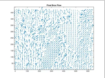
Figure 2.3: The final optical flow field for the 10th_{frame of the rocking horse image sequence.}

We also try to run Brox et al.’s method using 1 level shown in Figure 2.5. Aliased flow is

true for other methods and that they need to be in a hierarchical framework like Brox to handle

fast image motions.

The Brox et al. optical flow method returns a good estimation of optical flow. The major

shortcoming of the algorithm is that it does not perform well at occlusion boundaries or at areas

inside regions formed by closed occlusion boundaries. One idea we investigate in this thesis

is to estimate optical flow independent inside each closed occlusion region. We need to do

boundary detection and region detection to find all these locations before further processing.

(37)

(a) (b) (c)

Figure 2.4: (a) and (b) are the 10thand 11st rocking horse images used for optical flow calcu-lation while (c) shows the reconstructed 10th _{image using the 11}st _{image and the optical flow}

at frame 10 (see Figure 2.3). Qualitatively, we can see the reconstructed and original rock-ing horse images look the same. Quantitatively, the warprock-ing error is 0.104764, which is quite small.

Figure 2.5: The optical flow for the 10th _{frame of the rocking horse image using Brox et al.’s}

method using 1 level.

(38)

2.4 Optical Flow and Occlusion

A complete (as of 2011) of the many approaches to computing optical flow at occlusion are

given in an MSc thesis [48] and a conference paper [49]. We repeat here (next paragraph)

verbatim the survey in the conference paper [49] and then add our contributions at the end.

Nagel [34] has proposed an “oriented smoothness” constraint that tries to suppress

optical flow propagation in the direction orthogonal to the occluding boundaries in

an attempt to stop velocity smoothing across motion boundaries. Bruhn etu al. [11]

presented a variational method to compute optical flow in real-time using

bidirec-tional multi-grid strategies. Their energy functional regularizes a data term and an

enhanced HS smoothness constraint that uses piecewise smoothness on both the

image intensity distribution and the computed flow. Deriche et al. [13] imposes

two conditions on the flow to allow discontinuities in the solution: isotropically

smoothing the optical flow field inside homogeneous regions and preserving the

flow discontinuities in the inhomogeneous regions by smoothing along curves with

constant flow but not across them. Heinrich et al. [21] used a variational

formu-lation where discontinuities are preserved by non-quadratic regularization using a

modifiedLp _{norm. Schn¨orr [38] explicitly represented discontinuities by}

separat-ing the stationary environment and movseparat-ing object and then estimatseparat-ing flows over

these separate domains. Heitz and Bouthemy [22] used a multi-modal,

coarse-to-fine approach in a global Bayesian decision framework to estimate flow while

preserving occlusion discontinuities. Guichard and Rudin [19] used the divergence

of the flow and modelled occlusion using intensity-based matching and magnitude

of divergence constraints. Ghosal and Van˘ek [17] used a ’weighted anisotropic’

smoothness term where locations with little available gradient information are

more constrained and locations with strong intensity gradients (potential motion

discontinuities) are less constrained. Proesmans et al. [36] computed flow

(39)

bound-aries is non-linearly fed back to the computed flow, preserving the discontinuities.

[45] proposed a framework that simultaneously detects flow boundaries and uses

those results in flow estimation. Flow analysis for basic Horn and Schunck, Horn

and Schunck with boundary detection, edge-based flow estimation with boundary

detection and edge-based flow estimation with boundary detection and a

projec-tion method were presented. G¨uler and Derin [20] detect discontinuities in noisy

and textured images using weak continuity (using an elastic membrane energy

model) and line configuration constraints in an graduated non-convexity

optimiza-tion framework.

One item for future work in Zhang’s thesis [48] is to detect closed occlusion boundaries

first, as described by Stein and Herbert [40] and Sundberg et al. [44] and then compute robust

regularized flow within each closed occlusion boundary segment. Both Stein and Herbert and

Sundberg et al. used optical flow in their occlusion boundary detection schemes but optical flow

was only used to compute and label occlusion boundaries as either occluding or occluded. One

interesting thing about Sundberg et al.’s work is that they detect closed occlusion boundaries

(suggesting that optical flow could be computed inside such regions independently of optical

flow elsewhere).

Note that occluded pixels have no correspondence in consecutive frames, and pixels in

occluded regions may be overlaid by moving objects which can not be observed.

Optical flow estimation for images exhibiting both small and large displacements addressed

by Brox and Malik [10] and Strecha et al. [41]. Because adjacent motions can differ so

sig-nificantly, obviously there must be an occlusion boundary between them, although Brox and

Malik do not explicitly compute such boundaries. Their algorithm combines correspondence

with the Brox et al. [9] optical flow framework. Ayvaci et al. [5] consider occlusion detection

as a variational optimization problem based on Lambertian reflection and static illumination

assumptions. To detect moving objects or occlusion layers, their method optimizes the relaxed

cost function using convex minimization. Bleyer et al. [8] combine image segmentation and

(40)

[28] utilize graph-cuts to handle occlusions, but they do it properly. They suggest that one

pixel should correspond to at most one pixel in another image which is logical and

reason-able. Heitz et al. [23] propose a multi-modal approach to solve the estimation of optical flow

by using various complimentary constraints. They say multiple constraints will improve the

accuracy of the estimation. Some work utilizes machine learning techniques to do boundary

detection including Jacobson et al. [27] and Humayun et al. [25].

Fortun et al. [16] propose two steps to handle occlusion in the estimation of optical flow:

1. occlusion detection and

2. occlusion filling.

We address these two steps in the next two subsections.

2.4.1 Occlusion Detection

The occlusion detection process, for example, uses detectors to find boundaries and regions

to segment the image into occluded and non-occluded regions. There is some work using this

step to do optical flow estimation, such as Stein and Herbert [40], Sundberg et al. [44] or Ince

and Konrad [26]. We discuss the work of Stein and Herbert [40], Sundberg et al. [44] in two

subsections below.

First, these methods assume the existence of occlusions. Traditional methods for handing

occlusion estimated optical flow ignoring occlusion, then identified occlusion boundaries and

corrected optical flow in these areas. However, Ince and Konrad suggested interacting between

optical flow and occlusion estimation to do this correction by using a variational formulation.

They showed this extrapolation could lead to significant improvements in the estimation of

optical flow over other approaches. Mozerov in [33] considered the estimation of optical flow

as a matching problem and solved it by global optimization. Their approach to this goal used

a pre-estimation of optical flow to correlate motion vectors frame by frame. Based on Brox et

al.’s work [9], Li et al. [46] used an extended framework, refined based on coarse-to-fine

(41)

large displacements. They supplied local motion candidates then combined them to estimate

global optical flow in a second step. They used a global regularized energy optimization to do

the aggregation step. Other work was based on a Bayesian framework, such as Strecha et al.

[41] and Smith et al. [39]. Also both Smith et al. [39] and Sun et al. [42, 43] utilized layered

model techniques.

2.4.2 Occlusion Filling

Fortun et al. distinguish between occlusion detection, i.e. segmenting the image into occluded

and non-occluded regions, and occlusion filling, i.e. recovering the missing flow subfields

in occluded regions. One suggestion to do this is to turn off the data term in the variational

calculation and just compute a smoother flow estimnate for this region (since it is occluded

we cannot see it). In this thesis, we do not try to estimate the optical flow for occluded parts

of the image that cannot be seem. Rather, we are interested in computing optical flow in all

visible regions, especially right at moving occlusion boundaries, where potentially 2 surfaces

(the occluded and the occluding) have different motions.

2.5 Stein and Herbert Occlusion Boundaries

Stein and Herbert [40] initially over-segmentated the image and then with the help of a

bound-ary detector, identify occlusion boundaries. They provided a global reasoning model by

learn-ing the notion of fragment connectivity and constructlearn-ing a factor graph to model fragment and

junction independences. They also provided some examples to compare the results of using

appearance cues only to those using both appearance and motion cues. Their results show

that appearance and motion classification performed together gave better results for fragment

detection and occlusion boundary detection. Stein and Herbert also provided a few occlusion

boundary detection examples that had consistently poor performance using their approach, due

to the extremely harsh lighting and the lack of texture. Finally, they proposed to extend their

(42)

reference frame in a short video clip.

2.6 Sundberg et al.’s optical flow

Sundberg et al. [44] propose a method of utilizing optical flow for occlusion boundary

detec-tion. Their work is based on thegPb-UCM technology and Brox et al.’s optical flow. They used

a motion gradient algorithm to derive motion information from several frames to improve the

boundary detector’s performance. Also they developed a strategy to decide which boundaries

are occlusion boundaries using boundary detector’s output and optical flow data. In order to

transform optical flow data into boundary information, they proposed a weighted least square

approach to recalculate optical flow and then, by comparing the difference in the flow at each

side of a boundary pixel to decide if that boundary pixel lies on the occlusion boundary.

Sundberg et al. report better occlusion boundary results than the boundary detector without

motion information (in this case, we cannot distinguish between occlusion and non-occlusion

boundaries). Inspired by their results, we decided to utilize their boundary detector output to

improve the optical flow in the closed regions bounded by occlusion boundaries. We have

implemented their motion gradient algorithm. We also utilize theirgPbboundary detector and

UCM to produce closed boundaries. Given such regions, we the recompute optical flow within

each region using the original Brox et al. optical flow.

Originally, the idea was to detect closed occlusion boundaries first. Both Stein and

Her-bert [40] and Sundberg et al. [44] suggested to combine boundary detection and optical flow

together to generate better results. Both of them used optical flow in their occlusion

bound-ary detection schemes, but they did not show any optical flow results in their papers. Indeed,

Sundberg et al. only compute optical flow for a small area around hypothesized occlusion

boundaries. In the following chapters, we will introduce our implementation of the motion

(43)

2.7 Large Displacement Optical Flow

Brox and Malik proposed a method in [10] by combing various descriptors with the variational

optical flow approach together to estimate optical flow. Also they developed a way to introduce

features matching technique into optical flow field. The variation approach uses coarse-to-fine

warping technique to compute the velocity, however, it is a kind of relaxing processing which

will return incorrect optical flow at dense parts. They estimate large displacement optical flow

using descriptor matching to improve the accuracy of dense optical flow. They use different

terms such as color, gradient, matching and descriptors in their energy model. They perform

region matching based on regions produced by segmentation method using SIFT and color

descriptors. While these descriptors are computed in histograms of oriented gradients (HOG).

Then they use continuation method to minimize the energy equation. The large displacement

(44)

Motion Gradient

In the previous chapter, we presented many concepts about the estimation of optical flow.

Dis-continuous optical flow is a common phenomenon in natural images, these disDis-continuous may

be caused by moving objects or partially occluded objects. Some optical flow methods

fo-cus on distinguishing occlusion boundaries from other boundaries. Stein and Herbert [40] and

Sundberg et al. [44] try to detect the occlusion boundaries with the help of a boundary

detec-tor generated by combining motion cues, static cues and optical flow together. An evaluation

of optical flow methods with energy terms to account for occlusions by Zhang and Barron

[49] leads to the conclusion that detecting occlusion boundary can play an important role in

estimation of the optical flow at occlusion boundaries.

Both Stein and Herbert and Sundberg et al. present algorithms for occlusion boundary

detection that uses optical flow. Neither actually show the computed optical flows for their

oc-clusion regions (regions with closed ococ-clusion boundaries). Sundberg et al. use an additional

motion cue, the motion gradient and with the information provided by the UCM boundary

de-tector and the variational optical flow method by Brox et al. [9] they detected closed occlusion

boundaries. They determined whether a boundary was an occlusion boundary by

threshold-ing the difference between optical flow in the two adjacent regions: if the two optical flow

were significantly different an occlusion boundary was hypothesized. Finally, they assigned

figure/ground labels to these boundaries by comparing the optical flow on the boundary points