Parameterization-based tracking for the P2 experiment
IuriiSorokin1,2,afor the P2 collaboration
1Institute for Nuclear Physics, University of Mainz, Germany 2PRISMA Cluster of Excellence
Abstract.The P2 experiment in Mainz aims to determine the weak mixing angleθW at low momentum transfer by measuring the parity-violating asymmetry of elastic electron-proton scattering. In order to achieve the intended precision ofΔ(sin2θ
W)/sin2θW =
0.13% within the planned 10 000 hours of running the experiment has to operate at the rate of 1011detected electrons per second. Although it is not required to measure the
kinematic parameters of each individual electron, every attempt is made to achieve the highest possible throughput in the track reconstruction chain.
In the present work a parameterization-based track reconstruction method is described. It is a variation of track following, where the results of the computation-heavy steps, namely the propagation of a track to the further detector plane, and the fitting, are pre-calculated, and expressed in terms of parametric analytic functions. This makes the algorithm ex-tremely fast, and well-suited for an implementation on an FPGA.
The method also takes implicitly into account the actual phase space distribution of the tracks already at the stage of candidate construction. Compared to a simple algorithm, that does not use such information, this allows reducing the combinatorial background by many orders of magnitude, down toO(1) background candidate per one signal track. The method is developed specifically for the P2 experiment in Mainz, and the presented implementation is tightly coupled to the experimental conditions.
1 The P2 experiment
1.1 Motivation
One of the fundamental parameters in the Standard Model is the weak mixing angleθW, which defines
the relative strength of the electromagnetic and weak interactions. The weak mixing angle is a scale-dependent quantity and it has been measured at various energies and in different processes [1] (Fig. 1). However, the most precise measurements, performed at the Z pole, are marginally consistent, and the measurements at lower energies are not precise enough to discriminate between the Standard Model and possible extensions. The P2 experiment in Mainz aims at measuring the weak mixing angle at low momentum transfer (average momentum transfer squaredQ2=4.5·10−3GeV2/c2) to a precision
of 0.13%. Such measurement will be a stringent test of the Standard Model, and has the potential of discovering physics beyond the Standard Model in the running.
2 <(F7>
TJOƿ8 2 28 "17
28 F 28 Q
-&1
4-% 1!.&4"
.PMMFS 2XFBL
40-*%
/V5F7
F%*4 5FWBUSPO "5-"4
$.4 IT
Figure 1. Scale dependence of sin2θW together with completed (black error bars) and planned (blue error bars, value chosen to coincide with theory) experimen-tal measurements [1].
Figure 2.CAD model of the P2 detector.
1.2 The method and the setup
In the P2 experiment the weak mixing angle is going to be determined from the parity-violating asymmetry of elastic electron-proton scattering. The latter can be related toθWas follows:
APV= σσL−σR
L+σR =
GFQ2
4√2πα(QW+F(Q
2)), (1)
QW=1−4 sin2θW, (2)
whereAPV is the parity violating asymmetry,σLandσR are the elastic scattering cross-sections for
left- and right-handed electrons,QWis the weak charge of the proton,F(Q2) is the Fermi constant,α
is the fine structure constant, andQ2is the momentum transfer squared.
The planned experimental setup is shown in Fig. 2. A longitudinally polarized electron beam is scattered in a liquid hydrogen target, and the current of the elastically scattered electrons is measured with a Cherenkov Detector. The beam polarization is flipped with a rate of several kHz. Providing the integrated luminosity with both helicities is the same, the parity violating asymmetry can be evaluated as:
APV =
NL−NR NL+NR,
(3)
where theNLandNRare the number of detected electrons with left-handed and right-handed helicities
respectively.
AsAPVis on the order of 10−8, to achieve the required statistical precision ofΔAPV ≤6·10−10, the number of detected electrons needs to be higher than 3·1018. In order to collect such immense
statistics on a feasible timescale, assuming 10 000 running hours, the experiment needs to work at a rate of 1011detected electrons per second.
The long (60 cm) target is also necessary to achieve the required event rate. A vast amount of bremsstrahlung photons is produced in the target, creating a background in the Cherenkov Detector. The lead shield in the middle of the setup blocks the photons coming directly from the target, but still a considerable amount of the photons hit the Cherenkov Detector after a Compton scattering in the inner surface of the magnet. The superconducting magnet bends the electrons around the shield.
Evaluating the weak mixing angle from equation 1 requires knowing the distribution of the mo-mentum transfer squaredQ2. Because of the considerable energy loss and multiple scattering in the
target, theQ2 distribution need to be determined from a detailed simulation. Here one can not fully
rely on GEANT4, as the precise shape of the scattering distribution is important, and helicity corre-lated effects are not implemented. To properly tune and validate the simulation the Tracking System is necessary.
1.3 Tracking system
The main purpose of the Tracking System is to help evaluating theQ2 distribution of the primary
electron-proton scattering. In addition, the Tracking System is going to be used for detector align-ment, as well as for monitoring the experimental conditions by means of watching the kinematic distributions.
TheQ2distribution needs to be determined with the relative systematic uncertainty on the mean
below 0.2%. The measurement will be performed at a decreased beam rate, to reduce the effect of combinatorial background. With the same data sets the detector alignment and validation of the magnetic field map will be performed.
During the normal experiment operation, at the full beam rate, the amount of data, produced by the Tracking System will be too large to be processed with the affordable computing resources. The data will be acquired in short intervals, with sufficient pauses for processing in between. Every attempt is made to achieve the highest possible throughput in the reconstruction chain, as this would result in better sensitivity to variations of the experimental conditions. The minimum required duty cycle can not be quoted at the moment, as it depends on the tracking performance and details of experimental conditions.
The Tracking System will be based on the MuPix [4] high-voltage monolithic active pixel sensors (HV-MAPS). MuPix features high rate capability (2 MHz/chip tested, 284 MHz/cm2 theoretical),
time resolution of about 11 ns, low mass, low power consumption (300 mW/cm2), and high efficiency
(99.5%) [4]. The chip was originally developed for the Mu3e experiment [7], and fits very well to the needs of P2.
The sensors will be arranged in four planes. The choise of four planes was made to minimize the material budget. At least three planes are necessary to constrain the track parameters within a magnetic field, and at least one more is needed to distinguish between the real tracks and random hit combinations. The planes are placed in pairs, with 2 cm distance between the planes within each pair, and 54 cm between the pairs (Fig. 3). Placing the planes close to each other reduces the area to search for the matching hit, hence reduces the combinatorial background. Yet, a certain spacing is necessary to accurately measure the track curvature.
1.4 Reconstruction challenge
The major challenges in track reconstruction are the extreme track rate, high hit density, and consid-erable background from the bremsstrahlung photons. For the first estimates it was assumed that the track reconstruction is done in 45 ns time frames, which corresponds approximately to four times the time resolution of the MUPIX chip (measured to beσt=11 ns[4]). At the full beam rate this leads to about 800 reconstructible signal electrons and up to 6000 background hits per plane in one frame.
Obviously, at such high rates, the reconstruction has to be done on-line. To achieve the highest possible throughput the reconstruction is considered to be implemented on a FPGA. For this a fast and simple algorithm is required, such as the parameterization-based tracking.
1.5 Simulations
In the following sections references to the GEANT4 [5] simulations will be made. At present the GEANT4 model of the P2 experiment includes most of the relevant material in the detector, uses a realistic magnetic field map, and considers the relevant electromagnetic processes. The major simpli-fications in the model are that: (a) the incident beam is stationary, and goes along the z-axis, whereas in fact it is planned to scan with the beam over the target volume in order to prevent the target from boiling, (b) that the tracking planes are flat, without any dead area, whereas in fact they will consist of 2x2 cm2 sensors, overlapping in x and y (because of the dead edges), and interleaved in z, and
(c) the misalignment and the uncertainty on the field map are not simulated. The present model is adequate for evaluating the performance of the tracking algorithm. Further extension of the model are necessary for other studies, as will become clear from the text.
2 Parameterization-based tracking
2.1 Concept
The presentedparameterization-based trackingis a variation oftrack following. Track following is a track reconstruction method, when first track seeds are constructed, and then hits from the consequent planes are added to the seeds one-by-one. Finally, the constructed hit combinations —track candi-dates— are fitted, and the best candidates are selected based on the fit quality information, usually
χ2.
In P2 the reconstruction goes backwards: each hit in plane 3 (Fig. 3) is taken as a track seed, and then hits from the planes 2, 1 and 0 are added in the respective order. A combination of one, two, or three hits, constructed in such way, will be called atrack segment.
To decide which hits can be added to a track segment one needs to extrapolate the segment to the next (upstream) plane. The extrapolated position, along with the extrapolation uncertainty, define the
region of interest(ROI) — the region where all hits match to the track segment. Usually, there is more than one hit in the ROI. In such case extended segments are constructed with each of the matching hits.
In the parameterization-based tracking the ROIs are pre-calculated beforehand, and expressed in terms of parametric functions of the coordinates of the segment hits. So, during the reconstruction, the optimal ROI can be easily evaluated from the parameterizations for any track segment.
In the current implementation, for the sake of simplicity, the ROIs are chosen to be rectangular. The characteristics of the rectangular ROI, namely the x- andy-positions, the x- and y-sizes, and the rotation are expressed as 3rd order polynomial functions of the segment hit coordinates. In the following these quantities will be referred to asxpos,ypos,xsize,ysize, andθrotrespectively. How exactly xpos, ypos, xsize, ysize, and θrot depend on the coordinates of the segment hits will be explained in
section 2.3. The variablesxpos,ypos,xsize,ysize, andθrotexpress the position of the ROI respectively to
the last hit in the segment, in a rotated reference frame, as shown in Fig. 4. The 3rd order polynomials were chosen also for simplicity, and planned to be replaced with splines in the future. Also, for technical reasons, in the current implementationθrotis always zero, which also needs to be fixed.
The next section (2.2) will describe how to define the ROI for a given track segment. In section 2.3 it will be shown how to proceed from a set of segments with defined ROIs to the sought parameter-izations. In sections 2.4 and 3.3 it will be demonstrated that not only the ROIs, but also the track parameters, such as the position and the momentum, can be parameterized.
Target
beam 2 cm 2 cm
54 cm B
z
R
Electron trajectory
Hit 1
Hit 0 Hit 2 Hit 3
Plane 0 Plane 1 Plane 2 Plane 3
Figure 3. Schematic zR-view on the target and the tracking planes.
Figure 4. Schematic xy-view on the target and the tracking planes.
2.2 Defining the region of interest
In this work the ROIs are defined by comparing the segments with reference tracks. The reference tracks are either tracks from the GEANT4 simulation, or high quality (lowχ2) tracks, reconstructed
from the low beam rate experimental data. At low beam rate the combinatorial background is small, so track candidates can be constructed with a simple exhaustive search, and a conventional rigorous fit of every candidate can be performed.
reference tracks selected in this way, it is trivial to define the ROI: it is the region, where the selected reference tracks are concentrated. In the current implementation it is defined as the rectangle of the minimal area, which encloses not less than a certain fraction (typically 95%–99%) of the reference tracks. Obviously, the ROI, defined in such way, will enable to find only these tracks, for which similar reference tracks were available. To go beyond this limitation one can scale up the size of the obtained ROI.
2.3 Parameterizing the region of interest
First the general form of the parameterizations need to be defined. As mentioned in section 2.1, in the current implementation the ROIs are chosen to be rectangular, so one needs to define five functions:
xpos,ypos,xsize,ysize, andθrot.
The functions were chosen to be 3rd order polynomials, and must depend on the coordinates of the segment hits. But using the coordinates of all hits explicitly is disadvantageous because this would make the parameterization functions to be up to six-dimensional, which would later on lead to certain technical difficulties. The number of variables can be reduced by taking one symmetry and one correlation into account.
First the functions for the ROI in plane 2 (Fig. 3) will be defined. The ROI in plane 2 can depend only on the coordinates of the hit in plane 3. Since the position of the ROI is defined relativeley to the last hit of the segment (hit 3), and due to the rotational symmetry of the setup, the functionsxpos,ypos, xsize,ysize, andθrotcan be defined as functions of the radial position of hit 3,R3, only (Fig. 4).
The ROI in plane 1 can depend only on hits in planes 3 and 2. Again, due to the rotational symmetry, the functionsxpos,ypos,xsize,ysize, andθrotcan be defined to depend only onR3and on the
relative position of hits 2 and 3,ξ32andη32(Fig. 4).
The ROI in plane 3 should, in general, depend on position of hits in planes 3, 2, and 1. But the positions of hits 3 and 2 become strongly correlated as soon as the position of hit 1 is fixed. Indeed, the
x- andy-position of hits 1 and 3, together with the target, make a coarse constraint on the track radius, whereas thezpositions of the two hits, together with the defined track radius, constrain the track inclination w.r.t. to thexy-plane. Even the coarse constraints on the track parameters lead to a strong correlation between hits 3 and 2 because the planes are very close to each other. Therefore, in the current implementation the position of hit 2 is ignored. Taking into account the rotational symmetry, the functionsxpos,ypos,xsize,ysize,θrotare defined to depend onR3, as well as on the relative position
of hits 1 and 3,ΔR31 andΔφ31 (Fig. 4). Here polar coordinates are chosen because they are less
correlated.
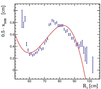
Next step is to find the coefficients of the functionsxpos,ypos,xsize,ysize,θrot. This is done by fitting
the functions to ROIs, created from the reference tracks as follows. The phase spaces of the param-eterization functions,{R3}in case of plane 2,{R3, ξ32, η32}in case of plane 1, and{R3,ΔR31,Δφ31}in
case of plane 0, are divided in bins. All reference tracks are grouped according to each of the three binnings. For each bin in each phase space a ROI is created using the reference tracks in this bin (an example is shown in Fig. 5). The ROIs give the fit points for the functions: the center of the respective bin gives the coordinates of the point, and ROI characteristics, namely the size, the position and the rotation, give the point values. An example fit of one of the parameterization functions,xsize(R3) for
the ROI in plane 2, is shown in Fig. 6.
2.4 Parameterization of track parameters
−1 −0.5 0 0.5 1 1.5 2 1
− 0.9 −
0.8 −
0.7 −
0.6 −
0.5 −
0.4 −
0.3 −
0.2 −
0 20 40 60 80 100 120 140 160 180 200
ξ32[cm]
η32
[c
m]
N
umb
er
o
f r
ef
er
en
ce
tr
ac
ks
Figure 5. Spatial distribution of the reference tracks in plane 2 w.r.t. to the hit in plane 3 in the R3 bin
[73.5; 74.5) cm. The coordinates are explained in Fig. 4, as well as in the text. Black rectangle is the ROI, evaluated from this spatial distribution. Red rect-angle is the ROI, evaluated from the parameterizations.
R3[cm]
0.
5 ·
xSI
ZE
[c
m]
60 70 80 90 100
0 0.2 0.4 0.6 0.8 1
Figure 6. Fit of the xsize(R3) of the ROIs in
plane 2 with a 3rd order polynomial. The size of the bars is inversely proportional to the weight of the point, which is defined as the number of reference tracks in the bin.
consider the positions of two hits only (necessarily from different plane pairs). Indeed, the curvature of the track is additionally constrained by the position of the target, and the other two hits are strongly correlated with the selected two. For the P2 experiment so far only the parameterization of the abso-lute momentum was implemented. It was chosen to use the hits in planes 1 and 3, and the variables
R3,ΔR31,Δφ31. The results are presented in section 3.3. However, in order to completely replace the
fitting procedure one would need to parameterize theχ2of fit, which necessarily requires considering the positions of all four hits. Whereas using 7 independent variables (two coordinates per hit minus one rotational symmetry) is clearly not possible in the way described above, it might be possible to either use a sophisticated function(s) of the hit coordinates as an argument for the parameterization function, or to develop (adopt) an appropriate method of evaluating the coefficients of the parameter-ization functions, which does not require a 7-dimensional binning. Further studies in this direction have not yet been done, but are planned.
3 Performance tests
A series of tests of the described tracking technique has been performed on the GEANT4-simualted data. Two different data samples were used to create the parameterizations, and to evaluate the per-formance. The samples were created with exactly the same GEANT4 model, as briefly described in the section 1.5.
3.1 Efficiency of the parameterized regions of interest
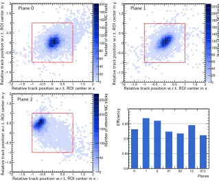
The efficiency of a parameterized ROI is defined as the ratio of the number of signal tracks, that are within the ROI, to the total number of reconstructible signal tracks. A signal track is considered re-constructible if it made a hit in each of the four tracking planes. Only electrons that hit the Cherenkov Detetor are considered as signal. A more illustrative measure of the performance of a parameterized ROI is the distribution of the position of the signal track w.r.t. the center of the ROI. Both measures of ROI performance were evaluated with the current, yet not optimized, configuration of the algorithm.
A set of reconstructible signal tracks was selected, and for each track the ROIs in planes 2, 1 and 0 were constructed. The bottom right bar chart in Fig. 7 shows the fraction of signal tracks within individual ROIs, and ROI combinations. The overall efficiency of constructing track candidates is given by the bin “123”, and equals 91 % in the given case. The inefficiency is caused partially by imperfect parameterization with 3rd order polynomials, and partially by hard bremsstrahlung by the signal electrons.
The three histograms in Fig. 7 show the distribution of the position of the signal track w.r.t. the center of the ROI. The quantity is plotted in the ROI local reference frame (Fig. 4), and in the units of ROI half-size. In such coordinates the tracks inside−1<x<1−1< y <1 are within the ROI.
This test proves the concept of parameterizing the ROIs. Further studies are needed to evaluate the perfomance of this technique.
−2−2 −1.5 −1 −0.5 0 0.5 1 1.5 2 1.5 − 1 − 0.5 − 0 0.5 1 1.5 2 N u m b er of ref e rence M C track s 0 20 40 60 80 100 120 140 160 180 200 Plane 0
Relative track position w.r.t.ROIcenter in x
Re la tiv e tr ac k po si tio n w. r. t. R OI c en te r i n y
−2−2 −1.5 −1 −0.5 0 0.5 1 1.5 2 1.5 − 1 − 0.5 − 0 0.5 1 1.5 2 N u m b er of ref e rence M C track s 0 20 40 60 80 100 120 140 160 180 200 220 Plane 1
Relative track position w.r.t.ROIcenter in x
Re la tiv e tr ac k po si tio n w. r. t. R OI c en te r i n y
−2−2 −1.5 −1 −0.5 0 0.5 1 1.5 2 1.5 − 1 − 0.5 − 0 0.5 1 1.5 2 N u m b er of ref e rence M C track s 0 50 100 150 200 250
Plane 2
Relative track position w.r.t.ROIcenter in x
Re la tiv e tr ac k po si tio n w. r. t. R OI c en te r i n y Planes
0 1 2 01 02 12 012
0.8 0.85 0.9 0.95 1 Effic ie nc
y 1
3.2 Combinatorial background
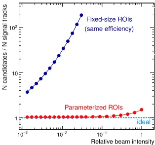
To see whether using parameterized ROIs brings any advantages in performance, a comparison to an algorithm using constant-size ROIs was done. The constant-size ROIs were chosen to be square, their size in planes 0 and 2 was set equal, and the size was tuned to the same efficiency (91%) as was obtained with the parameterized ROIs. The ROI in plane 1 was made so large that all hits from plane 1 were always enclosed (actually, it would be enough to select hits only from the same sector, and not from the whole plane, which would result in factor 4 fewer combinations).
Fig. 8 shows the number of constructed track candidates per one reconstructible signal track using the constant-size and the parameterized ROIs. Clearly, the difference is dramatic. One can expect that after fitting and applying aχ2cut most of the wrong candidates, constructed using the fixed-size
ROIs, will be rejected, and the amount of combinatorial background in the two cases will become very similar. The advantage of using parameterized ROIs is that it eliminates the need to perform the huge number of unnecessary fits.
One has to keep in mind that the parameterization-based tracking implicitly uses the information about the kinematic distribution of the true tracks, whereas the algorithm with the fixed-size ROIs doesn’t.
Relative beam intensity 3
−
10 10−2 10−1 1
1 10 2 10
1 cm 1.5 cm 2 cm 2.5 cm 3 cm
Parameterized ROIs
Fixed-size ROIs (same efficiency)
ideal
N ca
nd
ida
tes
/ N sign
al
tr
ack
s
Figure 8.Number of track candidates, constructed per one reconstructible signal track, using the parameterized ROIs, and using the constant-size ROIs, tuned to the same efficiency.
3.3 Parameterization of track momentum
, [GeV/c] MC )/p MC - p t Relative error, (p 0.1
− −0.08−0.06−0.04−0.02 0 0.02 0.04 0.06 0.08 0.1
Number of tr
ack
s
0 100 200 300 400 500 600
Width = 1.23 % Width = 1.23 % O0set = 0.114 % O0set = 0.114 % Gaussian 0t
par fit
Offset
, [GeV/c]
MC )/p MC - p t Relative error, (p 0.1
− −0.08−0.06−0.04−0.02 0 0.02 0.04 0.06 0.08 0.1
N
u
mber of tr
acks
0 20 40 60 80 100 120 140 160 180 200
Width = 1.40 % Width = 1.40 % O0set = 0.033 % O0set = 0.033 % Gaussian 0t
fi fit
Offset
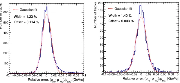
Figure 9.Relative error on the absolute momentum, evaluated from the parameterization (left), and determined with a rigorous GBL fit (right).
4 Summary
The parameterization-based tracking is a variation of track following, where the regions of interest are pre-calculated, and represented as a set of parametric analytic functions of the hit coordinates. In the current implementation the ROIs are defined by comparing the track segment with the reference tracks. Also the track parameters, such as the position and the momentum can be parameterized.
The parameterization-based tracking has been implemented for the P2 experiment and tested on simulated data. The first tests have proven the concept, and demonstrated a great improvement in the number of constructed track candidates, hence required fits, as compared to an algorithm with fixed-size ROIs. The parameterization of the absolute momentum is almost as accurate as the rigorous fit.
References
[1] N. Bergeret al., J. Univ. Sci. Tech. China46, no.6, 481-487 (2016) [2] K. Aulenbacher, AIP Conf. Proc.1563, 5-12 (2013).
[3] R. Bucoveanu, M. Gorchtein, H. Spiesberger PoS LL2016, 061, (2016) [4] H. Augustinet al., Nucl.Instrum.Meth.A845, 194-198 (2017)
[5] J. Allisonet al.Nucl.Instrum.Meth.A835, 186-225 (2016) [6] C. Kleinwort, Nucl.Instrum.Meth.A673107-110 (2012)
![Figure 1.bars, value chosen to coincide with theory) experimen-tal measurements [1].θcompleted (black error bars) and planned (blue error Scale dependence of sin2 WFigure 2](https://thumb-us.123doks.com/thumbv2/123dok_us/8134460.1355748/2.482.47.439.83.227/figure-coincide-experimen-measurements-thcompleted-planned-dependence-wfigure.webp)