Causal diagrams and the logic of matched case-control studies

(1)

Clinical Epidemiology

Causal diagrams and the logic of matched

case-control studies

Eyal Shahar1

Doron J Shahar2 1_{Division of Epidemiology and}

Biostatistics, Mel and Enid Zuckerman College of Public Health, 2_{Departments of Physics and}

Mathematics, College of Science, The University of Arizona, Tucson, AZ, USA

Correspondence: E Shahar

Division of Epidemiology and Biostatistics, Mel and Enid Zuckerman College of Public Health, The University of Arizona, 1295 N Martin Ave, Tucson,

AZ 85724, USA Tel +1 520 626 8025 Fax +1 520 626 2767 Email [email protected]

Abstract: It is tempting to assume that confounding bias is eliminated by choosing controls that are identical to the cases on the matched confounder(s). We used causal diagrams to explain why such matching not only fails to remove confounding bias, but also adds colliding bias, and why both types of bias are removed by conditioning on the matched confounder(s). As in some publications, we trace the logic of matching to a possible tradeoff between effort and variance, not between effort and bias. Lastly, we explain why the analysis of a matched case-control study – regardless of the method of matching – is not conceptually different from that of an unmatched study.

Keywords: causal diagrams, directed acyclic graphs, case-control study, matching, confounding bias, colliding bias, variance

Introduction

“To match or not to match?” is a question that often arises when a case-control study is designed. Unfortunately, neither the logic of matching controls to cases nor the drawbacks of this procedure are widely understood. Sometimes, researchers assume that matching prevents confounding bias by choosing controls that are identical to the

cases with respect to the matched confounder(s).1_{This truth-like argument is almost}

always false. Other times, the true benefit of matching – smaller variance of theoretical estimates – is correctly identified, but the mechanism for such a gain is not explained. Moreover, not many researchers know that matching does not guarantee a tradeoff between effort and variance. The variance is not always reduced in return for the extra effort that should be invested to find matched controls.

We used causal diagrams to demystify the logic and analysis of frequency-matched and individually-matched case-control studies.

Causal diagrams

A full explanation of causal diagrams in the context of bias can be found elsewhere.2

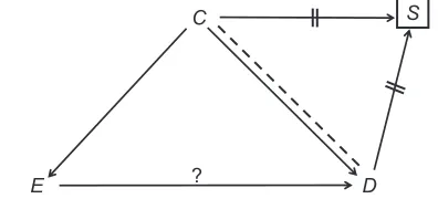
The most relevant ideas are summarized below. We write the names of variables and draw single-headed arrows between causes and their presumed effects (Figure 1). Since a cause always precedes its effects, a loop of self-causation does not exist. The

effect of interest (ED throughout this article) is identified by a question mark above

the arrow (Figure 1).

A natural path between two variables is any sequence of causal arrows – regardless of their directionality – that connects the two, and does not pass more than once

Dove

press

M E T H O D O L O g y

open access to scientific and medical research

Open Access Full Text Article

Clinical Epidemiology downloaded from https://www.dovepress.com/ by 118.70.13.36 on 20-Aug-2020

For personal use only.

Number of times this article has been viewed

This article was published in the following Dove Press journal: Clinical Epidemiology

(2)

through each variable. In Figure 1, for example, E and D

are connected by three natural paths: ED; ECD and

ECSD. A common cause of E and D is called a

con-founder (eg, C in Figure 1). If two arrows on a path point at one variable, that variable is called a collider on the path (because the arrowheads collide there). For instance, S is a

collider on the path ECSD (Figure 1). By definition,

a collider is a common effect of two variables (eg, C and D) – the colliding variables.

We distinguish among three types of natural paths between E and D: causal paths, confounding paths, and colliding paths. A causal path, as its name implies, is any

path by which E affects D. For example, ED (Figure 1);

and EXYD. A confounding path is any path in which

E and D share a common cause (a confounder). For example, ECD (Figure 1); and EXYZD. A colliding path

is any path that contains at least one pair of colliding variables

and their collider, for example, ECSD (Figure 1) and

EXYZD.

The theorems of causal diagrams build a solid bridge between a causal structure and expected associations. Both causal paths and confounding paths contribute to the mar-ginal (crude) association between two variables; they are, therefore, called “open” paths. In contrast, colliding paths are “blocked”; they do not add anything to the association between the variables they connect. Referring again to Figure 1, the marginal association between E and D is the

“sum” of the causal path, ED, and the confounding path,

ECD (Figure 2). The colliding path (ECSD) is

an innocent bystander.

If we estimate the magnitude of the effect of E on

D by their marginal association, the estimator contains

confounding bias – the unwanted contribution of the con-founding path (Figure 2). To get an unbiased estimator of the effect of E on D, the confounding path must be blocked.

All methods to block a confounding path (to deconfound) are based on conditioning, which means (in its basic form) restricting a variable to one of its values. Since a value is not associated with any variable, conditioning dissociates a variable from both its causes and its effects. For example, after conditioning on the confounder C (Figures 1 and 2), it will not be associated with E and D, so the confounding path will no longer exist. As will be seen, however, new paths and new associations might be created.

Figure 3 illustrates the consequences of conditioning, using new notation. Conditioning on S, denoted by a box, dissociates S from its three causes (X, Y, and Z) and its three effects (L, M, and N), and is denoted by two lines over each arrow. But more might happen: under certain

conditions,2_{new associations (denoted by dashed lines)}

will be created between variables that collide at S (that is, between causes of S). As a result, we observe new connecting paths, some of which are composed of dashed lines alone (eg, X--Y, and X--Y--Z), whereas others are

composed of dashed lines and arrows (eg, EX--ZD).

Since both types of paths arose after conditioning, we call them induced paths.

An induced path, just like a natural path, may be blocked or open, depending on whether it contains a collider. For

example, the induced path HI--JKL is blocked – not

contributing to the association between H and L – because the path contains the collider K. All induced paths in Figure 3 are open; they create, or contribute to, the association between the variables they connect. Just like a confounding path, an open induced path between the cause-and-effect of interest

E C

D S

? Confounder

Collider

Figure 1 A causal structure.

Note: Thequestion mark denotes the effect of interest.

E C

D

E ? D

+

Figure 2 Components of the marginal association between E and D.

Note: The question mark denotes the effect of interest.

S

Z

X Y

L

N M

E ? D

Figure 3 Consequences of conditioning on S.

Note: The question mark denotes the effect of interest.

Dovepress

Shahar and Shahar

(3)

(here, E and D) is a source of bias. We call that bias colliding

bias,2_{because the culprit is an open path through colliding}

variables.

Deconfounding in an unmatched

case-control study

With these principles in mind, we first depict the causal structure of an unmatched case-control study, assuming only one confounder (Figure 4, Diagram A). As before, the effect

of interest is the causal path ED.

Imagining all people, let the variable S indicate whether a person is selected for a particular study. Since only the selected people are eventually studied, conditioning on S is built into all research designs (Figure 4, Diagram A). The distinguishing feature of a case-control study is the arrow

DS, which shows that disease status affects selection status:

your chances of being selected into the sample are higher if you have the disease than if you do not have it, at some index time. (This is also true for case-cohort sampling and incidence density sampling). Here, however, conditioning on S carries no consequences for the estimated odds ratio, because no new paths are induced (so long as C does not

modify E’s effect on S).2_{To deconfound, we condition on C}

(Figure 4, Diagram B).

Conditioning, as described so far, is often just the first step in the computation. Rather than estimating the odds ratio for only one value of C, we may estimate the odds ratio for each value of C and compute a weighted average of all the estimates. If E and C are binary variables, the deconfounded estimator of the effect of E is computed as follows:

OR_deconfounded= (w₁OR₁+ w₂OR₂)/(w₁+ w₂) (1)

where OR denotes the odds ratio, w denotes the weight, and the subscript denotes the value (stratum) of C. The classic weights in equation (1) are the inverse of the variances of the

C-specific estimates. Such weights minimize the variance of

the deconfounded odds ratio.

Sometimes, weighting is done on the log scale:

ln(OR_deconfounded) = [w₁ln(OR₁) + w₂ ln(OR₂)]/(w₁+ w₂)

OR_deconfounded= exp {[w₁ln(OR₁) + w₂ln(OR₂)]/(w₁+ w₂)} (2) In equation (2), the classic weights are the inverse of the variances of the log of the C-specific estimates. Those weights minimize the variance of the log of the deconfounded

odds ratio.3

Alternatively, we may condition on C by adding the vari-able to an unconditional logistic regression model:

ln [odds(D = case)] =β0+β1E +β2C

OR_deconfounded= exp(β₁) (3)

Whichever computation is used, deconfounding is a tradeoff between variance and bias, because the variance of the odds ratio always increases after conditioning. If the sample is restricted to only one value of C, the variance increases because the estimate is computed from a smaller sample. That is also the case for deconfounding by a weighted

average or by regression.4_{As far as the variance is concerned,}

breaking the sample and reassembling the pieces does not perfectly restore the intact sample size.

Of course, it is not necessary to compromise the variance. We may keep the sample intact – that is, not condition on the confounder – and tolerate the bias in return for a smaller variance.

Deconfounding in a matched

case-control study

Figure 5 shows the causal structure of a matched case-control

study, under the same conditions and notation: ED is the

effect of interest; C is a single confounder; and S indicates selection status. One theoretical exception aside, a matched design is distinguished from its unmatched counterpart by

the arrow CS. The value of the matched confounder also

E

C

D S

Diagram A

? _E

C

D S

?

Diagram B

Figure 4 Confounding (A) and deconfounding (B) in an unmatched case-control study.

Note: The question mark denotes the effect of interest.

E D

S

?

C

Figure 5 The causal structure of a matched case-control study.

Dovepress Causal diagrams and matched case-control studies

(4)

plays a role in deciding whether a person will be selected into the sample. For instance, a disease-free person will be selected for a 1:1 matched study only if a yet-to-be-matched case shares his (or her) value of C. Similarly, a diseased per-son will not be retained in the sample if no C-matched control is found. That is also true for a frequency-matched case-control study, in which groups of disease-free people are periodically selected to match the distribution of confounders in accumulated groups of cases.

Adding the arrow CS turns S into a collider: CSD

(Figure 5). Following inevitable conditioning on S, an asso-ciation is created between C and D, the colliding variables, and an open induced path now connects the cause-and-effect

of interest (EC--D). Matching not only failed to block a

confounding path, but also added colliding bias (EC--D) on

top of confounding bias (ECD). The magnitude of the net

bias depends on the strength and direction of each path. Before discussing the remedy, and later, the wisdom of matching, an intriguing question might be asked. Having nullified the association between C and D, how can

match-ing result in net bias? Do the paths CD and C--D not sum

to a null association? Figure 6 reveals the answer. The null association between C and D is the sum of three paths – not

two – the third of which is CED. Assuming the effect

CED is not null, the arrow CD and the dashed line C--D do not add up to a null association (Figure 6). Colliding

bias was indeed mixed with confounding bias (Figure 7). We

note, in passing, that matching in a cohort study (CSE)

removes both types of bias, because the associational sum of CE and C--E is null.2

One exception exists, as noted above. The paths CD

and C--D sum to a null association (no net bias), if the

causal path CED is precisely null – that is, no third path

exists. That can happen if E is not a cause of D (Figure 8, Diagram A), or if C is not a cause of E (Figure 8, Diagram B).

In those circumstances, there is no net bias upon matching, although matching is worthless in the second case (C is not a confounder in Diagram B). Notice that if C is a cause of E,

but the arrow CD is absent, matching adds colliding bias in

the absence of confounding bias (Figure 8, Diagram C). Figure 9 shows the simple, standard remedy when matching results in net bias. Conditioning on the matched confounder, C, removes both colliding bias (denoted by the deletion of the dashed line) and confounding bias. Whatever the motivation for matching might be, it has nothing to do with circumventing the need to deconfound: we still have to condition on a matched confounder. Why match, then? Why invest the extra effort that goes along with finding matched controls instead of recruiting unmatched controls?

The answer comes from the domain of variance. Given a fixed sample size, the variance of theoretical estimates from a matched design will often, but not always, be smaller than the variance of estimates from an unmatched design. And even when the variance is reduced by matching, it might not be reduced by much.

E D

C

D C

D

+

?

C

= null

C

D C

D

+

≠ null

If C E D is

not null, then

Figure 6 Contributors to the null association between the confounder (C) and disease status (D) in a matched case-control study.

E

C

D S

? Non-null

association

Figure 7 Colliding bias superimposed on confounding bias in a matched case-control study.

E

C

D S

E

C

D S

?

Diagram A Diagram B

E

C

D S

Diagram C ?

Figure 8 Special cases of matching: no net bias under the precise null (A); no colliding bias in the absence of confounding bias (B); colliding bias in the absence of confounding bias (C).

Dovepress

Shahar and Shahar

(5)

Matching and variance

To follow the logic of matching, we should first recall that the variance of the (log) odds ratio (marginal association) may be estimated as follows:

Var [ln(OR)] = 1/a + 1/b + 1/c + 1/d (4)

where a, b, c, and d are the cell counts in the 2 × 2 table

(cross-classification by E and D, two binary variables). The variance depends, in part, on the ratio (k) of the number of controls (m) to the number of cases (n). Given a fixed number of cases, the larger the number of controls, the smaller the variance by equation (4), because the cell counts

in controls (b, d) are also expected to be larger (b + d = m).

Close to the null (OR = 1), the variance in a large study with

n cases and m = kn controls is approximately (k + 1)/k times the variance in a theoretical study with an infinite number

of controls.5_{For example, with as many controls as cases}

(k = 1), the variance is twice as large, but with four times as

many controls (k = 4), the variance is only 1.25 times larger.

That is not always a good approximation, however – for example, when the odds ratio is large. Unfortunately, no general formula links the variance to k alone.

A case-control study is often designed under two constraints that fix the value of k. All available cases are retained (n), and the sample size (T) is limited due to

cost: k = (T − n)/n. In the absence of confounding, the

causal path ED is estimated by the marginal odds ratio,

and its variance can be reduced only by recruiting more controls (larger k). Later, when k is fixed but deconfound-ing is needed, we will examine another option to reduce the variance – matching.

Again, let C denote a binary confounder (C = 1 or C = 2),

and let k₁ and k₂ denote, respectively, the control-to-case ratio

in the strata C = 1 and C = 2. The variance of the deconfounded

estimator, regardless of matching, is related to the variance of

C-specific odds ratios (Var₁ and Var₂) as follows:6

Var [ln(OR_deconfounded)] = 1/(1/Var₁+ 1/Var₂) (5)

As previously seen, Var₁ and Var₂ are functions, in part, of k₁

and k₂, respectively. In an unmatched design with a fixed k, we

do not control the values of k₁ and k₂, and therefore, we cannot

influence the values of Var₁ and Var₂ which, in turn, determine

the value of Var [ln(OR_deconfounded)]. Most important, k₁ and k₂

are expected to be different if C is a confounder.

To realize the last key point, first consider the associa-tion between C (the confounder) and D (disease status) in an unmatched study. Assuming no confounders, that association

estimates the effect of C on D via the causal paths CED

and CD (Figure 4, Diagram A). Notice that the paths CE

(which is part of CED) and CD also determine the

magnitude of confounding bias for the effect of E on D.2

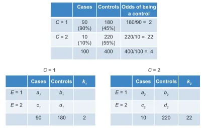
Next, let us consider a hypothetical unmatched study

of 100 cases and 400 controls (k = 4). Suppose that the

estimated odds ratio for the effect of C on D is 11 for the

contrast between C = 1 and C = 2 (Figure 10). Then, the odds

of being a control when C = 2 are eleven times the odds of

being a control when C = 1 (Figure 10). However, the last

statement simply describes the ratio of k₂ to k₁! The

control-to-case ratio in the stratum C = 2 (k₂= 22) is eleven times

that of the ratio in the stratum C = 1 (k₁= 2). We therefore

conclude: the stronger the combined effect of CED and

CD, the larger the difference between k₁ and k₂. And often, though not always, a stronger effect of C on D is accompanied by more confounding bias.

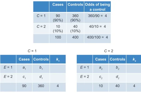
Although matching does not eliminate the need to condition on the confounder, C, it does allow us to

con-trol the values of k₁ and k₂ by forcing the equality k₁= k₂.

If the distribution of C in controls is identical to the distribution of C in cases, the control-to-case ratio will be identical in the two strata of C (Figure 11). Of course, it

E D

S

? C

Figure 9 Deconfounding in a matched case-control study.

Cases Controls Odds of being a control

C = 1 180/90 = 2

C = 2 220/10 = 22 90

(90%) 10 (10%)

100 180 (45%)

220 (55%)

400 400/100 = 4

Cases Controls k1

E = 1 a1 b1

E = 2 c1 d1

90 180 2

C = 1 C = 2

E = 1 a2 b2

E = 2 c2 d2

10 220 22

Figure 10 Association between an unmatched confounder (C) and disease status (top table); counts of cases and controls in C-specific associations of E and disease status (bottom tables).

(6)

will also be identical to the control-to-case ratio in the entire

sample (k₁= k₂= 4).

Why force the equality k₁ = k₂= k? Does that equality

guarantee a smaller variance in a matched design than in an unmatched design of the same size and number of cases? Will the variance expression – equation (5) – be smaller when

k₁= k₂ than when k₁≠ k₂? Unfortunately, the answer is not

unequivocally positive. Often, the variance will be smaller, and sometimes, substantially so. Other times, however, the variance in a matched design will be similar to, or even larger

than, the variance in an unmatched design.5_{Many predictions}

can be made, but no assumption-free algorithm can tell us whether matching will prove to have been the right decision. Despite the intuitive merit in proportionate allocation of controls to the strata of C, the extra effort that matching requires does not guarantee a smaller variance.

Qualifications

In retrospect, it is easy to come up with extreme examples where we can argue in favor of matching. If an unmatched design fails to include controls in one stratum of C, the entire table will be discarded, along with precious cases. Successful matching precludes that situation, but opposing examples also exist. If researchers insist on 1:1 matching, and they fail to find matched controls, precious cases will be discarded, too.

Analysis of matched case-control

studies

Students of epidemiology or biostatistics are taught that a matched design requires a special “matched” analysis, but nothing so far implies anything special about the analysis of a matched case-control study. Indeed, we treat

frequency-matched confounders just as we treat their

unmatched counterparts, using equations (1−3) to

decon-found. For instance, if C1 and C2 are a frequency-matched confounder and an unmatched confounder, respectively, the deconfounded odds ratio may be estimated by the following unconditional logistic regression model:

ln [odds(D = case)] =β0+β1E +β2C1 +β3C2 (6)

The so-called special, “matched” analysis has evolved from technical problems of estimation that arise in indi-vidual matching. But as we will see next, nothing is conceptually different. In individual matching, just as in frequency matching, we still have to condition on the matched confounder(s) to remove the mixture of confound-ing bias and collidconfound-ing bias.

Suppose we have matched one control to each case on a continuous variable – such as weight – and that each case-control pair shares a unique weight. At first glance, it seems that we cannot estimate a deconfounded odds ratio by equation (1) or equation (2), because each stratum of C contains only two people, and therefore, stratum-specific odds ratios cannot be estimated (Figure 12). Equation (3) will also fail because the unconditional

maxi-mum likelihood estimate of β₁ will be biased.7_Nonetheless,

solutions can be found for both a weighted average and regression.

Let a_i, b_i, c_i, and d_i, denote the cell counts in the 2 × 2

table (cross-classification of E and D) in the i-th stratum of C (Figure 12).

With this notation, equation (1) may be generalized as follows:

Cases Controls Odds of being a control

C = 1 360/90 = 4

C = 2 40/10 = 4 90

(90%) 10 (10%)

100 360 (90%)

40 (10%)

400 400/100 = 4

E = 1 a1 b1

E = 2 c1 d1

90 360 4

C = 1 C = 2

E = 1 a2 b2

E = 2 c2 d2

10 40 4

Figure 11 Null association between a matched confounder (C) and disease status (top table); counts of cases and controls in C-specific associations of E and disease status (bottom tables).

CASE CONT

E=1 0 0

E=2 1

1 CASE CONT

E=1 1 1

E=2 0 0 1 1 CASE CONT

E=1 1 1

E=2 0

1 CASE CONT

E=1 0 1

E=2 1 0 1 1 CASE CONT

E=1 0 1

E=2 1 0 1 1 CASE CONT

E=1 0 0

E=2 1 1 1 1 CASE CONT

E = 1 1 1

E=2 0

1 CASE CONT

E = 1 0 1

E=2 0

1 CASE CONT

E = 1 1 0

E=2 0 1 1 1 CASE CONT

E = 1 1 1

E=2 0

1 CASE CONT

E = 1 0 1

E = 2 1 0 Total 1 1 C = 1

C = 2

C = 3

C = 4

C = 5

C = 6

C =

CASE CONT

E = 1 ai bi E = 2 ci di

Ti

C = i

Figure 12 Stratification on the confounder (C) when each matched pair shares a unique value of C.

Dovepress

Shahar and Shahar

(7)

OR w OR w deconfounded i i i i i =

∑

(7) where

OR a c b d

a d b c

i i i

i i

i i

= / =

/

If we use the Mantel–Haenszel weights,8_w

i = bici/Ti

(where T_i= a_i+ b_i+ c_i+ d_i), equation (7) takes the

follow-ing form:

OR a d T

b c T

deconfounded

i i i

i

i i i

i

=

∑

/

/ (8)

Although we derived equation (8) assuming b_ic_i≠ 0, we

may still use it, instead of equation (7), when b_ic_i≠ 0 in some,

but not all, strata of C.

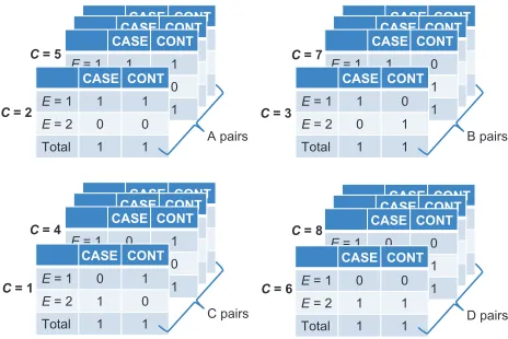
Returning to Figure 12, we observe that T_i= 2 for any

i, and that a_i, b_i, c_i, and d_i take the values 0 or 1. Therefore, we can simplify the computation in equation (8) by group-ing the series of tables in Figure 12 into four types of

case-control pairs, as shown in Figure 13: A-pairs (a_i = 1

and b_i= 1); B-pairs (a_i= 1 and d_i= 1); C-pairs (b_i= 1 and

c_i= 1); and D-pairs (c_i= 1 and d_i= 1). Notice that neither

A-pairs nor D-pairs contribute to equation (8), because the

product of their diagonal cells is zero (a_i d_i= b_i c_i= 0). In

contrast, each B-pair contributes ½ to the numerator of equation (8) (and nothing to the denominator), whereas each C-pair contributes ½ to the denominator (and nothing to the numerator).

Let R and S denote the count of B-pairs and C-pairs, respectively. Then,

OR R

S R S

deconfounded = =

1 2 1 2 /

/ (9)

Equation (9) is called the “matched” odds ratio (often writ-ten as B/C). As we have just realized, however, it is no more than a weighted average of the odds ratio – equation (7) – across the values of C, the matched confounder. Similar

formulae can be developed for 1:k matching (k . 1).

To overcome the sparse data problem in regression, we may fit a conditional logistic regression model, in which the intercept, which is a nuisance parameter in effect estimation, is not estimated. Rather than adding C, the matched con-founder, as a covariate (equation (3)), it is taken into account when the likelihood function is constructed.

If each matched set shares a unique value of the con-founder C, a unique matched set identifier may substitute for C. That is, we may condition on the identifying variable instead of conditioning on C. The same is true in individual matching on several confounders, for example, C1, C2, and

C3, where conditioning on a matched set identifier

substi-tutes for simultaneous conditioning on the three matched variables. Matched sets that share the same values of the matched confounder(s) should be combined under a com-mon identifier.

To summarize, the so-called “matched” analyses are no more than alternative mathematical ways to condition on individually-matched confounders.

Conclusion

As shown here and elsewhere,9–12_{causal diagrams prove to be}

an indispensible tool in research methodology. A few simple principles that connect causation with association were suf-ficient to explain why matching controls to cases not only fails to remove confounding bias, but also adds colliding bias on top of confounding bias. The same principles also show that both types of bias will be removed by conditioning on the matched confounder(s). Tracing the logic of matched case-control studies reveals a possible tradeoff between effort and variance, not between effort and bias. The variance might be reduced in return for the extra effort that matching requires. Of course, the extra effort, if not trivial, may also be invested in recruiting more controls for an unmatched study.

That effort must be invested to gain scientific knowledge is well known, but it is also well known that investing extra

CASE CONT

E=1 1 1

E=2 0 1 CASE CONT E=1 E=2 CASE CONT

E = 1 1 1

E=2 0 0 1 1

A pairs CASE CONT

E = 1 1 1

E = 2 0 0 Total 1 1

CASE CONT

E=1 1 1

E = 1 0 1

E=2 0 0 1 1

C pairs CASE CONT

E = 1 0 1

E = 2 1 0 Total 1 1

CASE CONT

E=1 1 1

E = 1 1 0

E=2 0 1 1 1

B pairs CASE CONT

E = 1 1 0

E = 2 0 1 Total 1 1

CASE CONT

E=1 1 1

E = 1 0 0

E=2 0 1 1 1

D pairs CASE CONT

E = 1 0 0

E = 2 1 1 Total 1 1 C = 1

C = 4

C = 2

C = 5

C = 3

C = 7

C = 6

C = 8

Figure 13 Stratification on the confounder (C) when each matched pair shares a unique value of C, grouping into four possible results.

(8)

Clinical Epidemiology

Publish your work in this journal

Submit your manuscript here: http://www.dovepress.com/clinical-epidemiology-journal

Clinical Epidemiology is an international, peer-reviewed, open access journal focusing on disease and drug epidemiology, identification of risk factors and screening procedures to develop optimal preventative initiatives and programs. Specific topics include: diagnosis, prognosis, treatment, screening, prevention, risk factor modification, systematic

reviews, risk & safety of medical interventions, epidemiology & bio-statical methods, evaluation of guidelines, translational medicine, health policies & economic evaluations. The manuscript management system is completely online and includes a very quick and fair peer-review system, which is all easy to use.

effort does not guarantee a substantial gain, or even any gain, in knowledge. Matching controls to cases is no exception. The merit of matching is often overstated, if not completely misstated.

Disclosure

The authors report no conflicts of interest in this work.

References

1. Bland JM, Altman DG. Matching. Br Med J. 1994;309:1128. 2. Shahar E, Shahar DJ. Causal diagrams and three pairs of biases. In:

Lunet N, editor. Epidemiology – Current Perspectives on Research and

Practice. Rijeka: InTech; 2012:31–62.

3. Kupper LL, Karon JM, Kleinbaum DG, Morgenstern H, Lewis DK. Matching in epidemiologic studies: validity and efficiency considerations.

Biometrics. 1981;37:271–291.

4. Robinson LD, Jewell NP. Some surprising results about covariate adjust-ment in logistic regression models. Int Stat Rev. 1991;58:227–240. 5. Breslow NE, Day NE. Statistical Methods in Cancer Research:

Volume II. Lyon, France: IARC Scientific Publications; 1987.

6. Kahn HA, Sempos CT. Statistical Methods in Epidemiology. New York, NY: Oxford University Press; 1989.

7. Breslow NE, Day NE. Statistical Methods in Cancer Research:

Volume I. Lyon, France: IARC Scientific Publications; 1980.

8. Mantel N, Haenszel W. Statistical aspects of the analysis of data from ret-rospective studies of disease. J Natl Cancer Inst. 1959;22:719–748. 9. Shahar E, Shahar DJ. Causal diagrams and change variables. J Eval

Clin Pract. 2012;18(1):143–148.

10. Shahar E, Shahar DJ. Causal diagrams, information bias, and thought bias. Pragmatic and Observational Research. 2010;1:33–47. 11. Shahar E. A method to detect an unknown confounder: something from

nothing? J Eval Clin Pract. 2012;18(3):702–703.

12. Shahar E, Shahar DJ. Marginal structural models: much ado about (almost) nothing. J Eval Clin Pract. August 23, 2011. [Epub ahead of print].

Dovepress

Dove

press

Shahar and Shahar