Three-dimensional Elastodynamic Modeling of Frictional
Sliding with Application to Intersonic Transition
Thesis by
Yi Liu
In Partial Fulfillment of the Requirements for the Degree of
Doctor of Philosophy
California Institute of Technology Pasadena, California
2009
c
2009
Acknowledgements
I have been exceptionally fortunate to have spent my time as a graduate student working with a number of colleagues who were not only great scientists, but wonderful and interesting people. Now the time has finally come to express my thanks to them.
First and foremost, I would like to express my sincere gratitude to my thesis advisor, Professor Nadia Lapusta, for her guidance, inspiration, and support over years. Nadia introduced me to the field of earthquake mechanics and pointed out interesting problems in this area of research. Na-dia’s patience is remarkable: she is always willing to spend hours with me going through research problems, and help me see connections between seemingly unrelated results and make everything fit together. She has always supported and encouraged me. This thesis would not have been possible without her crucial contribution and insights.
I would like to thank all other members of my committee, Profs. Jean-Philippe Avouac, Kaushik Bhattacharya, Thomas H. Heaton, Ares J. Rosakis, and Guruswami Ravichandran for reviewing my thesis and providing valuable suggestions/criticism. Profs. Bhattacharya and Ravichandran have given me constant support during my study at Caltech and valuable suggestions for my future career development.
lot with computer software and hardware. It was very pleasant to work with Ting Chen and Ajay Harish about numerical algorithms.
I am also indebted to my former advisors Profs. Wei Yang and Keqin Zhu at Tsinghua University. The course Elasticity, taught by Prof. Yang, ignited my initial interest in solid mechanics. Prof. Zhu supervised my undergraduate thesis, which later became my first published scientific paper. It was his encouragement that made me determined to pursue graduate study abroad.
I sincerely appreciate the help and friendship of Xin Guo, Lin Zhu, Zhiyi Li, Fei Wang, Chun-hui Gu, Xiaobai Li, Xiaosong Niu, Ke Wang, Jing Yang, Wei Liang, Li Liu, Jie Chen, Yue Yang, Changling Pang, Tao Liu, Lin Shi, Yue Zhou, Vikram Gavini, Tamer Elsayed, Kook Oh Chang, and many others. They have made my life at Caltech more exciting and wonderful.
Abstract
Spontaneous slip on frictional interfaces involves both short-lived inertially-driven events and long-term quasi-static sliding. An example of considerable practical importance is the response of faults in the Earth’s crust to tectonic loading. The response combines earthquakes that cause destructive ground motions and aseismic slip. Numerical models are needed to study the physics and mechanics of such complex behavior. In part, the models can help understand the observed slip patterns and interpret them in terms of constitutive properties of rocks determined in the lab.
The thesis also develops test problems for dynamic rupture propagation and evaluates simplified quasi-dynamic approaches.
Contents
Acknowledgements iii
Abstract v
Contents vii
List of Figures xi
List of Tables xxv
1 Introduction 1
2 Modeling 3D spontaneous rupture with boundary integral method 10
2.1 Problem formulation . . . 10
2.2 3D boundary integral method . . . 12
2.3 Test problem . . . 16
2.4 Cohesive zone and constraints on discretization . . . 17
2.5 Comparison of numerical results . . . 24
2.5.1 Grid dependence of solutions . . . 24
2.6 Comparison of high-resolution solutions . . . 29
2.7 Discussion . . . 31
2.7.1 Resolution criterion . . . 31
2.7.2 Scale collapse . . . 32
2.7.4 Significance of BI/DFM agreement . . . 34
2.8 Extension to bimaterial fault interface . . . 35
2.9 Conclusion . . . 36
2.10 Appendix: closed-form expression for kernels used for bimaterial faults . . . 37
3 3D modeling of spontaneous earthquake sequences and aseismic slip 39 3.1 Methodology . . . 39
3.1.1 Truncation of elastodynamic response . . . 40
3.1.2 Fault constitutive response: rate and state friction laws . . . 42
3.1.3 Criteria for spatial discretization . . . 45
3.1.4 Computational procedure . . . 46
3.1.5 Model of a strike-slip fault. . . 47
3.2 Simulation example: fault with a homogeneous seismogenic region . . . 48
3.2.1 Parameters of the fault model. . . 48
3.2.2 Fault response: dynamic events and aseismic slip, including transients . . . . 51
3.2.3 Parameters of simulated earthquakes. . . 52
3.2.4 Effect of parameter distributions near the free surface . . . 57
3.3 Parameter validation . . . 59
3.3.1 Spatial discretization. . . 59
3.3.2 Frequency-independent truncation . . . 61
3.3.3 Frequency-dependent truncation . . . 61
3.4 Long-term interaction of slip with compact heterogeneity . . . 62
3.4.1 Supershear burst in the first event . . . 62
3.4.2 No supershear burst in subsequent events . . . 64
3.4.3 Effect of heterogeneity on long-term behavior . . . 65
3.4.4 Fault interaction with heterogeneity of higher normal stress . . . 65
3.5 Comparison of fully dynamic and quasi-dynamic approaches. . . 66
3.5.2 Similarity of quasi-dynamic solutions and their differences with fully dynamic
results . . . 70
3.5.3 Cohesive zone size and numerical resolution in quasi-dynamic simulations . . 72
3.6 Conclusions . . . 73
3.7 Appendix . . . 75
3.7.1 Convolution kernels . . . 75
3.7.2 Updating field variables . . . 77
4 Transition of mode II cracks from sub-Rayleigh to intersonic speeds in the pres-ence of favorable heterogeneity 81 4.1 Burridge-Andrews mechanism on homogeneous fault . . . 81
4.2 Methodology . . . 84
4.3 Advancing main rupture towards a pre-existing subcritical crack: An example of abrupt sub-Rayleigh-to-intersonic transition . . . 87
4.4 Advancing main crack towards a patch of higher prestress: dependence on patch size, prestress, and location . . . 91
4.5 Conclusions and discussion . . . 101
4.5.1 Abrupt change of crack tip speeds . . . 102
4.5.2 Prestress levels for intersonic transition and propagation. . . 103
4.5.3 Transition distance . . . 104
4.5.4 Importance of crack initiation procedure . . . 104
4.5.5 Propagation speeds in the intersonic regime . . . 106
4.5.6 Implications for earthquake dynamics . . . 106
4.6 Appendix . . . 107
4.6.1 Intersonic loading field due to an accelerating sub-Rayleigh mode II crack . . 107
4.6.2 Expressions for stress transfer functional in the spectral boundary integral method . . . 109
5 Intersonic rupture in 3D simulations of earthquake sequences and aseismic slip: effect of rheological boundaries and weaker patches 113
5.1 Fault model . . . 114
5.2 Connection between rate and state friction and linear slip-weakening friction during dynamic rupture . . . 118
5.3 Intersonic transition due to rheological boundaries for Case I of a homogeneous seis-mogenic region . . . 122
5.3.1 Effects of stress concentration at rheological boundaries on intersonic transition126 5.4 Intersonic transition due to favorable compact heterogeneity. . . 130
5.4.1 Weaker patch as favorable heterogeneity for intersonic transition . . . 133
5.4.2 Initiation of secondary cracks in the weaker patch by an intersonic loading field135 5.4.3 Influence of the location of the weaker patch . . . 138
5.5 Discussion . . . 139
5.5.1 Influence of seismic ratio ¯S on rupture behavior. . . 139
5.5.2 Distribution of seismic ratio over seismogenic region . . . 141
5.5.3 Significance of rheological boundaries for rupture dynamics . . . 143
5.5.4 Effect of weaker patches on earthquake sequences. . . 144
5.5.5 Effect of rupture speed on slip distribution . . . 145
5.5.6 On friction behavior during dynamic rupture . . . 146
5.6 Conclusion . . . 147
5.7 Appendix: calculation of horizontal rupture speedc(x, z). . . 148
6 Conclusions and future work 150
List of Figures
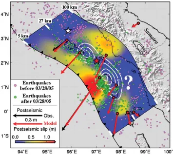
1.1 An example of interaction between earthquakes and aseismic quasi-static slip.
Earth-quakes redistribute stress on faults, causing slow postseismic slip or afterslip in
sur-rounding areas, as shown here on the example of 2005 Nias-Simeulue earthquake in
Sumatra (from Hsu et al., 2006). The postseismic slip, in turn, redistributes stress and
may trigger other seismic events. The figure shows compilation of inferred seismic and
postseismic slip, illustrating the approximately complimentary nature of seismogenic
and aseismic regions. Distribution of seismic slip is indicated by white contours at
intervals of 2 m; color indicates cumulative postseismic slip during the 9 months
af-ter the earthquake. Black and red vectors indicate GPS observations and their match
using the inferred postseismic slip, respectively. White and red stars are epicenters
of 2004 Aceh-Andaman and 2005 Nias-Simeulue earthquakes, respectively. Pink and
green dots denote earthquakes with body wave magnitudemb>4.5 before and after the
2005 event. The regions of high seismicity correspond to the transition between regions
of seismic and aseismic slip. The question mark indicates the region where afterslip
may have occurred but it is not detectable by the existing GPS network. White tick
marks on the northern and southern boundaries of the postseismic slip model indicate
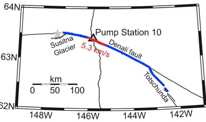
1.2 An example of inferred intersonic propagation in a large strike-slip earthquake. The
2002 Denali (Alaska) earthquake produced a surface rupture of about 340 km (dark
blue line). Modeling of near-fault acceleometer records suggests that the rupture in a
segment of about 40 km (red line) may have propagated with intersonic speeds, with
an average speed of 5.3 km/s (Ellsworth et al., 2004). . . 5
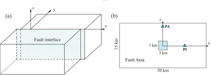
2.1 (a) A planar fault interface (y= 0) is embedded in an infinite uniform elastic medium.
(b) On the fault interface, the square in the center is the nucleation area. The triangles
are the receivers at which we compare time-histories of slip, slip rate, and shear stress.
Relative to an origin at the center of the fault, the receiver PI hasz coordinate 0 km
andxcoordinate 7.5 km, and the receiver PA hasxcoordinate 0 km andzcoordinate
6.0 km. The stress parameters are specified in Table 2.1. . . 12
2.2 Cohesive zone during rupture, along both in-plane and anti-plane directions, for BI0.1
(dashed curve), DFM0.1 (dash-dotted curve), and DFM0.05 (solid curve) solutions . . 23
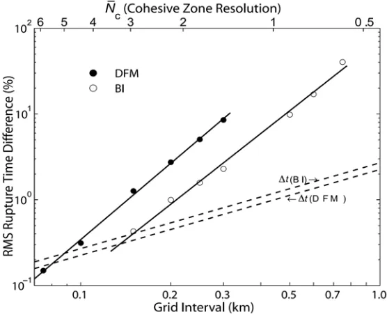
2.3 Differences in time of rupture, relative to reference solution, shown as a function of grid
interval Δx. Differences are RMS averages over the fault plane. Open circles are BI
solutions, relative to BI0.1 (the smallest grid-interval BI case). Solid circles are DFM
solutions, relative to DFM0.05 (the smallest grid-interval DFM case). The dashed
lines show the (approximate) dependence of time step Δt on Δx. The upper axis
characterizes the calculations by their characteristic ¯Nc values, where ¯Nc is median
cohesive zone width in the in-plane direction divided by Δx . Note the power-law
convergence of both methods as the grid size is reduced. The 90% confidence intervals
on the power-law exponents suggested by the regression lines are: BI [2.44–3.04]; DFM
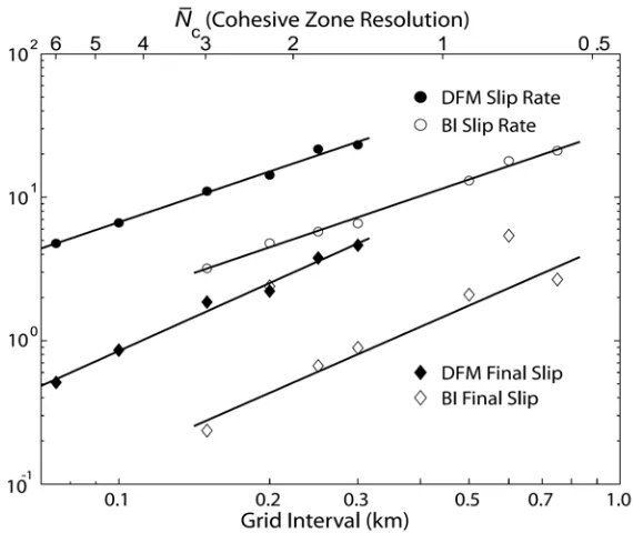
2.4 Differences in final slip (diamonds) and peak slip velocity (circles), relative to reference
solution, shown as a function of grid interval Δx . Differences are RMS averages
over the x and z axes of the fault plane. Open symbols are BI solutions, relative to
BI0.1 (the smallest grid-interval BI case). Solid symbols are DFM solutions, relative
to DFM0.05 (the smallest grid-interval DFM case). Note the power-law convergence of
both methods as the grid size is reduced. The 90% confidence intervals on the
power-law exponents suggested by the regression lines are: BI displacement [1.07–1.99]; DFM
displacement [1.31–1.84]; BI velocity [1.04–1.33]; DFM velocity [1.02–1.33]. Outliers at
Δx= 0.2 km and 0.6 km were not used in estimating the BI displacement slope. . . . 27
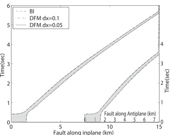
2.5 Contour plot of the rupture front for the dynamic rupture test problem. Solid curves
are for DFM0.05 (grid size Δx= 0.05 km); dotted curves are for DFM0.1 (grid size
Δx= 0.1 km); dashed curves are for BI0.1 (grid size Δx= 0.1 km). . . 28
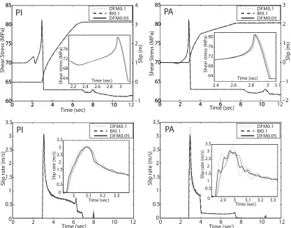
2.6 Time histories at the two fault-plane points marked in Figure 2.1. PI is on the in-plane
(x) axis, and PA is on the anti-plane (z) axis. Shear stress, slip, and slip velocity are
shown for solutions DFM0.05, DFM0.1, and BI0.1. The time histories of BI0.1 and
DFM0.05 are virtually identical, with DFM0.1 also very close. . . 30
2.7 A planar fault separating materials of different elastic properties. Some theories and
numerical simulations suggest that there is a preferred rupture propagation direction
along bimaterial fault (Weertman, 1980; Adams, 1995; Shi and Ben-Zion, 2006). . . . 35
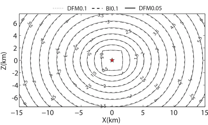
2.8 Contour plot of the rupture time on the bimaterial fault for the Southern California
Earthquake Center (SCEC) Code Validation Project Problem, Version 7. Red curves
are for BI method, and black curves are for DFM method. Contour lines are plotted
every 0.5 seconds. Rupture propagation along horizontal direction is asymmetric due
3.1 (a) A model of a planar interface embedded in an infinite and homogeneous elastic
medium. (b) A vertical strike-slip fault in an elastic half-space. The top part of the
fault is governed by rate and state friction, and the bottom part is steadily moving due
to tectonic loading.. . . 40
3.2 Properties of the simulated fault segment. (a) Rate and state friction acts on the top
24 km of the fault. A potentially seismogenic region of velocity-weakening properties
(shown in white) is surrounded by velocity-strengthening regions (shown in yellow).
Belowz =−24 km, steady motion of 32 mm/year is imposed. (b) Depth dependence
of friction parameters (a−b), a, and L in the seismogenic region. The distributions
are piecewise linear between the following points: (a−b)|z|=0 = 0.008,(a−b)|z|=4 = −0.004,(a−b)|z|=13.5=−0.004,(a−b)|z|=17.5= 0.015,(a−b)|z|=24= 0.024, a|z|=0=
0.019, a|z|=4 = 0.015, a|z|=17.5 = 0.015, a|z|=24 = 0.024, L|z|=0 = 24 mm, L|z|=4 = 8 mm,L|z|=24= 8 mm. . . 43 3.3 Long-term histories of slip and slip velocity history at two representative fault
loca-tions, P1 from the velocity-weakening region and P2 from the velocity-strengthening
region. Slip velocity is plotted on the logarithmic scale. (a),(c) Point P1 (9 km,-8 km)
exhibits stick-slip behavior. It is virtually locked for most of the time (with slip velocity
three orders of magnitude below the plate rate) but occasionally slips very fast, with
maximum slip velocity on the order of 1 m/s. (b),(d) Point P2 (-18 km,-8 km) moves
throughout the simulated time. After each dynamic event, it has postseismic slip, with
3.4 Snapshots of spatial slip-velocity distribution during a typical earthquake cycle for
L = 8 mm (h∗/Wseis = 0.8). Slip history between the 9th and 10th events is illus-trated. Colors represent slip velocity on the logarithmic scale. White and bright yellow
correspond to seismic slip rates, orange and red correspond to aseismic slip, and black
corresponds to locked portions of the fault. Each panel shows the timetof the snapshot
in years (in the upper-right corner) and the corresponding time step Δtin seconds (at
the bottom of each panel). Panels A–C also show the time in seconds elapsed since the
time of panel A. The simulations reproduce dynamic events (panels A–C and K–L),
postseismic slip (panels D–E), and the interseismic period (panel F). Aseismic transient
slip occurs between panels F and J and it is shown in panels G8–I8 of Figure 3.6 on a
different slip-velocity scale. . . 53
3.5 Snapshots of spatial slip-velocity distribution during a typical earthquake cycle for
L= 4 mm (h∗/Wseis= 0.4). Slip history between the 2nd and 3d events is illustrated. Colors and time markings have the same meaning as in Figure 3.4. Compared with
the case with L = 8 mm (Figure 3.4), dynamic events in the case with L = 4 mm
have smaller nucleation size, nucleate closer to the rheological transition (panels A,
L), have more unilateral propagation, and develop faster rupture speeds (panels A–C).
Consistent with the smaller value ofh∗/Wseis, the velocity-weakening region experiences less aseismic slip, with large portion of the region still locked when a seismic event
nucleates (panels A, J–L). Smaller aseismic transients still occur between panels F and
3.6 Snapshots of spatial slip-velocity distribution illustrating aseismic transients. White
dashed rectangles show the extent of the velocity-weakening region. Panels G8–I8
correspond to the simulation withL = 8 mm. The aseismic transient travels around
the locked portion of the fault. The average rupture speed between panels G8 and I8
is about 10 km/s and the maximum slip velocity is about 10−7m/s. The aseismic slip accumulated in the seismogenic region is equivalent to that of aMw= 5.8 earthquake.
Panels G4–I4 correspond to the simulation with L = 4 mm. The spatial extent of
the transients is smaller. Again, the transients travel around the locked portion of the
fault. Comparison of the two cases shows that the transients are confined to the band
of the velocity-weakening region next to rheological transition which experiences slow
slip in the interseismic period. The width of the band scales with the nucleation size
and its estimateh∗. That is why smaller values ofh∗/Wseis lead to smaller and more localized aseismic transients. . . 55
3.7 Slip accumulation along the linez=−8 km for the case of the homogeneous seismogenic
region. Red dashed lines illustrate fast slip; they are plotted every 2 s when maximum
slip velocity over the fault exceeds 1 mm/s. Green solid lines are plotted every 5 years,
representing slip accumulation in interseismic periods. (a) The case with L = 8 mm
settles into a periodic two-event pattern. (b) The case with L = 4 mm results in
periodic events. In the latter case, dynamic ruptures propagate faster and are more
pulse-like. In both cases, points at the nucleation zones accumulate less slip seismically
3.8 Shear stress as a function of slip during a representative dynamic event (the 9th one
in the sequence) for four locations on the fault with (a)L= 8 mm and (b) L= 4 mm.
In both cases, dynamic rupture propagates from the left side of the fault to the right
side, passing the velocity-weakening locations (-3 km, -8 km), (3 km, -8 km), (9 km,
-8 km), and then influencing the velocity-strengthening location (18 km, -8 km) as the
rupture arrests in the velocity-strengthening region. Zero slip for each point is chosen
as the slip when shear stress at the point reaches its peak during the dynamic event.
We see that the effective dependence of stress on slip is similar to linear slip-weakening
friction, with the slip-weakening rateW ≈σb/L. The velocity-strengthening point has
a smaller values of b than the other three points and hence a smaller slope. In the
case withL= 8 mm, rupture accelerates while propagating through the points shown
(Figure 3.7a), leading to different effective peak strength and slip-weakening distances
for the three velocity-weakening points. In the case withL= 4 mm, the rupture has
nearly reached its limiting speed and it is almost steady (Figure 3.7b), leading to similar
behavior of the velocity-weakening points. . . 58
3.9 Accumulation of slip along the linex= 3 km, for the fault with the homogenous
seis-mogenic region and the case ofL= 8 mm. Lines have the same meaning as in Figure
3.7. Different near-surface parameter distributions are explored. (a) In the case of
Sec-tion 3.2.1–3.2.2 and Figures 3.3–3.8 with constant normal stress and depth-dependent
L, dynamic events do not reach the free surface, arresting in the velocity-strengthening
region. The free surface accumulates large slip deficit, which is compensated by
aseis-mic slip. (b) For depth-independentL and normal stress decreasing towards the free
surface (the same distributions as in the 2D model of Lapusta et al. (2000)), dynamic
ruptures propagate all the way to the free surface, consistently with the results of
La-pusta et al. (2000). (c) When distributions of parametersaandb in the case of panel
(b) are modified to match the distributions ofσaandσb of the case in panel (a), the
3.10 Fully dynamic simulations with different cell sizes Δx. (a),(b) Slip accumulation along
the line z = −8 km for Δx = 50 m and 400 m, respectively. The results can be
compared with Figure 3.7a that shows slip accumulation for Δx = 100 m. (c)
Slip-velocity history of the fault location (9 km, −8 km) during the 5th event for Δx=
50 m, 100 m, 200 m, and 400 m. Zero in time corresponds to rupture arrival at the
location (6 km, −8 km). The values Δx = 50 m and 100 m are both several times
smaller than the quasi-static cohesive zone size Λ0 = 300 m and produce
resolution-independent results. Δx= 200 m provides less adequate resolution and Δx= 400 m
leads to very different results. The numerical resolution in our simulations is dictated
by the cohesive zone size, as the nucleation sizeh∗, another important length scale, is several times larger. . . 59
3.11 Fully dynamic simulations with different values of the truncation parameterα. (a),(b)
Slip accumulation along the line z = −8 km for α = 2 and 1/3, respectively. The
results can be compared with Figure 3.7a that shows slip accumulation for α= 3/2.
(c) Slip-velocity history of the fault location (12 km,−8 km) during the 5th event for
α= 1/3, 1/2, 3/2, 1, and 2. Zero in time corresponds to rupture arrival at the location
(6 km, −8 km). Larger values of α lead to inclusion of longer slip histories in the
dynamic response calculation. α= 2,3/2, and 1 produce similar results, whileα= 1/2
and 1/3 cause differences as discussed in the text. . . 60
3.12 Slip-velocity history of the fault location (12 km,−8 km) during the first event in fully
dynamic simulations with different values of the truncation parameterρc. Zero in time
corresponds to the rupture arrival at the location (3 km, −8 km). Larger values of
ρc make the frequency-dependent truncation closer to the frequency-independent one.
Our frequency-dependent truncation withρc= 3π/2 approximately corresponds to the
truncation parameters in Lapusta et al. (2000). ρc≥100 produce the same results as
3.13 Snapshots of slip-velocity distribution during the first (top row) and second (bottom
row) events for the case with a stronger patch. The slip-velocity range shown is different
from Figures 3.4–3.6 and chosen to emphasize the rupture front. The number in the
upper-right corner of each snapshot indicates the elapsed time (in seconds) since the
first snapshot for each event. During the first event, dynamic rupture interacts with
the stronger patch and produces a supershear burst. During the second event, no
interaction or supershear propagation occurs; the stronger patch is indicated by a red
circle in this case. Rupture behavior of the first event does not repeat in the slip history
of the fault due to redistribution of shear stress. . . 63
3.14 Distribution of shear stress along the linez =−8 km during the 1st and 2nd events,
at the time when the horizontal rupture front (at this depth) arrives approximately
at the center of the fault (x = 0 km). In the 1st event, the patch has similar shear
stressτ as the surrounding area but 20% larger normal stressσ, resulting in smaller
nondimensional prestressτ /σ than the rest of the fault. However, in the second event,
τ inside the patch is about 20% larger than in the surrounding area, resulting in
homogeneous nondimensional prestressτ /σ. This redistribution of shear stress due to
prior slip history eliminates the interaction of dynamic rupture with the patch observed
in the first event. . . 65
3.15 Snapshots of slip velocity during the first three events forσh = 1.4σ, 1.6σ, and 2.0σ.
Black circles are plotted to indicate the location of the heterogeneity. Due to
redistri-bution of shear stress with slip, the interaction of dynamic rupture with heterogeneity
becomes insignificant after the first three events. . . 67
3.16 Earthquake recurrence periodTfor different heterogeneity strengthsσh. Higher normal
stress inside the patch increases the shear stress drop in dynamic events, and thus
tends to increaseT. On the other hand, higher normal stress decreases the earthquake
3.17 Accumulation of slip along the linez=−8 km for the case with a stronger patch. Lines
have the same meaning as in Figure 3.7. (a) Results for the fully dynamic simulation.
The slip pattern of the fault with a small stronger patch (which occupies less than 1%
of the seismogenic area) is different from the one with the homogeneous seismogenic
region (Figure 3.7a). (b) The standard quasi-dynamic formulation (βs= 1) results in
a modified slip pattern, smaller slip velocity, slower rupture speeds, and smaller slip
per event. (c),(d) Larger values of βs = 1 or smaller radiation terms in the
quasi-dynamic formulation accelerate rupture speed and increase slip velocity. However, all
quasi-dynamic simulations produce similar slip patterns that are qualitatively different
from the fully-dynamic one. . . 69
3.18 Comparison of fully dynamic and quasi-dynamic simulations of one dynamic event
(the first event in the sequence). (a),(b) Slip-velocity and slip histories of the fault
location (9 km, -8 km). Zero time corresponds to the time of rupture arrival at the
point (6 km, -8 km). Slip velocity and slip per event in quasi-dynamic simulations is
significantly smaller than in the fully-dynamic one. Simulations with largerβsproduce
faster rupture speeds, larger slip velocity, and larger slip per event. However, when
scaled appropriately, the quasi-dynamic results all collapse onto the same curves (insets
in panels (a) and (b)). (c),(d) Rupture speed as a function of rupture tip location
along z = −8 km. The quasi-dynamic simulation with βs = 4 has larger rupture
speeds than the fully-dynamic simulation. All quasi-dynamic simulations have nearly
3.19 Cohesive zones in quasi-dynamic simulations. (a) Shear stress distribution along the
horizontal linez=−8 km at the time of rupture front arrival at point (−7.9 km, −8
km) during the first event in the simulation withβs= 1. Crosses indicate locations of
spatial cells (Δx= 50 m). The rupture speed at that time is 0.12 km/s. The cohesive
zone size is 0.3 km. The bottom panel shows the accumulation of slip in that case,
with the double arrow indicating the distance plotted in the main panel. (b) Shear
stress distribution along the horizontal line z = −8 km at the time of rupture front
arrival at (0.24 km,−8 km) km during the first event in the simulation with βs = 4.
The rupture speed at that time is 2.45 km/s. Despite the different value of βs and
the different rupture speed, the cohesive zone size is still 0.3 km. In quasi-dynamic
simulations, the cohesive zone size does not shrink during rupture propagation and its
size is independent of the parameterβs. . . 72
3.20 Elastodynamic kernelsKIII(ρ) and KII(ρ). (a),(b) Values of the kernels for relatively
small kernel arguments. (c),(d) Comparison of kernels with the leading terms in their
asymptotic expansions. Forρ1,KIII(ρ)∼O(ρ−3/2) andKII(ρ)∼O(ρ−1/2). KII(ρ) decays much slower thanKII(ρ) asρincreases. . . 75
4.1 (a) Linear slip-weakening friction law. τc is the shear strength of the interface and δ
is slip (or relative displacement in shear) across the interface. (b) A prescribed crack
interface is embedded in an infinite, elastic, and homogeneous space. The main crack
is initiated from a region aroundx= 0. This work considers interaction of the main
crack with a region of heterogeneity that exists in front of the main crack and may
initiate a secondary crack. Depending on the model, the heterogeneity is a pre-existing
subcritical crack, a patch with higher prestress, or a patch with lower peak friction
strength. When discussing crack tips and their speeds for both main and secondary
cracks, we always refer to crack tips that propagate in the direction of increasingx, or
4.2 (a) Shear stress distribution for a mode II crack spontaneously propagating on an
interface governed by linear slip-weakening friction. A peak in shear stress travels
with the shear wave speed in front of the crack. The interface has uniform friction
properties and uniform prestressτogiven by (τo−τd)/(τs−τd) = 0.53. (b) Rupture
time along the interface, i.e., the time at which each point along the interface first
acquires nonzero speeds. A daughter crack appears in front of the main crack at
the location x/Lc = 13.5 and propagates with intersonic speeds as described by the
Burridge-Andrews mechanism. Here and in the text the word “intersonic” refers to
speeds between the shear wave speedcsand the dilatational wave speedcp. For lower
prestress, the daughter crack would appear further along the interface or not at all. . 83
4.3 Stress distribution on the interface for different initiation procedures. To compare
stress fields created by the main crack, no heterogeneity at ¯x= 12 is imposed for these
simulations. The more abrupt initiation procedure that results in a higher shear stress
peak is discussed in Section 4.4. . . 88
4.4 Stress distribution around the main crack and pre-existing subcritical crack at ¯t = 0
(solid green line). The main crack centered at ¯x= 0 is poised to propagate
sponta-neously fort >0, while the secondary crack centered atx= 12Lcremains a subcritical
crack. Prestress outside of zones affected by cracks is equal to ¯τo = 0.33. ¯τBA = 0.53
(black dashed line) is the prestress level required for intersonic transition at the location
¯
4.5 Left panel: Rupture time along the interface for the case with a preexisting subcritical
crack. Under the stress field of the advancing main crack, the secondary subcritical
crack begins to spread at ¯t=cst/Lc = 7.9 and eventually propagates with intersonic
speeds. Note that the results of simulations with two resolutions,Nc= 200, β= 4 and
Nc= 1200, β= 4, are almost indistinguishable on the scale of the plot. More resolution
comparisons are shown in Figure 4.6. Right panel: Rupture speed of the secondary
crack. It approaches the Rayleigh-wave speed and then abruptly jumps to intersonic
speeds. Rupture speed is determined for the case with resolutionNc= 1200, β= 4 by
dividing the interface into intervals of 24 cells each, computing average rupture speed
over each interval, and plotting the obtained value with respect to the middle of the
interval. Care is taken to make the location of the rupture speed jump correspond to
a beginning or end of an interval.. . . 89
4.6 Propagation of the secondary crack in the region where sub-Rayleigh-to-intersonic
tran-sition occurs. Rupture time of each spatial cell is indicated using different symbols for
different resolution. For progressively finer resolution (i.e., larger Nc), transition
oc-curs within one cell size Δxand one time step Δt, which means that, in the limit of
Δx→0 and Δt→0, the rupture front abruptly jumps from speeds numerically equal
tocR= 0.92csto an intersonic speed. . . 90
4.7 Snapshots of slip velocity (left) and shear stress distributions (right) on the interface
during sub-Rayleigh-to-intersonic transition for the case Nc = 1200, β = 4, zooming
in on the crack tip. Slip velocity is plotted on the logarithmic scale. For plotting
convenience, slip velocity shown is the actual slip velocity plus 10−6 and hence zero slip velocity appears as 10−6 on the plot. At time ¯t =cst/Lc = 15.02, the crack tip propagates with the speed numerically equal tocR. At ¯t= 15.04, sliding initiates just
4.8 Shear stress distribution around the main crack (left panel) and the patch of higher
prestress (right panel) at ¯t = 0 (¯τo = 0.33). In the left panel, the solid green and
dashed red lines correspond to the smooth and more abrupt initiation procedures,
respectively. ¯τBA= 0.53 is the level of prestress required to achieve Burridge-Andrews
intersonic transition at the location ¯x= 13.5 with the smooth initiation procedure. . . 92
4.9 Influence of patch parameters on eventual intersonic vs. sub-Rayleigh propagation for
three different values of background prestress and more abrupt initiation of the main
crack. The horizontal and vertical axes indicate the patch prestress and patch size,
respectively. Red filled dots indicate simulated cases for which rupture has sustained
intersonic speeds beyond the higher-stressed patch. Black open dots indicate simulated
cases for which rupture stays sub-Rayleigh. Dashed green lines indicate approximate
boundaries of different behavior. The valueαof the patch prestress is discussed in the
text. . . 94
4.10 Influence of patch parameters on intersonic vs. sub-Rayleigh propagation for smooth
initiation of the main crack that results in a smaller shear stress peak. The horizontal
and vertical axes indicate the patch prestress and patch size, respectively. Red filled
dots indicate simulated cases for which rupture has sustained intersonic speeds beyond
the higher-stressed patch. Black open dots indicate simulated cases for which rupture
stays sub-Rayleigh. Dashed green lines indicate approximate boundaries of different
behavior. The valueαof the patch prestress, blue star, and two cases marked by small
4.11 Rupture time for different patch sizes, with ¯τo = 0.25 (S = 3) and more abrupt
initiation of the main crack. Left panel: Patch prestress ¯τo
h= 0.85. Rupture eventually propagates with intersonic speeds for ¯Lh=Lh/Lc= 0.075 and 0.34 and sub-Rayleigh
speeds for ¯Lh= 0.055 and 0.20. Behavior for these and other patch sizes is discussed
in the text. Right panel: Patch prestress ¯τo
h = 0.70, note a different scale of ¯x. The behavior is much simpler than for ¯τho = 0.85. Cases with different ¯Lh are marked by
letters A–E at the location ¯x= 12 + 2 ¯Lhwhere the secondary crack for each case leaves
the patch. ¯Lh= 0.08, line A: the secondary crack is overtaken by the main crack for
this and smaller ¯Lh. ¯Lh= 0.1,0.105,0.11,0.115,0.12, line B: for 0.1≤Lh¯ ≤0.115, the
secondary crack accelerates to cR and abruptly transitions to intersonic speeds, but
reverts back to sub-Rayleigh speeds after short (but progressively longer) intersonic
propagation; for ¯Lh= 0.12, the crack manages to stay intersonic and results in eventual
intersonic propagation. Lh¯ = 0.20,0.30,0.45, lines C, D, E: same behavior as for ¯
Lh= 0.12 . . . 98
4.12 Snapshots of stress and slip velocity for the cases of ¯Lh= 0.075 (solid green line) and ¯
Lh= 0.20 (black dashed line with smaller dashes) with ¯τo= 0.25, ¯τo
h = 0.85, and more abrupt initiation of the main crack. Propagation of the main crack with no patch of
higher prestress is also shown (red dashed line with larger dashes). . . 100
4.13 Left: G(1/vr,1/c) = (˜τ(c)−τo)/(τo−τd) for differentc > cs and rupture speed vr.
Right: Mode II kernelM(u) of the space-time representation off(x, t). . . 109
5.1 (a) A buried strike-slip fault model which is 180 km long and 36 km wide. The region
where friction acts is Lfric = 120 km long and Wfric = 24 km wide. It is separated
into a potentially seismogenic velocity-weakening region (white color, Lseis = 60 km,
Wfric= 10 km), and a velocity-strengthening region (yellow color). The outside region
moves with the constant loading rateVpl= 10−9 m/s = 32 mm/year. Figure (b) and (c) show distributions of friction parameters a and b along horizontal line z = 0 km
5.2 Distribution of shear stress at the beginning of each simulation along z = 0 km (left
panel) andx= 0 km (right panel) . . . 118
5.3 Typical behavior of a location within the seismogenic region, with (0 km, 0 km) used
as an example. (a)–(c) Shear stress vs. slip, shear stress vs. time, slip vs. time for
Case I. Zero time is the starting time of the third event, and slip is set to be zero at
the zero time. Seismic ratio at this location is 2.08 > Scrit,3D(= 1.19) in this event.
Nonetheless, rupture passes this location with an intersonic speed. τp, τi, τd, and τe
are defined in the text. (d) Shear stress vs. slip for Case II. Zero time is the starting
time of the third event. Seismic ratio is 2.21, and rupture passes this location with a
subsonic speed. For both Cases I and II,Vdynis of the order of 1 m/s, andT is of the
order of 100 years. Largeraresults in higher seismic ratio S in Case II, making Case
II less susceptible to intersonic propagation. . . 121
5.4 (a) Slip accumulation along the horizontal linez = 0 km in Case I. Red dashed lines
are plotted every 1 second when maximum slip velocity on the fault exceeds 1 mm/s,
representing slip accumulation during seismic periods, and green solid lines are plotted
every 5 years, representing slip accumulation in aseismic periods. The 1st, 3rd, 5th
and 9th events have global intersonic propagation. (b) Maximum slip velocity on the
5.5 Snapshots of slip velocity in the third and sixth events for Case I. Slip velocity is shown
on the logarithmic scale, ranging from 10−12 m/s to 1 m/s. White and bright yellow correspond to seismic slip velocity, and black corresponds to locked portions of the
fault. The white dashed boxes in the top panels indicate the location of the
velocity-weakening region. Zero time is the starting time of each event. The time interval
between two successive panels is 2.22 s. The blue dashed line is plotted to indicate the
position of the rupture front (at depthz= 0 km) if it propagates with the shear wave
speed of 3 km/s. The two events have similar initial rupture propagation (before the
time of 7.78 s), but afterwards the third event propagates appreciably faster than the
sixth event. . . 124
5.6 (a) and (b): Rupture time of the third and sixth events for Case I; (c) and (d):
Hori-zontal rupture speedc(x, z) for the same events. . . 125
5.7 (a) Rupture speedc∗(x) as a function of strike distancexfor the third and sixth events in Case I. The third event has global intersonic propagation, but the sixth event does
not. (b) Average slip ¯δ(x) as a function of strike distance x for the third and sixth
events in Case I . . . 127
5.8 Distribution of initial shear stress τi for the third (intersonic) and sixth (subsonic)
events of Case I . . . 127
5.9 (a) Interseismic slip accumulation along central vertical line x = 0 km between the
second and third events of Case I (red dashed line) and slip distribution assumed in a
2D anti-plane model (blue solid line). (b) The corresponding shear stress accumulation 129
5.10 Distribution of seismic ratio S = (τp −τi)/(τi −τd) on the fault (within
velocity-weakening seismogenic region) for the third and sixth event of Case I . . . 130
5.11 (a) Slip accumulation along the horizontal linez= 0 km in Case II, with a homogeneous
velocity-weakening region. All events after the first one are subsonic. (b) Maximum
5.12 Snapshots of slip velocity on the fault for the third event of Cases II and IIh1. The blue
line is plotted to indicate the shear wave speedcsof 3 km/s. A weaker patch of lower
peak resistance in Case IIh1 makes the entire rupture transition to intersonic speeds.. 132
5.13 (a) Fault model of Case IIh1: a buried strike-slip fault model with a weaker patch
(red) centered at (-5 km, 0 km). Figure (b) and (c) show the distributions of friction
parametersaandbalong horizontal linez= 0 km and vertical linex= 0 km in Cases
IIh1 and IIh2, respectively. In Case IIh2, the heterogeneity is of the same size as in
Case IIh1 but centered at (5 km, 0 km). . . 133
5.14 (a) Slip accumulation along the horizontal linez = 0 km in Case IIh1. (b) Maximum
slip velocity in logarithmic scale vs. time in unit of years . . . 134
5.15 (a) Slip accumulation along the horizontal linez = 0 km in Case IIIb. (b) Maximum
slip velocity in logarithmic scale vs. time in unit of years . . . 134
5.16 Figure (a), (b), and (c): rupture time of the third event for Case II, IIh1, and IIh2,
respectively; Figure (c), (d), and (e): horizontal rupture speed c(x, z) on the fault
of the third event for Case II, IIh1, and IIh2, respectively. The black dashed boxes
in Figures (e) and (f) indicate the locations of the weaker patch. Global intersonic
transition occurs in Case IIh1 and IIh2, and the transition occurs approximately at the
location of the weaker patch. . . 136
5.17 Distribution of seismic ratio S = (τp −τi)/(τi −τd) on the fault (within
velocity-weakening seismogenic region) of the third event for Cases II, IIh1, and IIh2,
respec-tively. Due to low seismic ratio in the patch in Case IIh1 and IIh2, secondary cracks
are initiated there in front of the main rupture, and driven to intersonic speeds by the
5.18 Initiation of an intersonic secondary rupture in the third event of Case IIh1. (a)–(c):
Snapshots of shear stress distribution along the strike distance atz= 4 km depth, next
to a rheological boundary, at the timest= 6.1 s, 7.1 s, and 8.1 s, respectively. (d)–(f):
Corresponding snapshots of slip velocity. Red solid lines represent the location of the
weaker patch. Blue dashed lines represent the horizontal locations of shear stress peak.
The secondary rupture initiates in the weaker patch ahead of the shear stress peak,
consistent with our findings in Chapter 4. . . 139
5.19 (a) Average shear stress ¯τi before each event in Case I. (b) Effective seismic ratio ¯S for
each event in Case I. Red solid dots represent intersonic events and blue empty circles
represent subsonic events. . . 140
5.20 Effective seismic ratio ¯S and average initial shear stress ¯τi before each dynamic event
for Cases II, IIh1, and IIh2. Red solid dots represent intersonic events and blue empty
circles represent subsonic events. . . 141
5.21 Distribution of stress drop Δτ =τi−τe for the third and sixth events of Case I. The
distribution is heterogeneous due to the presence of rheological boundaries. . . 144
5.22 Distribution of final slip δe(x, z) on the fault due to the third (intersonic) and sixth
(subsonic) events for Case I. In each panel, the red star indicates the event hypocenter.146
5.23 Rupture time along the linez=−4 km in the third event of Case IIh1. The black solid
line is the original rupture timetr, and the red dashed line is the adjusted rupture time
List of Tables
2.1 Stress and frictional parameters for test problem . . . 16
2.2 Test problem calculations . . . 17
3.1 Parameters of our simulations. For depth-dependent quantities marked with the
aster-isk “∗”, the typical value over the velocity-weakening (potentially seismogenic) region is specified. . . 56
4.1 Values of S, Lnucl/Lc, and numerical resolution of Lc and Λo for different prestress
levels τo. Nc = 100 is the lowest resolution used. Numerical convergence has been
verified by consideringNc equal to 200, 400, and, in some cases, 1200, which increases
the resolution of the cohesive zone by a factor of two, four, and twelve, respectively. . 86
5.1 Case-independent parameters . . . 117
5.2 Case-dependent parameters . . . 117
Chapter 1
Introduction
Frictional interfaces respond to loading with both stick-slip behavior and steady sliding. An example of considerable practical importance is the relative displacement or slip on faults in the Earth’s crust. Driven by slow tectonic motion equivalent to centimeters of slip per year, fault processes involve both seismic events or earthquakes and complex patterns of quasi-static aseismic slip (Figure1.1). Understanding the physics and mechanics of this behavior is a fascinating scientific problem. In this thesis, we first develop computational tools for three-dimensional (3D) modeling of dynamic rupture and long-term fault slip. Then the tools are applied to the fundamentally and practically important phenomenon of intersonic transition and propagation of dynamic rupture.
wave propagation through elastic media, because that wave propagation is accounted for through the convolutions. The challenge is then to determine the appropriate convolution kernels, which is possible to do analytically only for relatively simple situations such as crack propagation in an infinite, uniform elastic solid. It may be possible to consider more complex problems (such as a layered elastic medium) by precalculating convolution kernels numerically as briefly discussed in
Lapusta et al. (2000), but to our knowledge this has not yet been implemented. This makes BI methods more restrictive than finite-element or finite-difference methods. However, BI methods are more efficient (Chapter 2) and allow extensions to simulations of long-term deformation histories punctured by rapid dynamic events (Lapusta et al., 2000, Chapter3).
Since spontaneous rupture problems are highly nonlinear and do not have analytical solutions, it is necessary to compare our implementation of the boundary integral methodology and finite difference algorithms. The nonlinearity is attributable to the fact that rupture evolution and arrest are not specified a priori, and they are determined as part of the problem solution. That is, the problem is a mixed-boundary value problem in which the respective (time-dependent) domains of the kinematic and dynamic boundary conditions have to be determined as part of the problem solution itself. In the absence of a strict mathematical proof that either method converges to an exact solution for spontaneous rupture problems, the comparison provides validation for both numerical approaches, because these numerical methods have a high degree of independence. The boundary integral method may be called a semi-analytical method, because it discretizes only the fault surface points; the reaction of the continuum to slip at those points is represented exactly, through a closed-form Green’s function. In contrast, the finite difference method uses a volume discretization to approximate the differential equations of motion throughout the 3D problem domain.
challenging because of the variety of temporal and spatial scales involved. Slow loading requires hundreds to thousands of years in simulated time and fault zone dimensions are in tens to hundreds of kilometers. At the same time, rapid changes in stress and slip rate at the propagating dynamic rupture tip occur over distances on the order of meters and times on the order of a small fraction of a second.
Several approaches to modeling long-term histories of fault slip have been proposed (e.g.,Shibazaki and Mastsu’ura,1992;Cochard and Madariaga,1996;Kato,2004;Duan and Oglesby,2005;Liu and Rice, 2005;Hillers et al.,2006;Ziv and Cochard,2006;Aagaard and Heaton,2008) but all of them adopted simplified treatments of either slow tectonic loading and hence aseismic slip, or inertial effects during dynamic rupture, or transition between interseismic periods and dynamic rupture.
Lapusta et al. (2000), based on prior studies (Tse and Rice,1986;Rice and Ben-Zion, 1996; Ben-Zion and Rice,1997), developed a methodology capable of capturing both seismic and aseismic slip and the gradual process of earthquake nucleation. However, the model of Lapusta et al. (2000) is two-dimensional (2D) and neglects variations in the along-strike fault dimension. Therefore it cannot be directly compared to observations and cannot be used to study a number of important problems such as interaction of fault slip with compact fault heterogeneities. In 2D models, the fault is simplified to a line, and any heterogeneity in stress or friction properties blocks the entire fault. In 3D models, the fault is represented as a surface that can include local heterogeneities and complex patterns of frictional and other properties.
Figure 1.1: An example of interaction between earthquakes and aseismic quasi-static slip. Earth-quakes redistribute stress on faults, causing slow postseismic slip or afterslip in surrounding areas, as shown here on the example of 2005 Nias-Simeulue earthquake in Sumatra (fromHsu et al.,2006). The postseismic slip, in turn, redistributes stress and may trigger other seismic events. The figure shows compilation of inferred seismic and postseismic slip, illustrating the approximately compli-mentary nature of seismogenic and aseismic regions. Distribution of seismic slip is indicated by white contours at intervals of 2 m; color indicates cumulative postseismic slip during the 9 months after the earthquake. Black and red vectors indicate GPS observations and their match using the inferred postseismic slip, respectively. White and red stars are epicenters of 2004 Aceh-Andaman and 2005 Nias-Simeulue earthquakes, respectively. Pink and green dots denote earthquakes with body wave magnitudemb >4.5 before and after the 2005 event. The regions of high seismicity correspond to
a range of seismic and aseismic phenomena. The model is used to explore the effect of several physical and numerical parameters.
We then consider two application examples that demonstrate (i) the importance of conducting long-term simulations even if the main emphasis is on the behavior of dynamic rupture and (ii) the necessity of including inertial effects in long-term simulations of slip. In the first example, we study how fault slip interacts with compact heterogeneity in the form of a patch of higher normal stress over many earthquake cycles. This kind of problem cannot be addressed with a 2D fault model. Such patches can result on natural faults from slight local non-planarity of the fault surface. 3D simulations of single dynamic events suggest that such fault heterogeneities can strongly influence the development of dynamic ruptures, in part, inducing intersonic rupture speeds (e.g., Dunham et al., 2003). However, in simulations of single dynamic events, specified initial conditions, such as initial shear stress, have a determining effect on the resulting dynamic rupture. Our methodology for earthquake cycle modeling allows us to simulate the interaction of slip with heterogeneity under conditions that naturally develop in the model due to prior seismic and aseismic slip, and to compare that evolved behavior with the one due to arbitrarily chosen initial conditions. We do find significant differences between dynamic rupture behavior in the first and subsequent events, demonstrating the importance of simulating long-term slip histories. In the second example, the fully dynamic formulation developed in this work is compared with quasi-dynamic approaches, which have been widely used in earthquake studies (e.g.,Rice,1993;Cochard and Madariaga,1994;
Ben-Zion and Rice, 1995; Rice and Ben-Zion, 1996; Hori et al., 2004; Kato, 2004; Hillers et al.,
2006; Ziv and Cochard, 2006). Quasi-dynamic approaches significantly simplify the treatment of inertial effects during simulated earthquakes by ignoring wave-mediated stress transfers. Results of our comparison underscore the importance of including full inertial effects. We also explore the possibility of improving the standard quasi-dynamic formulation by decreasing the radiation damping term, as suggested byLapusta et al.(2000).
5.3 km/s
Figure 1.2: An example of inferred intersonic propagation in a large strike-slip earthquake. The 2002 Denali (Alaska) earthquake produced a surface rupture of about 340 km (dark blue line). Modeling of near-fault acceleometer records suggests that the rupture in a segment of about 40 km (red line) may have propagated with intersonic speeds, with an average speed of 5.3 km/s (Ellsworth et al.,2004).
problem in fracture mechanics with important practical implications for earthquake dynamics and seismic radiation. The word “intersonic” refers to speeds between the shear wave speedcs and the
dilatational wave speedcp, the range which is often called “supershea” in the geophysical literature.
Although average rupture speeds for earthquakes are often subsonic in general, seismic data for several earthquakes points to intersonic propagation. Examples are 1979 Imperial Valley earthquake (Archuleta,1984;Spudich and Cranswick,1984), 1992 Landers earthquake (Olsen et al.,1997), 1999 Izmit earthquake (Bouchon et al.,2001), 2001 Kunlun earthquake (Bouchon and Vall´ee,2003), and 2002 Denali earthquake (Ellsworth et al.,2004, Figure1.2). While this evidence is indirect, as it is obtained through analysis of seismic data, it presents a compelling case that intersonic propagation and hence sub-Rayleigh-to- intersonic rupture transition can occur during earthquakes.
speed histories. Xia et al.(2004) reported experimental observations of spontaneous sub-Rayleigh-to-intersonic transition of mode II cracks propagating along a frictionally held homogeneous interface.
Xia et al.(2005) experimentally observed a change in rupture speed from sub-Rayleigh to intersonic along a bimaterial interface.
Studies of sub-Rayleigh-to-intersonic transition have important practical implications. On the one hand, understanding which parameters and conditions do, and do not, lead to intersonic rupture propagation in models can help constrain properties and stress conditions on natural faults where rupture speeds of large earthquakes have been inferred. On the other hand, it is important to know which conditions can lead to intersonic propagation on faults and how likely intersonic ruptures are to occur. This is because intersonic ruptures can cause much stronger shaking far from the fault than subsonic ruptures can, as Mach fronts generated by intersonic ruptures carry large stresses and particle velocities far from the fault (Bernard and Baumont, 2005; Dunham and Archuleta, 2005;
Bhat et al., 2007).
Theoretical and numerical studies of sub-Rayleigh-to-intersonic transition date back toBurridge
(1973) and Andrews (1976). Large strike-slip earthquakes are dominated by in-plane sliding and some of their dynamics can be understood by considering them as mode II cracks. Burridge(1973) considered a self-similar mode II crack and found that a shear stress peak propagates with the shear wave speedcsin front of the crack.Andrews(1976) performed numerical simulations of spontaneous
crack propagation on a uniformly prestressed interface governed by a linear slip-weakening law, and demonstrated that a growing shear stress peak nucleates a daughter crack in front of the main rupture. The daughter crack propagates with intersonic speeds from its very beginning. This processes of intersonic transition is often called the Burridge-Andrews mechanism. Since the work of
Burridge(1973) andAndrews(1976), a number of theoretical and numerical studies have addressed the issue of sub-Rayleigh-to-intersonic transition and/or intersonic propagation, as discussed in Chapter4.
transition occurs in a number of models where a crack is subjected to an intersonic loading stress field. The Burridge-Andrews mechanism falls under that category, as a daughter crack initiates at the location of the shear stress peak and finds itself under the influence of the stress field of the advancing main crack. The stress field creates intersonic loading in front of the shear stress peak. We consider interaction of an advancing mode II crack (main crack) with a location susceptible to nucleation of a secondary dynamic crack, such as a pre-existing subcritical crack, a patch of higher prestress, or a patch of lower peak friction strength. Such locations are called collectively by “favorable heterogeneity” in this thesis. For a range of parameters, a secondary dynamic crack initiates at the location before the shear stress peak arrives, acquires intersonic speeds, and maintains intersonic propagation for large distances. We call the crack secondary to reserve the term “daughter” for cracks that initiate at the location of the shear stress peak in front of the main crack in the absence of pre-existing heterogeneity. Our results show, in part, that nucleating a daughter crack at the shear wave peak, a feature that propagates with the shear wave speed, is not essential for the subsequent intersonic propagation of the daughter crack. In our models, intersonic rupture transition can be achieved and subsequent intersonic crack propagation can be maintained under background prestress levels that are lower than the ones predicted by the Burridge-Andrews mechanism, and transition lengths depend on the position of favorable heterogeneities. Observations of transition lengths in earthquakes are sometimes interpreted using the Burridge-Andrews mechanism to infer parameters of fault friction (e.g.,Xia et al.,2004). If intersonic transition is governed by presence of heterogeneities as presented in Chapter4, such inferences may be misleading.
The results of Chapter 4 suggest that heterogeneity can have significant effect on intersonic transition and propagation. However, the 2D in-plane model of Chapter 4 contains a number of simplifications that can affect its applicability to natural earthquakes. First, Chapter4 considers 2D models of in-plane sliding to make comparison with earlier studies (Burridge, 1973; Andrews,
by 3D aspects, especially the finite fault width, which have been shown to have adverse effects on intersonic transition (Day,1982a;Madariaga and Olsen,2000;Fukuyama and Olsen,2002;Dunham,
2006). Second, stress and strength distributions on faults in the Earth’s crust can be much more complicated than assumed in Chapter4. Certain types of heterogeneous stress distributions result in slower rupture speeds than the speeds that would correspond to mean values of stress (Day,1982b). While one can assume any prestress distribution for a simulation of one instance of dynamic rupture, stress distribution on faults before a large earthquake is the result of a complicated history of seismic and aseismic sliding. That history would tend to redistribute stress and may exclude some prestress distributions before a large earthquake and hence certain rupture behaviors, as demonstrated in Chapter3. Hence it is important to simulate long deformation histories of faults, to be able to study simulated earthquakes and intersonic transition under prestress distributions that naturally arise as the result of prior sliding history. Third, we find that the initiation procedure of the main crack significantly affects intersonic transition at the heterogeneity and subsequent propagation. Hence it is important to consider ruptures nucleating in a realistic model under slow tectonic loading.
We remove these simplifications in Chapter5 by using the methodology developed in Chapter
continuing “creep-in” of the stable slip into the locked region, creating areas of high fault stress. Once earthquake rupture nucleates, it propagates faster over these areas of higher stress than over the rest of the seismogenic region, transitioning to intersonic speeds in some cases. The occurrence of intersonic transition in our 3D model depends on the combination of friction properties and fault stress that develops in the model before large earthquakes. It can be explained by considering the seismic ratio (Andrews, 1976) on the fault before large events, as discussed in Chapter 5. Since the presence of rheological boundaries on natural faults can be inferred from laboratory studies and fault observations (e.g.,Blanpied et al., 1991;Marone et al.,1991;Blanpied et al.,1995;Ellsworth et al.,2000; Marone, 1998;Lyons and Sandwell, 2002;Schaff et al.,2002;Waldhauser et al., 2004;
Shearer et al., 2005) as further discussed in Chapter 5, this factor can significantly contribute to intersonic transition on natural faults.
We then consider whether intersonic transition in 3D models of long-term slip can be further promoted by favorable compact fault heterogeneity, as suggested by the 2D single-event study of Chapter 4. We find a parameter regime in which there is no intersonic transition in the long-term history of the 3D fault model without the compact heterogeneity, and then we add a patch of lower effective peak frictional resistance to the model. Our simulations show that adding such a patch indeed qualitatively modifies the behavior of the model, resulting in occasional intersonic earthquakes. The transition distance is determined by the location of the patch, consistently with conclusions in Chapter4.
rheological boundaries parallel to the direction of rupture propagation.
Chapter 2
Modeling 3D spontaneous rupture
with boundary integral method
In this chapter, we develop a 3D spectral boundary integral algorithm to simulate spontaneous rupture and assess its accuracy and efficiency by comparing simulated results with a finite difference method (Day,1982b;Dalguer and Day,2004). This comparison is necessary as spontaneous rupture problems are highly nonlinear and do not have analytic solutions. This comparison also provides useful data for testing new numerical methods. At the end of this chapter, we expand the algorithm to simulate spontaneous rupture on the fault separating solids with different elastic properties.
Sections2.1–2.7are based on Day, Dalguer, Lapusta and Liu(2005).
2.1
Problem formulation
We consider a problem of a planar surface Σ embedded in an isotropic, linearly elastic infinite space. The linearized equations of motion for the space are
σ = μ
c2p
c2 s
−2
( ·u)I+μ( u+u ), (2.1)
¨
u = c
2 s
where σ is the stress tensor,u is the displacement vector, cs andcp are the S and P wave speeds,
respectively,μis the shear modulus, and Iis the identity tensor.
The surface Σ has a (continuous) unit normal vector n. A discontinuity in the displacement vector is permitted across the interface Σ. On Σ we define limiting values of the displacement vector,u+ andu−, by
u±(x, t) = lim
ε→0u(x±εn, t). (2.3)
We denote the discontinuity of the vector of tangential displacement (slip) byδ ≡ (I−nn)· (u+−u−) , its time derivative (slip rate) byδ˙, and their magnitudes byδand ˙δ, respectively. The
traction vectorσ·nis continuous across Σ. The shear traction vectorτ is given by (I−nn)·σ·n
with the magnitudeτ, bounded by a non-negative frictional strengthτc.
We formulate the jump conditions at the interface as follows:
τc−τ≥0, (2.4)
τcδ˙−τδ˙= 0. (2.5)
Equation (2.4) stipulates that the shear traction be bounded by the (current value of) frictional strength, and equation (2.5) stipulates that any nonzero velocity discontinuity be opposed by an antiparallel traction (i.e., the negative side exerts traction−τ on the positive side) with magnitude equal to the frictional strength τc. But note that (2.5) has been written in a form such that it remains valid when ˙δis zero. In fact, when equality does not pertain in (2.4), (2.5) can be satisfied only with ˙δequal to zero.
The frictional strength evolves according to some constitutive functional which may in principle depend upon the history of the velocity discontinuity, and any number of other mechanical or thermal quantities, but is here simplified to the well-known slip-weakening form, introduced by Ida(1972) and Palmer and Rice(1973) by analogy to cohesive zone models of tensile fracture. In that form,
coefficient of frictionf(l) that depends on the slip path length lgiven by0tδ˙(t)dt,
τc =−σnf(l). (2.6)
For this comparison, we use the linear slip-weakening friction (the same as in Chapter 4), where
f(l) is given by:
f(l) =
⎧ ⎪ ⎪ ⎨ ⎪ ⎪ ⎩
fs−(fs−fd)l/d0, l < d0;
fd, l≥d0;
(2.7)
where fs and fd are coefficients of static and dynamic friction, respectively, and d0 is the critical
slip-weakening distance (e.g.,Ida,1972;Andrews,1976;Day,1982b;Madariaga et al.,1998;Dalguer et al., 2001). In the event that the normal stress and frictional parameters are constant over the entire fault, as will be the case in the test problem considered here, this idealized model results in constant fracture energy Γ with Γ = |σn|(fs−fd)d0/2. This simple model provides an adequate
basis for testing the numerical methods, though it may have significant shortcomings as a model for earthquakes, in which interface frictional properties may be better represented by more complicated relationships that account for rate and state effects (e.g.,Dieterich,1979;Ruina,1983) and thermal phenomena such as flash heating and pore pressure evolution (e.g.,Lachenbruch,1980;Mase and Smith, 1985, 1987; Rice, 2006). Moreover, the energy dissipation may not be confined mostly to the fracture surface, but rather distributed in a damage zone of finite thickness around the surface (Andrews,1976,2005;Dalguer et al.,2003a,b).
x
z y
Fault interface
(a)
(b)
30 km
15 km
3 km z
x 3 km
PI PA
[image:45.612.115.534.62.211.2]Fault Area
Figure 2.1: (a) A planar fault interface (y= 0) is embedded in an infinite uniform elastic medium. (b) On the fault interface, the square in the center is the nucleation area. The triangles are the receivers at which we compare time-histories of slip, slip rate, and shear stress. Relative to an origin at the center of the fault, the receiver PI hasz coordinate 0 km and xcoordinate 7.5 km, and the receiver PA hasxcoordinate 0 km andz coordinate 6.0 km. The stress parameters are specified in Table2.1.