Some Advances in Computational Geophysics: Seismic Wave and Inverse Geodynamic Modeling

(1)

Some Advances in Computational Geophysics:

Seismic Wave and Inverse Geodynamic Modeling

Thesis by

Dunzhu Li

In Partial Fulfillment of the Requirements for the

degree of

Doctor of Philosophy

CALIFORNIA INSTITUTE OF TECHNOLOGY

Pasadena, California

2016

(2)

Dunzhu Li

ORCID: 0000-0003-3149-0236

(3)

ACKNOWLEDGEMENTS

First and foremost, I would like to thank my advisors. They provided me with chances

to work on different projects, a freedom may only be possible in Seismolab. Prof.

Rob Clayton is the first faculty I contacted before I came to Caltech. He introduced

me to many projects that I have enjoyed, such as using GPU programming for

accelerating simulation, and processing a huge amount of data from dense arrays.

The skills I gained from these projects are continuing to benefit me. His insight

to signals and the ability to make apparently complex procedures simpler helped

my research greatly. Prof. Don Helmberger introduced me to seismology. He

always has so many new research ideas, more than the figures he asked me to plot,

and seismology is full of “low-hanging fruit” for him. Although it turns out that I

did not produce “a bunch of papers” as he wished, his passions in research always

inspire me. With Prof. Mike Gurnis, I have been working on the adjoint mantle

convection inversion. This may be the hardest project I’ve ever done, because of the

uncertainties we face in the method and the results. Mike’s intuition and experience

in mantle convection, his rigorous pursuit of “realistic” models, along with many

practical tricks, make the progress in this project possible. My thanks also go to

Prof. Georg Stander at the Courant Institute in NYU. His mathematical insight and

enormous experience in PDE constrained optimization helped me solve many hard

problems.

I also want to thank Prof. Mark Simons for being on my committee. His experience

and insightful comments on the inversion problem helped me understand the limits

and further direction of my research. My sincerely gratitude also goes to other faulty

members in Seismolab. I learned a lot from their classes and their research.

I am also very grateful to Evelina Cui, Donna Mireles, Rosemary Miller, Viola

Carter, Kim Baker-Gatchalian, Priscilla McLean, Julia Zuckerman, Mike Black,

Ken Ou, and many other staff in Seismolab, for helping me in many ways.

Seismolab has attracted so many talented students and postdocs, many of whom are

now professors. My special thanks go to Risheng Chu and Shengji Wei for teaching

me many softwares in seismology at the early stage of my research. I am also

very gratitude for the fruitful collaborations with Daoyuan Sun, Fan-Chi Lin, and

Zhongwen Zhan, for their amazing scientific interests and insights. My thanks also

(4)

and suggestions helped my research a lot.

My thanks also go to the current and previous graduate students in Seismolab,

who have made my six years’ stay enjoyable. In particular, I want to thank my

officemates, Junle Jiang, Vishagan Ratnaswamy, Xiaolin Mao, Minyan Zhong, and

Jack Muir, who often are the first people I looked for help. Also I want to thank

YoungHee Kim, Francisco Ortega, and Daniel Bower for help on some technique

problems in research. I am especially grateful for the help and fun in these years

from Ting Chen, Xiangyan Tian, Lingsen Meng, Dongzhou Zhang, Yihe Huang,

Yingdi Luo, Semechah Lui, Kangchen Bai, Voon Hui Lai, and many others.

Special thanks to Zhihong Tan and Xi Zhang for their help during my first year at

Caltech, to Han Yue for much help and tutoring in workout, to Daiqi Linghu, Yingrui

Chang, and Sinan Zhao for help in my job searching, to my former roommate Yiyang

Liu, and to members of CaltechC tennis club.

I’m deeply thankful to those people that have helped me find and fulfill two

intern-ships, through which I have broadened my horizons. I want to thank Shen Wang

and Yunqing Shen for their recommendations, so that I can have the chance of doing

a summer intern at ConocoPhillips, a focused three months’ research on seismic

imaging. My mentor Feng Chen, who is versatile in so many aspects of science and

technology, helped me a lot during my internship. I am also very fortunate to have

had Yu Zhang as my manager, not only for his worldly known expertise in seismic

imaging, but also for his superb skills in presentation which I hope I could have

learned more. My second intern at Morgan Stanley was also extremely enjoyable

thanks to the guidance and help from managers Chang-Soon Park and Gangqiang

Xia, who provided me a lot of opportunities to present my project. My thanks also

go to many old and new friends in Houston and New York, for making life outside

work a great time during the two summers.

I also want to thank my teachers back in China, especially Prof. Qinghua Huang,

Prof. Zengxi Ge, and Prof. Xiaofei Chen for their teachings, and recommendations

which led me to Caltech.

My deepest thanks go to my fiancée Yiran Ma, for her love, support, understanding,

and guidance in various important moments of my life. I can imagine how miserable

my life would be without having met her. Finally, I want to thank and dedicate this

(5)

ABSTRACT

In this thesis I develop computational methods that link theory with geophysical

observations, with one part devoted to the development of forward models of seismic

wave propagation through the mantle and core and a second part devoted to the

inversion of viscous flow in the mantle.

First order seismic structure of the earth has been well described radially since

the PREM model was introduced. With the help of seismic tomography methods,

many large-scale heterogeneous structures have become well imaged. Based on this

progress, the information in seismic waveforms, which provides extra constraints,

is becoming more important in determination of the detailed structure within the

earth’s interior. However, 3-D modeling of seismic wave propagation remains

computationally expensive, especially at high frequency, because the computing

cost scales with fourth power of frequency. Thus 2-D modeling is often used, and in

many cases is sufficient for the problem. To use 2-D modeling in global seismology,

several issues need to be considered: how to handle the differences in geometric

spreading between 2-D and 3-D modeling, how to incorporate earthquake sources

into a 2-D code, and how to handle the spherical geometry of the earth. In the

first part of my thesis, we solve all three problems, using a 2-D staggered finite

difference method with a post-processing step. The post-processing automatically

corrects the geometric spreading difference between 2-D and 3-D wave propagation;

the earthquake sources are added to the 2-D finite difference simulation using a

momentum source and transparent box approaches; the earth-flattening is discussed,

especially for the density transformation. Benchmarks of the new method against

with 1-D and 3-D code demonstrates the the accuracy of the method.

We then use the new code in a study of the interface between outer and inner

core. Inner Core Boundary (ICB) is thought to be crucial in estimating the energy

released in generating the geomagnetic field. One direct constraint on ICB properties

is using reflected P wave from ICB, the PKiKP phase. Due to its small amplitude,

near distance PKiKP is seldom observed. However, we find several events beneath

Central American as having good set of PKiKP recordings from the USArray seismic

network, as well as other core phases like P wave reflection with Core Mantle

Boundary (CMB). The amplitude of the phases display large scatters across the

stations, which are potentially caused by many factors, including site effects of

(6)

CMB or ICB. After comparing amplitude ratio of between PKiKP and PcP phase,

analyzing how this ratio changes for different nearby events, and computing forward

models using our new method that investigate different factors influence the PKiKP

phases, we attribute a stacked amplitude pattern as caused by ICB structure, in which

PKiKP phase amplitude rapidly changes within a small range. Finally, we model

this observed seismic pattern as a small dome-like anomalies above ICB, where the

material changes from that of the outer core to that of inner core gradually.

The final part of my thesis is on a geodynamic inversion problem for mantle

con-vection. Mantle convection is an important process that determines plate motions

and subduction. Numerous forward models indicate that the constitute relation

(vis-cosity law) is of key importance for mantle convection. Despite substantial effort

attempting to determine the viscosity structure of the mantle, either through

for-ward and inverse geophysical models or through laboratory work, many first order

questions remain. We assume the realistic viscosity structure, which is temperature

and strain-rate dependent, can be parameterized using a set of scalar parameters.

Given this set of viscosity parameters and an initial temperature, the mantle evolves

following a set of partial differential equations (PDEs). Our goal with the inverse

problem is to recover the viscosity parameters and initial temperature by fitting the

observational data, which here includes plate motion history and the present day

temperature distribution of the mantle. We formulate this inversion problem

follow-ing a PDE constrained optimization framework. We first define the cost function

we want to minimize; then, the derivative of the cost function with respect to

vis-cosity parameters and initial temperature is calculated following the discrete adjoint

equations; finally, a gradient-based optimization method, limited memory

Broyden-Fletcher-Goldfarb-Shanno (LBFGS) approach is used to find the minimum. To

accelerate the optimization process, we modified the traditional LBFGS by adding

a preconditioner, and achieve a more rapid convergence. To test our method, we

use two synthetic cases: a sinking cylinder within a viscous layer and a realistic

subduction model. We find that in the initial temperature-only inversion, the initial

temperature can be recovered well; in the joint inversion of initial temperature and

viscosity parameters, the temperature, as well as effective viscosity, can also be

recovered reasonably, but there are trade offs between viscosity parameters.

Pre-sumably, the trade off in viscosity parameters is related to the ill-posedness of the

(7)

PUBLISHED CONTENT AND CONTRIBUTIONS

Li, Dunzhu and Helmberger, Don and Clayton, Robert W and Sun, Daoyuan (2014). “Global synthetic seismograms using a 2-D finite-difference method”. In: Geo-physical Journal International. doi:10.1093/gji/ggu050.

Li, Dunzhu and Sun, Daoyuan and Helmberger, Don (2014). “Notes on the variability of reflected inner core phases”. In: Earthquake Science 27, pp. 441–468. doi: 10.1007/s11589-014-0093-9_.

Lin, Fan-chi and Li, Dunzhu and Clayton, Robert W and Hollis, Dan (2013). “High-resolution 3D shallow crustal structure in Long Beach , California : Application of ambient noise tomography on a dense seismic array”. In: Geophysics 78.4, Q45–Q56. doi:10.1190/geo2012-0453.1.

Ma, Yiran and Clayton, Robert W and Li, Dunzhu (2016). “Higher-mode ambient-noise Rayleigh waves in sedimentary basins”. In:Geophysical Journal Interna-tionalsubmitted.

Sun, Daoyuan and Miller, Meghan S and Piana, Nicola and Asimow, Paul D and Li, Dunzhu (2014). “High frequency seismic waves and slab structures beneath Italy”. In:Earth and Planetary Science Letters391, pp. 212–223. issn: 0012-821X. doi: 10.1016/j.epsl.2014.01.034_.

(8)

LIST OF ILLUSTRATIONS

Number Page

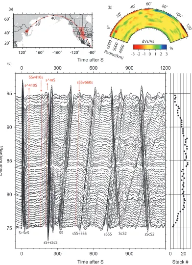
2.1 A USArray SH stacked record section from a deep earthquake. . . 11

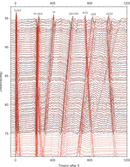
2.2 Comparison of data with SEM for SH. . . 12

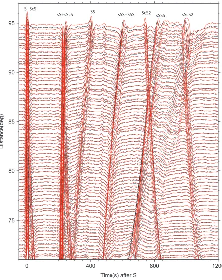
2.3 Comparison of mode with SEM for SH. . . 13

2.4 Comparison of data with finite difference synthetics. . . 15

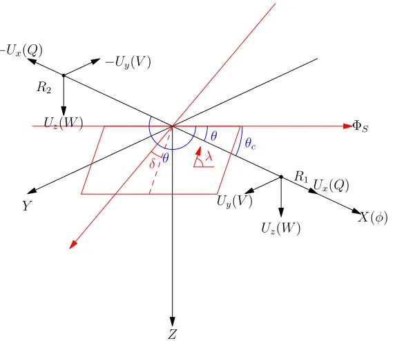
2.5 Coordinates systems. . . 19

2.6 Transparent source box for staggered-grid FD. . . 21

2.7 Illustration of transparent box effect. . . 22

2.8 Demonstration of complicated sources. . . 24

2.9 Demonstration of late-time drift. . . 25

2.10 Earth-flattening using different m. . . 27

2.11 Earth-flattening for tomography model. . . 28

2.12 Dispersion error for FD. . . 29

2.13 Comparison of FD with analytic solution for homogeneous model. . . 31

2.14 Comparison of FD with FK for layered model. . . 32

2.15 Comparison of FD with mode for PREM model. . . 33

2.16 Illustration of the correction steps. . . 34

2.17 Comparison of the amplitude for Pdiff and Sdiff. . . 35

2.18 Comparison between 2D-FD and 3D-SEM synthetics. . . 36

2.19 Comparison of data with FD using GyPSuM. . . 38

3.1 Diagram of ray paths. . . 49

3.2 Events and stations location. . . 51

3.3 Seismograms for 20091126 event. . . 53

3.4 Seismograms for 20090503 event. . . 55

3.5 Illustration of the multi-path detector. . . 56

3.6 PKiKP amplitude versus PcP amplitude. . . 57

3.7 Effects caused by upper mantle heterogeneities. . . 59

3.8 Selected displacement seismograms. . . 60

3.9 PKiKP/PcP ratio and ratio of ratio between two events. . . 61

3.10 Ratio of ratio shows large variations between nearby stations. . . 62

3.11 Simulation of effects of the CMB structure. . . 63

(11)

3.13 Model with 14km height and 0.5 degree heterogeneity. . . 66

3.14 Testing the stacking procedure on simulated waveforms. . . 67

3.15 PKiKP stacked records. . . 68

3.16 Amplitudes of the stacked records along two azimuth bins. . . 70

3.17 Migrated PKiKP amplitude pattern to the ICB. . . 71

3.18 Scenario for structures at CMB and ICB at PKiKP critical angle range. 73 3.19 PKiKP for PREM and model with bump at ICB. . . 74

3.20 MPD patterns. . . 77

3.21 Seismograms at two stations. . . 78

3.22 Sensitivity test for source side and receiver side scatter. . . 80

3.23 Synthetics for model with random medium. . . 81

3.24 Synthetics for core phases for source and receiver side heterogeneity. 82 4.1 Forward simulation of the sinking cylinder model. . . 101

4.2 Illustration of inversion process for the cylinder problem. . . 102

4.3 ReconstructedT0for various function evaluations. . . 103

4.4 Illustration of how M−1andK−1remove the mesh effects. . . 103

4.5 RecoveredT0forK−1preconditioned LBFGS. . . 103

4.6 Error reduction for LBFGS without and with preconditioner. . . 104

4.7 Error reduction and convergence ofCandninversion. . . 105

4.8 Error reduction andC,nrecover history forT0,C,ninversion. . . 106

4.9 Recovered results for two joint inversion cases. . . 106

4.10 Cost function and inversion pathes. . . 107

4.11 Subduction forward modeling. . . 109

4.12 Error andC1andn1recovery pathes for subduction inversion. . . 110

(12)

LIST OF TABLES

Number Page

2.1 Layered crust model. . . 30

3.1 Events that contain visible PKiKP phases after filtering to 1 to 3Hz . 50

4.1 Gradient test for cylindrical descent problem. . . 99

(13)

C h a p t e r 1

INTRODUCTION

Many important issues including the origin of natural resources, earthquake hazards,

and long-term climate change, have their roots in the current structure and

evolu-tion of the earth system. Having only access to the top several kilometers of the

earth, we have determined many details concerning the earth’s distinct past and its

deep interior through detective-like work. Geophysicists contribute to this endeavor

through studies in seismology, geodesy, mineral physics and geodynamics.

Concur-rently, a flood of data is being generated from dense networks of seismometers and

GPS stations, earth-orbiting satellites, and laboratory experiments on the material

properties on earth materials. Interpretation of this flood of data requires ever more

complex models, more powerful computers, and more efficient algorithms. My

the-sis contributes to two aspect of computational geophysics: seismic wave modeling

and geodynamic inversion.

Seismic waves, owing to their relatively short wavelength and low attenuation, are

the main tools to probe earth’s interior structure. They allow for the construction

of images of the interior in terms of seismic velocity anomalies and discontinuities.

Seismic tomography, initially based on travel time information from seismic ray

theory, has greatly advanced our knowledge of the structure of the earth (see e.g.,

Su and Dziewonski 1991; Grand et al. 1997; Ritsema et al. 2011). However, because

of the limitation of ray coverage, and approximation in ray theory, tomographic

images may smooth the true anomalies and recover smaller amplitudes of anomalies.

Seismic waveform modeling, based on the wave equation, can potentially use more

information in a seismogram, such as the amplitude and multipathing of phases, and

lead to the discrimination of important attributes, such as a low-velocity zone atop

410km discontinuity (Song et al. 2004) and post-perovskite phase transition near core

mantle boundary (Helmberger et al. 2005). Traditionally, 1-D synthetic methods

based on analytical or semi-analytical solution of the wave equation, for example,

general ray theory (Helmberger and Harkrider 1977) and frequency wavenumber

summation (Zhu and Rivera 2002), are often used. As the 1-D seismic structure

of the earth has been progressively refined, lateral velocity variation becomes more

important, and 1-D synthetics are often no longer suitable. Currently, 3-D synthetics,

(14)

and the 3-D finite difference method (Graves 1996), are often used in long period

global synthetics and in local ground motion studies. But since the computing cost

scales with the fourth power of frequency in 3-D, high frequency synthetics using

3-D methods at a global scale remain a challenge. Thus 2-D synthetics are often

used. Moreover, the available data may not be sufficient to constrain a 3-D model.

For example, the anomalies in waveforms may appear only on small regions of a

network, and may be mainly influenced by velocity structure near the great circle

propagation plane from the source to these stations. In such a case, 3-D modeling at

a global scale for all stations may be not be a wise use of computational resources.

In the next Chapter, I propose an efficient method to generate global synthetic

seismograms, using 2-D code and a post-processing correction step. This work

fills the gap between fast 1-D analytic synthetics and time-consuming full 3-D

synthetics in global seismic waveform modeling. Because seismic waves have

different geometric spreadings between 2-D and 3-D simulations, a correction is

required to convert 2-D synthetic seismograms to 3-D synthetics. We proposed a

new formulation for the correction, which automatically estimates the horizontal

ray parameters of difference phases in the seismogram, and then corrects the phase

amplitude based on these horizontal ray parameters. All of the correction is done as

a post-processing step of the recorded synthetic seismograms. The new formulation

removes the late-time drift appearing in a previous but similar method (Vidale and

Helmberger 1987). In order to apply the new method to modeling real earthquakes

at global scales, we also discussed how to interface the method with earthquake

source descriptions. Many complex source descriptions, like down-going only

wave, S only wave, etc., are supported by an extended, transparent box approach to

the staggered finite difference grid. Finally, we discussed several issues conscernin

the earth-flattening, which converts spherical to Cartesian geometry. The code is

implemented using staggered finite difference grids on a graphic processing unit

(GPU) architecture, but the method should be applicable to other 2-D methods, like

2-D spectral elements.

In Chapter 3, as a case study of seismic waveform modeling, I present my research

on the Inner Core Boundary (ICB). The solidification process at this boundary

between liquid outer core and solid inner core strongly influences the geomagnetic

field, and is of key importance to the geodynamo. Laboratory experiments indicate

that a thin mushy layer forms at the boundary between a fluid and the growing

(15)

depending on the properties of the light element present. Such a layer is likely to be

highly variable given the dynamic circulation involved. Thus, seismologists have

been addressing properties of this interface with an array of interesting observations,

e.g., Poupinet et al. (1983), Cormier and Choy (1986), Wen and Niu (2002), and

Cao et al. (2007). The near distance PKiKP phase, which is the reflection of a P

wave off the ICB, provides a direct constraint on ICB properties. Due to its weak

amplitude, and coverage limitation of stations, PKiKP at near distances has rarely

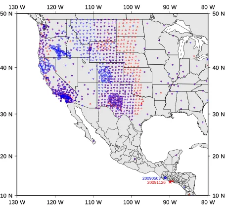
been observed in the past. We find several recent events beneath Central American

which produced excellent sets of PKiKP observations recorded by USArray at high

frequency. Other core phases, like PcP (reflection of P wave from core mantle

boundary,CMB), phases are also well recorded. We observe that the amplitude

of this phase displays considerable scattering across stations, with a factor of 6 or

more. Such amplitude variation can potentially be caused by many factors, like

site effects of stations, upper mantle inhomogeneity, or a bumpy structure along the

CMB or ICB. By considering the amplitude ratio between PKiKP and PcP phase,

and how this ratio changes for different nearby events, we are able to isolate an

amplitude pattern, which shows a rapid change of PKiKP amplitude within a small

range, and attribute this pattern to deep structure, i.e. CMB or ICB. Then through

modeling, we find that CMB influence on PKiKP phase is much smaller than that of

ICB influence, allowing us to attribute the amplitude pattern to ICB. Finally, using

seismic wave modeling, we find this pattern can be explained by small dome-like

anomalies above the ICB, where the material changes from that of the outer core to

that of inner core gradually.

Seismic images from tomography and waveform modeling give us a snapshot of

the present velocity structure of the mantle, for example, the large low velocity

provinces and ultra low velocity zones above CMB, the high-velocity anomalies

associated with a subducting slab. Such seismic anomalies are used as a constraint

on the temperature anomalies, specifically with low velocity province interpreted as

as hot, upwelling plumes , the high velocities in subduction zones as cool slabs. But

the scaling between seismic anomalies and temperature anomalies is is not perfectly

known. A geodynamic model of the mantle, combining seismic observation with

other available data, like plate motion history and topography, can potentially give

a better understanding of the origin and evolutionary history of these structures.

Computations of mantle convection are now being used to interpret a wide range of

(16)

delamination, and sea level change. Forward computational models in particular

have become more and more detailed and realistic. In these studies, the constitutive

relation (viscosity law) is found to play a first order role in such models. For example,

Billen and Hirth (2007) shows the rheological controls on slab dynamics. Despite

substantial effort attempting to determine the viscosity structure of the mantle, either

through forward or inverse geophysical models or through laboratory work, many

first order questions remain. For example, although global geophysical flow models

have suggested that the strength of lateral viscosity variations might be small (about

an order of magnitude) (e.g. Moucha et al. (2007) and Yang and Michael Gurnis

(2016)), global forward (Stadler et al. 2010) and local inverse models (Baumann

and Kaus 2015) suggest that the lateral variations in viscosity associated with plate

tectonics may be many orders of magnitude (> 103). In addition, as has been long evident in forward models (Mckenzie et al. 1974; Lenardic 2003) and plate tectonic

reconstructions (see review by Seton et al. (2012)), mantle convection is highly

time-dependent. This implies that it is essential that we find ways to constrain the

time-dependent viscosity structure. Some progress along these lines has been made

with global forward models (e.g. Bunge et al. (2009) and Bower et al. (2015))

and inverse models (e.g. Spasojevic et al. (2009) and Moucha and Forte (2011)).

Although there has been some attempt to use variable viscosity in such inverse

models meant to recover mantle structure in the past (Liu et al. 2008), they have not,

arguably, approached realistic variations in viscosity consistent with the dynamics.

To recover the viscosity and initial condition for mantle convection, casting the

problem as an inverse is most promising. Such inversions begin by defining a

cost function, a function of unknown viscosity parameters and initial temperature,

consisting of the misfit between model results and data. Then gradient based

opti-mizing method is used to minimize the cost function. Because of the large number

of unknowns, the adjoint method is an efficient way to obtain the gradient cost cost

function with respect to unknowns. Bunge et al. (2003) advanced an adjoint method

where the viscosity is assumed known, and only initial temperature is to be

recov-ered. Liu and Gurnis (2008) proposed an inversion of both viscosity parameters are

initial temperature for models with temperature and velocity dependent viscosity,

but its derivation of adjoint equation ignored such dependency, resulting in

subop-timal gradient. Worthen et al. (2014) and Ratnaswamy et al. (2015) instead studied

instantaneous Stokes flow problem, and recovered viscosity parameters assuming

(17)

In the last chapter of my thesis, based on these previous studies, we derive and test

adjoint inversion for a mantle convection problem where the unknowns include both

the initial temperature and scalar viscosity parameters of the mantle. A realistic

rheology, which includes both temperature- and strain rate-dependent terms, and

yielding, is used. We then derive the discrete gradient of the cost function in a

“Discretize then Optimize” fashion. This totally discrete fashion, as opposed to

many previous “Optimize then Discretize” approach, allows us to verify the correct

implementation of the adjoint equation, and makes full convergence of the inversion

possible. In the gradient based inversion, we adopt the limited memory

Broyden-Fletcher-Goldfarb-Shanno (LBFGS) approach. We find in this optimizing problem

with a field variable for temperatures unknown, a preconditioner to LBFGS is crucial

for faster convergence. Using traditional LBFGS, the optimization often fails before

the cost function can be reduced substantially. Using proposed preconditioned

LBFGS, all inversions explored achieve substantial reduction of cost function.

Finally, we use two synthetic cases, a sinking cylinder and a realistic subduction

model, to test our inversion method. The first model can be viewed as a simplified

version of the subduction dynamics problem, while the second model is motivated

by the evolution off of the west coast of North America, where Farallon-Pacific ridge

moved toward the subduction below the continent during the Cenozoic. We find that

in the inversion where only initial temperature is unknown, the initial temperature

can be recovered well; in the joint inversion of initial temperature and viscosity

parameters, the temperature, as well as effective viscosity, can also be recovered

reasonably well, but there are trade offs between viscosity parameters. Presumably,

the trade off in viscosity parameters is related to the ill-posedness of the problem.

In summary, both lines of my work in this thesis, seismic wave modeling and

ad-joint geodynamic inversion, are important tools that link geophysical theory with

observational data, which in turn leads to a better understanding of the earth system.

For the seismic wave modeling, many extensions of the method may have some

practical application. For example, the automatic estimation of ray parameter may

be used for real seismic recordings; the transparent box may be used for interfacing

a coarse grid global simulation with a dense grid local simulation, increasing

simu-lation efficiency. For the adjoint geodynamic inversion, more work is need to extent

the method to a global-scale problem. I think a module-like implementation, like

those modules in deep learning, will be useful for more seamless implementations,

(18)

and different observational data.

References

Baumann, T.S. and Boris J.P. Kaus (2015). “Geodynamic inversion to constrain the non-linear rheology of the lithosphere”. In: Geophysical Journal International 202.2, pp. 1289–1316. issn: 0956-540X. doi: 10.1093/gji/ggv201 (cit. on p. 4).

Billen, Magali I. and Greg Hirth (2007). “Rheologic controls on slab dynamics”. In: Geochemistry, Geophysics, Geosystems 8.8, n/a–n/a. issn: 15252027. doi: 10.1029/2007GC001597_{(cit. on p. 4).}

Bower, Dan J., Michael Gurnis, and Nicolas Flament (2015). “Assimilating litho-sphere and slab history in 4-D Earth models”. In: Physics of the Earth and Planetary Interiors 238, pp. 8–22. issn: 00319201. doi: 10 . 1016 / j . pepi . 2014.10.013_{(cit. on p. 4).}

Bunge, Hans Peter, C. R. Hagelberg, and B. J. Travis (2003). “Mantle circulation models with variational data assimilation: Inferring past mantle flow and structure from plate motion histories and seismic tomography”. In: Geophysical Journal International 152.2, pp. 280–301. issn: 0956540X. doi: 10 . 1046 / j . 1365 -246X.2003.01823.x_{(cit. on p. 4).}

Bunge, Hans-peter et al. (2009). “Time Scales and Heterogeneous Structure in Geodynamic Earth Models Time Scales and Heterogeneous Structure in Geo-dynamic Earth Models”. In: Science 91.1998, pp. 91–95. issn: 00368075. doi: 10.1126/science.280.5360.91_{(cit. on p. 4).}

Cao, Aimin, Yder Masson, and Barbara Romanowicz (2007). “Short wavelength topography on the inner-core boundary.” In:Proceedings of the National Academy of Sciences of the United States of America104.1, pp. 31–35. issn: 0027-8424. doi:10.1073/pnas.0609810104(cit. on p. 3).

Cormier, Vernon F. and George L. Choy (1986). “A search for lateral heterogeneity in the inner core from differential travel times near PKP-D and PKP-C”. In: Geophysical Research Letters13.13, pp. 1553–1556 (cit. on p. 3).

Grand, Stephen P., Rob D. van der Hilst, and Sri Widiyantoro (1997). “Global Seismic Tomography: A Snapshot of Convection in the Earth”. In: GSA Today 7.4, pp. 1–7. issn: 10525173. doi:10.1130/1052-5173-19.1.40(cit. on p. 1). Graves, Robert W (1996). “Simulating seismic wave propagation in 3D elastic media using staggered-grid finite differences”. In:Bulletin of the Seismological Society of America86.4, pp. 1091–1106 (cit. on p. 2).

(19)

Helmberger, D et al. (2005). “Deep mantle structure and the postperovskite phase transition”. In: Proceedings of the National Academy of Sciences of the United States of America102.48, pp. 17257–17263. doi:DOI10.1073/pnas.0502504102 (cit. on p. 1).

Komatitsch, Dimitri and Jeroen Tromp (1999). “Introduction to the spectral ele-ment method for three-dimensional seismic wave propagation”. In:Geophysical Journal International139, pp. 806–822 (cit. on p. 1).

Lenardic, a. (2003). “Longevity and stability of cratonic lithosphere: Insights from numerical simulations of coupled mantle convection and continental tectonics”. In: Journal of Geophysical Research 108.B6, pp. 1–15. issn: 0148-0227. doi: 10.1029/2002JB001859_{(cit. on p. 4).}

Liu, Lijun and Michael Gurnis (2008). “Simultaneous inversion of mantle properties and initial conditions using an adjoint of mantle convection”. In: Journal of Geophysical Research: Solid Earth 113.8, pp. 1–17. issn: 21699356. doi: 10. 1029/2007JB005594_{(cit. on p. 4).}

Liu, Lijun, Sonja Spasojevic, and Michael Gurnis (2008). “Reconstructing Farallon plate subduction beneath North America back to the Late Cretaceous.” In:Science (New York, N.Y.) _{322.5903, pp. 934–938. issn: 0036-8075. doi:} 10 . 1126 / science.1162921_{(cit. on p. 4).}

Mckenzie, D. P., J. M. Roberts, and N. O. Weiss (1974). “Convection in the earth’s mantle: towards a numerical simulation”. In: Journal of Fluid Mechanics 62, p. 465. issn: 0022-1120. doi:10.1017/S0022112074000784(cit. on p. 4). Moucha, R and A M Forte (2011). “Changes in African topography driven by

mantle convection”. In:Nature Geoscience4.10, pp. 707–712. issn: 1752-0894. doi:10.1038/ngeo1235(cit. on p. 4).

Moucha, R. et al. (2007). “Lateral variations in mantle rheology: Implications for convection related surface observables and inferred viscosity models”. In: Geophysical Journal International 169.1, pp. 113–135. issn: 0956540X. doi: 10.1111/j.1365-246X.2006.03225.x_{(cit. on p. 4).}

Poupinet, G., R. Pillet, and A. Souriau (1983). “Possible heterogeneity of the Earth’s core deduced from PKIKP travel times”. In:Nature305, pp. 204–206 (cit. on p. 3).

Ratnaswamy, V., G. Stadler, and M. Gurnis (2015). “Adjoint-based estimation of plate coupling in a non-linear mantle flow model: theory and examples”. In: Geophysical Journal International 202.2, pp. 768–786. issn: 0956-540X. doi: 10.1093/gji/ggv166_{(cit. on p. 4).}

(20)

Seton, M. et al. (2012). “Global continental and ocean basin reconstructions since 200Ma”. In:Earth-Science Reviews113.3-4, pp. 212–270. issn: 00128252. doi: 10.1016/j.earscirev.2012.03.002_{(cit. on p. 4).}

Shimizu, H., J.P. Poirier, and J.L. Le Mouël (2005). “On crystallization at the inner core boundary”. In:Physics of the Earth and Planetary Interiors151.1-2, pp. 37– 51. issn: 00319201. doi:10.1016/j.pepi.2005.01.001(cit. on p. 2).

Song, Teh-Ru Alex, Don V Helmberger, and Stephen P. Grand (2004). “Low-velocity zone atop the 410-km seismic discontinuity in the northwestern United States”. In: Nature427.6974, pp. 530–533. issn: 0028-0836. doi: 10.1038/nature02231 (cit. on p. 1).

Spasojevic, Sonja, Lijun Liu, and Michael Gurnis (2009). “Adjoint models of man-tle convection with seismic, plate motion, and stratigraphic constraints: North America since the Late Cretaceous”. In:Geochemistry, Geophysics, Geosystems 10.5. issn: 15252027. doi:10.1029/2008GC002345(cit. on p. 4).

Stadler, Georg et al. (2010). “The dynamics of plate tectonics and mantle flow: from local to global scales.” In:Science (New York, N.Y.) 329.5995, pp. 1033–1038. issn: 1095-9203. doi:10.1126/science.1191223(cit. on p. 4).

Su, Wei-jia and Adam M Dziewonski (1991). “Predominance of long-wavelength heterogeneity in the mantle”. In:Nature352.6331, pp. 121–126. issn: 0028-0836. doi:10.1038/352121a0(cit. on p. 1).

Vidale, John E and Donald V Helmberger (1987). “Path effects in strong motion seismology”. In:Seismic strong motion synthetics. Ed. by Bruce A. Bolt. London: Academic Press Inc (cit. on p. 2).

Wen, Lianxing and Fenglin Niu (2002). “Seismic velocity and attenuation structures in the top of the Earth’s inner core”. In:Journal of Geophysical Research107.B11, p. 2273. issn: 0148-0227. doi:10.1029/2001JB000170(cit. on p. 3).

Worthen, Jennifer et al. (2014). “Towards adjoint-based inversion for rheological pa-rameters in nonlinear viscous mantle flow”. In:Physics of the Earth and Planetary Interiors234, pp. 23–34. issn: 00319201. doi:10.1016/j.pepi.2014.06.006 (cit. on p. 4).

Yang, Ting and Michael Gurnis (2016). “Dynamic topography, gravity and the role of lateral viscosity variations from inversion of global mantle flow”. In:Geophysical Journal Internationalsubmitted, pp. 1–51 (cit. on p. 4).

(21)

C h a p t e r 2

GLOBAL SYNTHETIC SEISMOGRAMS USING A 2D

FINITE-DIFFERENCE METHOD

Li, Dunzhu and Helmberger, Don and Clayton, Robert W and Sun, Daoyuan (2014). “Global synthetic seismograms using a 2-D finite-difference method”. In: Geo-physical Journal International. doi:10.1093/gji/ggu050.

Two-dimensional (2D) finite-difference synthetics, which fill the gap between fast

1D analytic synthetics and time-consuming full 3D synthetics in our ability to

model seismograms, have been used in many studies. We address several issues

involving 2D finite-difference methods in generating global synthetic seismograms.

These include (1) interfacing point source excitation for earthquakes with 2D finite

difference methods; (2) out-of-plane spreading corrections; and (3) reducing the

spherical earth to the flattened models. The first issue is tackled using two methods,

a “transparent source box” approach and a moment tensor excitation approach,

where each has its own advantages. Moreover, our “source box” excitation does not

have the late time drift problem that occurred in previous studies. The out-of-plane

geometric spreading correction is accounted for by estimating the ray parameter

and applying a post-simulation filter to 2D synthetics. Finally, parameters of the

earth-flattening transformation are discussed and validated. The effectiveness of this

method is demonstrated by comparing our synthetics with frequency-wavenumber

summation, normal-mode, and 3D spectral-element synthetics.

2.1 Introduction

Our knowledge of the structure of the Earth has been greatly improved through the

de-velopment of global seismic tomography. These models are routinely used in global

centroid moment tensor (GCMT) solutions (globalCMT.org) and, more recently, in

synthetic seismogram predictions, such as the Spectral-Element Method (SEM)

(Ko-matitsch and Tromp 1999; Tromp et al. 2010). Here, as a motivation for our study,

we compare how well the tomographic model works for a deep (578km) earthquake

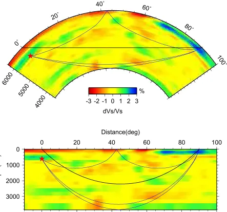
beneath the Russian-China border. The geometry is illustrated in Fig. 2.1a with a

typical tomographic model shown in Fig. 2.1b. A tangential record section from

(22)

dis-tance, shown in Fig. 2.1c. Synthetic predictions are shown in Fig. 2.2 as downloaded

from the Shake Movie website (http://global.shakemovie.princeton.edu). The

syn-thetics have been stacked in the same way as in the data and filtered to the accurate

band for synthetics (17 s and longer in this case). When stacked, we can easily detect

secondary arrivals that are reflected by the upper mantle discontinuities, as shown in

Fig. 2.1c. A comparison of 1D and 3D synthetics indicates that the waveform shapes

for most arrivals are similar as shown in Fig. 2.3. In short, 1D synthetics agree with

the 3D SEM tomographic model synthetics better than either model fits the data.

Thus the tomographic models can be refined by adding waveform modeling.

Synthetic seismograms are the main tools in modeling the complexities in the

seismic body waves. In 3D wave simulations, the space-time discretization leads to a

scaling of computational cost with the 4th power of seismic frequency, which makes

simulations especially challenging for high resolution. Moreover, the available

data may not be enough to constrain a 3D model. And sometimes the 2D model

assumption, which assumes the elastic parameters are invariant in the direction

perpendicular to the great circle propagation plane, is a good approximation for

many problems. Thus 2D media assumption is often used in waveform modeling,

which later can be checked against the SEM results as in Chen et al. (2007).

To compare synthetics with data, the point dislocation earthquake source and

out-of-plane spreading, which are 3D features, need to be considered. There are many

existing methods for the so called “2.5D simulation problem”, for example, 2D

finite difference in Cartesian coordinates (with a correction operator for out-of-plane

spreading) (Vidale and Helmberger 1987); 2D pseudospectral method in cylindrical

coordinates (with out-of-plane spreading correction) (Furumura et al. 1998; Wang

et al. 2001); axisymmetric finite difference (Jahnke et al. 2008); axisymmetric SEM

(Nissen-Meyer et al. 2007). The axisymmetric modeling takes into account the

out-of-plane spreading automatically, and by coupling P-SV system and SH system,

and using Fourier expansion in transverse direction, axisymmetric modeling can

also handle non-axisymmetric momentum tensor (Toyokuni and Takenaka 2006).

However, if we are interested in a non-axisymmetric model, such as a slab near the

source region, axisymmetric methods may not be suitable.

Here, we will focus on the 2D finite-difference (FD) simulation in Cartesian

coordi-nates, a method which has been studied extensively. To interface with an earthquake

source in 2D simulation, Vidale and Helmberger (1987) used a source box approach,

(23)

ar-75 80 85 90 95

Distance(deg)

0 300 600 900

Time after S

0 300 600 900 1200

Time after S

0 20

Stack #

S+ScS

sS+sScS

SS sSS+SSS _sSSS ScS2 _sScS2

s^410S SSv410s

s^mS _sSSv660s

120˚ 160˚ -160˚ -120˚ -80˚

20˚ 40˚ 60˚

120˚ 160˚ -160˚ -120˚ -80˚

20˚ 40˚ 60˚

0 20

40

60

80 100 0

0˚

20˚

40˚ 60˚ 80˚

100˚

120˚

4000 5000 6000

-3 -2 -1 0 1 2 3 dVs/Vs

% Radius(km)

(a) (b)

[image:23.612.111.503.68.608.2]

(c)

(24)

SS S+ScS

ScS2

sSS+SSS _sSSS

sS+sScS sScS2

75 80 85 90 95

Distance(deg)

0 0 2 1 0

0 8 0

0 4 0

Time(s) after S

0 0 2 1 0

0 8 0

0 4 0

[image:24.612.82.531.95.670.2]

Data(Black) and SEM(red)

(25)

SS S+ScS

ScS2

sSS+SSS _sSSS

sS+sScS sScS2

75 80 85 90 95

Distance(deg)

0 0 2 1 0

0 8 0

0 4 0

[image:25.612.81.529.104.669.2]

Time(s) after S Mode(Black) and SEM(red)

(26)

tificial late-time drifts. Coutant et al. (1995) used a momentum approach, which is

not compatible with double-couple solution normally assumed in modeling

earth-quakes. To address these source excitation issues, we first consider the relationship

between 2D and 3D simulations (the out-of-plane spreading). Next we show some

improvements and detailed analysis of two source excitation methods.

Our approach involves several approximations with the far field assumption, the

out-of-plane spreading correction, and the application of earth-flattening transformation

for non-layering spherical media. A comparison of our synthetics with data from

the above event is shown in Fig. 2.4. The travel time fits well, but because of the

lack of attenuation in our current code, the amplitude and waveform of upper mantle

phases (e.g., sSSS) become difficult to compare. However, in many applications,

convolving with at∗ operation or changing the sourcetime function can take into account the effective attenuation for a particular phase quite well.

Our goal is not to include all the complexity generally attributed to the earth, but to

develop a pragmatic tool in waveform modeling of global bodywave seismograms,

in particular some waveform segments. We show that our approach is sufficient for

many waveform modeling applications.

2.2 Methods

3D spreading

The relationship between point source and line source seismograms has been

dis-cussed in detail in recent textbooks, e.g., Chapman (2004). We will illustrate this

using an explosion source in a fluid whole space.

For a point source at the origin, the solution (denoted asV3D) follows the usual form

V3D(x,y,z,t) =

1

R3

δ(t−R3/α) (2.1)

whereαis P wave velocity, andR3=

p

x2+ y2₊_z2

is the source receiver distance,

andδis Dirac delta function.

Following Aki and Richards (1980, p. 226), a line source (alongydirection) solution

(27)

75 80 85 90 95

Distance(deg)

0 0 2 1 0

0 8 0

0 4 0

Time(s) after S

Data(Black) and FD Gypsum (red)

S+ScS

sS+sScS SS _sSS+SSS _ScS2 _sSSS sScS2

90 95

500 600 700

75 80

[image:27.612.81.535.125.603.2]

1000 1100

(28)

line

V2D(x,z,t) = Z ∞

−∞

V3D(x,y,z,t)dy

= 2pH(t−R/α) t2−R2/α2

= √ 2H(t−R/α) t+ R/α√t− R/α

≈ r

2α

R

H(t−R/α)

√

t−R/α

(2.2)

whereR=

√

x2+z2is the distance for the two dimensional problem,His the

Heav-iside step function, and the last approximation holds because the main contribution

toV2D is from the singularity at P arrival timet = R/α.

Thus, if we have a line source seismogram, we can obtain point source seismogram

at the same position by

V3D(x,0,z,t)=

1 π r p 2x d dt " 1 √

t ∗V2D (x,z,t)

#

(2.3)

wherep= x/Rαis the geometric ray parameter for the P arrival.

For a general 2D media, a similar result for each individual arrival can be obtained

by ray theory (Cerveny 2001)

V3D(x,0,z,t) =

1 π r 1 2F d dt " 1 √

t ∗V2D(x,z,t)

#

(2.4)

where the factor F =

R

r ayv dsis an integration of wave traveling velocityv along

the ray pathds. In a layered media, Eq. 2.4 reduces to Eq. 2.3 because

F = Z

r ay

vds= Z

r ay

v

sinθ sinθds=

Z

r ay

1

p dx = x

p (2.5)

whereθis the incident angle, andpis constant along the ray by Snell’s law.

But note that on one seismogram, p = p(t) is different for the various seismic

phases. Miksat et al. (2008) showed that using ray tracing to calculate theF factor

for each phase, line source seismogram can be corrected to obtain the point source

seismogram, phase by phase. However, ray tracing is complicated and processing

phase by phase is cumbersome. Instead, we assume Eq. 2.5 holds for typical global

simulations, with p the ray parameter observed at receiver side. This is a good

(29)

the strong heterogeneity is far from receivers and is small in size. Then Eq. 2.3

will hold. We will show that the correction pp(t) in Eq. 2.3 can be constructed

automatically without using ray tracing. This allows the correction of a whole

seismogram without using different windows for the various arrivals.

To construct√p, we first estimate the ray parameter p(t). Because

p= ikx

iω (2.6)

in the frequency (ω) and wavenumber(kx) domain, wherei=

√

−1_,ikxcorresponds

to a differential operator in the x direction, and 1/iω corresponds to an integral

operator in time, thus operationally

p(t)[. . .]→ − d dx

Z

[. . .]dt. (2.7)

Indeed, applying this toV2D in previous example

− d

dx Z "

H(t− R/α)

√

t−R/α

#

dt = x Rα

"

H(t− R/α)

√

t−R/α

#

= p

"

H(t−R/α)

√

t−R/α

#

. (2.8)

Therefore, if we generate the line source seismogramsV2D(x,z,t)along a horizontal profile, we can process adjacent traces using Eq. 2.7 to obtainp(t)V2D(x,z,t). Next, by taking the square root of the product of V2D(x,z,t) and p(t)V2D(x,z,t), and paying attention to the sign, we obtain

p

p(t)V2D(x,z,t) = sgn(V2D) p

|V2D×p(t)V2D|. (2.9)

By convolving with the remaining part in Eq. 2.3, we can then obtain the point

source seismogram at a particular receiver. This procedure works very well when

comparing results with other methods as demonstrated in this paper later.

Moment tensor source

In 2D simulation, we can simulate only line sources. We show that by correcting the

3D spreading, we can transfer line source seismograms to point source seismograms.

Now we will discuss how a point dislocation source ( an earthquake with 3D radiation

pattern ) is handled in 2D finite difference code. The first method uses the moment

tensor approach, which the 3D case is discussed in detail in Graves (1996).

Note that, in global modeling, receivers are distributed at different azimuths. The

(30)

radiation pattern. The former one can only be accounted for by conducting 2D

simulation at each azimuth of interest. Such kind of scaling of computing cost with

the number of azimuth is inevitable. However, in the azimuth bins of interest, if we

assume material properties do not change with azimuth, then the azimuth variation

is purely due to earthquake radiation pattern. This kind of azimuth variation is

equivalent to the case where receivers are at one azimuth but earthquake itself

changes its strike. Since earthquake moment tensor is combination of several

elementary tensors, then by combination of synthetics for these elementary moment

tensor, we can account for azimuth variation in the latter case at no extra simulations.

In Cartesian coordinates shown in Fig. 2.5, the earthquake source is at the origin, Z

points downwards and X points to receiver azimuth φ. All material properties are assumed invariant in Y direction. For a double couple source (strikeφs, rakeλ, dip δ), the elementary moment components are (Aki and Richards 1980)

Mx x =−(sinδcosλsin 2Φ+sin 2δsinλsin2Φ),

Mxy =sinδcosλcos 2Φ+1/2 sin 2δsinλsin 2Φ,

Mx z =−(cosδcosλcosΦ+cos 2δsinλsinΦ),

My y =sinδcosλsin 2Φ−sin 2δsinλcos2Φ,

Myz =−(cosδcosλsinΦ−cos 2δsinλcosΦ),

Mzz =sin 2δsinλ,

(2.10)

whereΦ= Φs −φis the effective strike in this coordinate system.

In 2D simulation, we can not simulate all six components, but fortunately we do not

need to. The far field radiation for P-SV and SH is after Chapman (2004, p. 123)

P(M;φ1, φ2)= (Mx xcos2φ1+My ysin2φ1+ Mxysin 2φ1)sin2φ2, + Mzzcos2φ2+(Mz xcosφ1+ Myzsinφ1)sin 2φ2,

SV(M;φ1, φ2)= 1/2

Mx xcos2φ1+My ysin2φ1−Mzz +Mxysin 2φ1

sin 2φ2, +

Mz xcosφ1+Myzsinφ1

cos 2φ2,

SH(M;φ1, φ2)= (1/2(My y− Mx x)sin 2φ1+Mxycos 2φ1)sinφ2, +(Myzcosφ1−Mz xsinφ1)cosφ2.

(2.11)

(31)

re-Y

ΦS

Z

R₁ R₂

δ

θc

θ

λ

Uy(V)

Ux(Q)

Uz(W)

−Uy(V)

−Ux(Q)

Uz(W)

[image:31.612.167.453.70.317.2]

X(φ)

Figure 2.5: Coordinates systems. The dislocation source is at the origin, with the following fault parameters: strike Φs, rakeλ, dip δ. The receiver R1 is at azimuth φ, R2 is at azimuth φ+ π. In cylindrical coordinate (θ,r,z), θ is the clockwise angle from the strike to the receiver. The direction for SH displacement (V) and P-SV displacement(Q and W) is also shown. In Cartesian coordinate, X points to the receiver direction, Z points downward. The displacement for P-SV is (Ux,Uz), for SH isUy. Define θc = φ− Φs, the clockwise angle from strike (Φs) to positive X direction (φ). In the FD source injection, we need to know the displacement in a box surrounding the point dislocation. Note that for the

x ≥ 0 _region, r = x, θ = θc,Ux = Q,Uy = V,Uz = W; and for the x < 0 region,

r =−x, θ= θc+π,Ux =−Q,Uy =−V,Uz = −W.

spectively. Thus in the XZ plane we choose,φ1 =0, then

P(M;φ2) = Mx xsin2φ2+Mzzcos2φ2+ Mz xsin 2φ2,

SV(M;φ2) =1/2 Mx x −Mzzsin 2φ2+ Mz xcos 2φ2,

SH(M;φ2) = Mxysinφ2+ Myzcosφ2.

(2.12)

So only Mx x,Mzz,Mx z contribute to the far field PSV system in the XZ plane, and only Mxy,Myz contribute to the far field SH system in the XZ plane. And for these components, we can interface them in 2D FD code.

(32)

the 2D FD code via the velocity-stress formulation of elastodynamics equation

ρ∂u˙i

∂t =Ti j,j,

∂Ti j

∂t =ci j klu˙k,l−m˙i j,

(2.13)

where u˙i is the velocity, Ti j the stress, subscript ,j differentation, ci j kl the elastic

parameter, and mi j seismic moment density. For a point dislocation source mi j = Mi jf(t)δ(x − xs), where f(t) is the seismic source time function,x is 2D spatial

coordinate, and xs is the source location . In the finite difference simulation, δ(x − xs) is replaced by 1/(∆h)2, an average over the grid cell, where ∆h is the

finite difference grid size. Then at every time step, the source injection is done by

updating the stress components at the source grid points

Ti j ←Ti j−∆t Mi jf˙(t)/(∆h)2 (2.14)

Transparent source box

The momentum approach is simple and compact in space. However, a classic

approach discussed in this section has the advantage of modeling some complex

sources.

Here, we follow the transparent box approach used by Alterman and Karal (1968)

and Vidale et al. (1985) to add the source into the FD. This procedure becomes more

complicated in staggered grid FD. The basic idea is to divide the elastic wavefieldA

into two parts, one of which is the known analytical source part S, and the other is

the unknown partRthat accounts for interactions with the structure, soA= S+R.

Conceptually we will conduct two FD simulations. One is within the source region

and only updates R, the other is outside the source box and updates A. The two

simulations exchange information through the boundary.

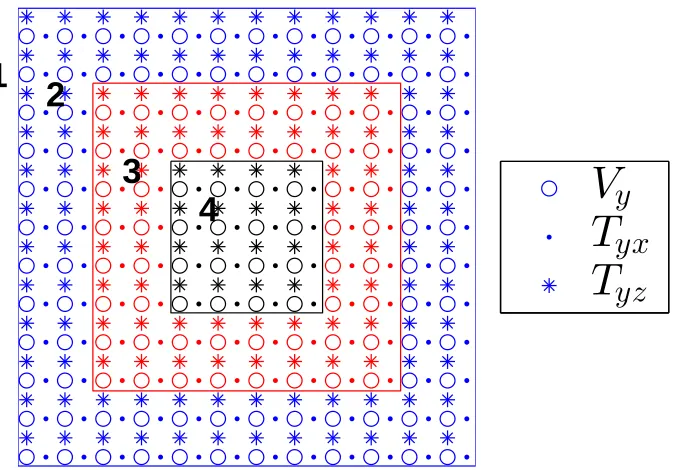
In Fig. 2.6, the FD grids are divided into four parts, where part (1)(2) is the region

where we update A, and part (3)(4) is the region where we updateR.

In the first FD simulation that updatesA, we need to knowAat part (3) as a boundary

condition. In part (3) we only know Rfrom the second FD simulation at previous

time step, but we can use A= R+Sto obtain Aat region (3), provided that we can

calculateS analytically. Similarly, in the second FD simulation that updates R, we

need R in part (2) as a boundary condition. We only know Ain part (2) from the

(33)

1

2

3

4

V

y

[image:33.612.141.479.69.304.2]

T

yx

T

yz

Figure 2.6: The source box for a staggered-grid finite difference for the SH case. Part (1)(2) is the region for updating A. Part (3)(4) is the region for updatingR. We need to compute source wavefield S analytically at part (2)(3). Note that as a boundary condition for simulation of R in (3), the width of part (2) should be larger enough to accommodate the width of FD stencil centered on part (3). Similarly, width of part (3) should be larger enough to accommodate the width of FD stencil centered on part (2). Here, the finite difference stencil width is 4 grid points (two points on each side), so we choose width of region (2) and (3) to be 2 grid points. There is no limit on how large part (4) can be, as long as it’s large enough to accommodate the width of FD stencil in part (3).

In detail, for either PSV or SH system, one FD step for updating stressTand velocity

V requires:

1. V_An=V_Rn+V_Snin region (3)

2. (TAn−1/2,V n A)→T

n+1/2

A in regions (1) and (2)

3. V_Rn=V_An−V_Snin region (2)

4. (T_Rn−1/2,V_Rn)→T_Rn+1/2in regions (3) and (4)

5. TAn+1/2=T n+1/2

R +T

n+1/2

S in region (3)

6. (V_An,T_An+1/2)→V_An+1in regions (1) and (2)

(34)

−20 −10 0 10 20 30 40 50 60 70 80 −20

−10

0

10

20

30

40

50

60

70

[image:34.612.165.448.70.353.2]

80

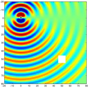
Figure 2.7: The wavefields radiated from a monotone source outside of the box (white region). Although there is no explicit updating of the total wavefield inside the box, the wavefield passes the box smoothly as if it does not exist.

8. (VRn,T n+1/2

R )→V

n+1

R in regions (3) and (4)

This approach allows the scattered wavefields to pass the source box as if the box

does not exist, which is termed “transparent source box” (Aki and Richards 1980),

see Fig. 2.7.

Vidale et al. (1985) and Helmberger and Vidale (1988) proposed an approach widely

used to interface the 2D FD method with Cagniard-de Hoop source description that

accounts for the 3D earthquake radiation pattern. But their approach produces a

late-time drift, which obscures late arrivals like surface waves. To understand the

cause of drift, we take a point dislocation source (pure strike-slip) in homogeneous

media as an example. In their approach, using cylindrical coordinates ( Fig. 2.5 ),

the vertical displacement at position (θ,r,z) in homogeneous media will be ( see Appendix for details )

(35)

whereα, βdenote the P and S contribution respectively. In detail

Wα = _{4π ρ}M0 _π2A(θ, λ, δ) d

dt " 1 √ 2r 1 √ t ∗I m

"

(−p2)

√ p

ηα(−εηα)

dp dt

# #

,

Wβ = _{4π ρ}M0 _π2A(θ, λ, δ) d

dt " 1 √ 2r 1 √ t

∗I m

"

(−εpηβ)

√ p

ηβ(p)

dp dt

# #

,

(2.16)

where M0 is the seismic moment, ρ is the density, r is the horizontal distance between source and receiver,εis the sign of Z coordinate of the receiver, A(θ, λ, δ) is a function depending on earthquake focal mechanism (strike assumed at 0, rake λ, dipδ) and azimuth of the receiverθ, and

p= r

R2t+i t 2₋ R2

v2

!1/2 |z|

R2

ηv = |z|

R2t−i t 2₋ R2

v2

!1/2 r

R2, v= α, β

(2.17)

withi=

√ −1_.

Because of the singularity att = R/vfor the term 1

η

dp dt =

i

(t2−R2/v2₎1/2 (2.18)

the most contribution comes from the time when phase first arrives. Eq. 2.17 then

becomesp≈r/Rv = p0, and thus the term in Eq. 2.16 can be simplified

I m

"

√

p(· · ·)1

η

dp dt

#

≈ I m

"

√

p0(· · ·)

1 η

dp dt

#

= √p0I m

"

(· · ·)1

η

dp dt

#

=p

p0(t)W2D.

(2.19)

Then it can be verified that theW2Dpart is indeed a line source solution and satisfies

the 2D wave equation. Thus it can be interfaced with 2D FD to propagate to further

distance from the source. Note p0(the geometric ray parameter) is the same as pin

Eq. 2.3.

The aboveW2D = W2D,α +W2D, β consists of the P and S part, respectively. It can

be shown thatW2D,α andW2D, β each individually goes into infinity ast → ∞, but

their summationW2D does not. For example, wavefield snapshots ofW2D,W2D,α,

andW2D, βgenerated using the “transparent box approach” are shown in Fig. 2.8abc

respectively. Note that the drift terms appear around source box in Fig. 2.8bc, but

they are of opposite sign and are cancelled as shown in Fig. 2.8a.

In Vidale and Helmberger (1987), however, the authors approximated pp0(t)/r

using

√

(36)

(a) (b)

(c) (d)

Figure 2.8: Demonstration of box sources for: (a) a dislocation source; (b) its P wave component; (c) its S wave component; (d) its downgoing component. The white box is the source region. Note that the P and S components seperately are unstable, but their sum (a) is stable.

with a sourceW2∗D = √

1/αW2D,α+ p

1/ βW2D, β. In this way, the drifting term will

not be cancelled, and W₂∗_D → ∞ as t → ∞. The seismograms generated using the original formulation (old source) and the new one are compared in Fig. 2.9.

Although the drift is of low frequency and can be mitigated using a high-pass filter,

it becomes large in amplitude at late-time, and contaminates the late arrivals, making

it difficult to use in global modeling. The new source approach does not have this

problem.

The source box approach has the advantage that it can be used to represent some

complex sources. For example, in Fig. 2.8bc, we show that we can interface with

only the P part or the S part of the wavefield. Note that the seperate P and S part

each individually has the correct radiation pattern, which is hard to obtain using the

moment tensor approach. We can also simulate only the downgoing wavefield by

nullifying the wavefield in the upper half of the source box, as shown in Fig. 2.8d.

Although the separation of downgoing part is not perfect, such flexibility proves

(37)

0 5 10 15 20 25 30 35 40 Time

Old source

New source

New source high pass

Old source high pass

P

S

P

S

Figure 2.9: The old source box has the low-frequency late-time drift and can be mitigated using a high pass filter. The new source box does not have the drift. Note that the S phase amplitude of the old source is bigger because of an extra pα/ β factor compared with that of the new source.

1997), and the identification of depth phases.

While the above 2D approaches are equivalent to an asymptotic double-couple

solution (the so-called far-field solution), they may break down at very long periods,

which proves useful as demonstrated below.

Earth Flattening Transform

Since global models are sensitive to the earth’s curvature, in Cartesian coordinate

simulation, the treatment of earth flattening becomes essential. A particularly simple

transformation was proposed by Müller (1971),

z = alog a

r,

αf =αs a r,

βf = βs a r,

(2.20)

wherez,αf, βf are the depth and velocities in the flat model,r, αs, βsare the radius and velocities in the spherical model, and a is the radius of the earth. This earth

(38)

earth. To obtain the correct amplitude, we also need a transform for density, which

usually takes the following form

ρf(z) = ρs _r

a m+2

, (2.21)

wheremis to be determined.

For an SH system in layered media, Biswas and Knopoff (1970) show that an exact

earth flattening transformation is achieved by setting m = 3. However, an exact

earth flattening transformation does not exist for the P-SV system, andm from−3

to 3 have been considered (Chapman 1973). A m = −3 appears to be optimal

in a layered fluid, which has the same transformation of density as that used for

velocities (Helmberger 1973). Another commonly used value is m = −2, which

keeps ρf(z)= ρs(r)(Müller 1971).

Given the same seismic moment in Cartesian code, the absolute amplitude of the

body wave increases asmincreases (which means a decrease inρf). Our numerical tests show that, at distance of 90°, a unit increase ofmvalue results in an increase

of 5% in the P wave amplitude. But as shown in Fig. 2.10a, the relative amplitude

and waveform complexity of body wave changes little as we change m, and the

largest differences between the results are in the fundamental Rayleigh wave phase.

The fundamental Rayleigh wave has a very long-period and is sensitive to earth’s

curvature and density (Dahlen and Tromp 1998). A search for the appropriate m

value shows thatm= 0fits the Rayleigh wave better than other integerm, although

at these periods self-gravitation, and the Earth’s rotation become important issues,

and because these are already embedded in the SEM, it is the preferred method at

these periods.

As discussed in Gilbert and Helmberger (1972), transferring the synthetics from

flattened earth model to spherical earth model needs another amplitude correction

U(s) ≈

p

∆/sin∆U(f), (2.22)

where∆is the epicentral distance in degrees.

The above earth flattening transform is for a 1D spherical earth. For a lateral varying

tomographic model, we apply earth flattening transform to each vertical profile, as

in many previous studies. A demonstration of the transformation with several ray

(39)

1000 2000 3000 Z Earth flatten vs Mode

m=-3

m=-2

m=-1

m=0

Mode

m= 1

m= 2

m= 3

40 50 60 70 80 90 100

Distance(deg)

0 1000 2000 3000

Z m=0 vs Mode

(a)

(b)

Figure 2.10: (a) Comparison of vertical displacement seismograms at 90◦ for the PREM using different m with mode summation synthetics. It appears that m = 0 best fits the fundamental Rayleigh around 2700s in these cases. (b) m=0 synthetics (red) fits mode summation Rayleigh wave(black) at other distances as well.

FD implementation

Finite difference methods in seismology have been discussed by many authors.

In our implementation, we use the staggered grid velocity-stress scheme (Virieux

1984; Levander 1988), which can account for solid-fluid interface automatically.

For the SH system, the free surface is implemented using stress imaging method;

for PSV system, we use the method in Mittet (2002). For absorbing boundary

condition, we use the parameter in Zhang and Shen (2010). The code is written

using CUDA (Micikevicius 2009) and parallelized using pthread on three GPUs

within one computing node, which for our 2D case has a speedup around 100

compared with a single CPU.

To reduce spatial dispersion caused by discretization, we use 8th order central

(40)

0

1000

2000

3000

Flatten Depth(km)

0 20 40 60 80 100

Distance(deg)

0˚

20˚

40˚ _60˚

80˚

100˚

4000 5000 6000

-3 -2 -1 0 1 2 3 dVs/Vs

[image:40.612.89.532.154.567.2]

%

(41)

0 5 h=1/6L, dt=0.06h/v

ord 2

ord 4

ord 6

ord 8

0 5

h=1/12L, dt=0.06h/v

0 5

h=1/6L, ord 8

dt=0.24h/v

dt=0.12h/v

dt=0.06h/v

(A) (B)

Figure 2.12: Illustration of dispersion error assuming SH simulation in a homoge-neous space. The S velocityvis 6 km/s, and the source-time function is of Gaussian shape with central frequency 1Hz, which gives a wavelength Lof 6km. The source receiver distance is 6000km, which is1000L. (A) Demonstration of spatial disper-sion. Red traces are simulation results, and black is the analytical calculation. For two cases of grid space of h = 1/6L and h = 1/12L, dispersion error reduces as we increase spatial discretization order. The time discretization is very fine and its dispersion error can be neglected. (B) Demonstration of temporal dispersion. For

h=1/6Land 8th order spatial discretization, time dispersion error decreases as we reduce the time step.

staggered grid method, whose dispersion error can be mitigated by reducing the time

step, which does not increase simulation memory requirements. Detailed analysis

of this scheme is discussed in (Virieux 1984; Levander 1988). Here we show an

example to illustrate the dispersion error. In a homogeneous space with S velocity of

6km/s, we conduct a SH simulation with a source-time function of Gaussian shape

(central frequency about 1Hz and wavelength 6km). The source receiver distance

is 6000km, which corresponding propagating 1000 cycles. In Fig. 2.12a, we show

how the spatial dispersion is reduced by increasing spatial discretization order or

halving the grid space. In Fig. 2.12b, we show how the temporal dispersion is

mitigated by reducing the time step. Note the phase delay of spatial dispersion and

(42)

thickness(km) vp(km/s) vs(km/s) density (g/cc)

3.95 4.4 2.51 2.0

10.0 6.0 3.46 2.6

16.0 6.7 3.87 2.9

∞ _7.7 _4.5 _3.3

Table 2.1: Layered crust model.

2.3 Validation

Regional modeling

We begin with the simplest problem, producing synthetics for a strike slip fault in

a homogeneous space, to test the radiation patterns and 2D to 3D correction. A

snapshot of the radial velocity wavefield in the XZ plane is shown in Fig. 2.13a, with

three receivers distributed to sample the radiation pattern. The raw finite difference

synthetics (velocity seismogram for the line source) are shown in Fig. 2.13b, along

with the line source analytical results. After 3D spreading correction, we obtain the

point source seismograms in Fig. 2.13c, which are in good agreement with the point

source analytical

Some Advances in Computational Geophysics: Seismic Wave and Inverse Geodynamic Modeling