Cluster Labeling based on Concepts in a Machine-Readable Dictionary
Fumiyo Fukumoto
Interdisciplinary Graduate School of Medicine and Engineering
Univ. of Yamanashi
Yoshimi Suzuki
Interdisciplinary Graduate School of Medicine and Engineering
Univ. of Yamanashi
Abstract
This paper addresses the issue of cluster labeling and presents a method for assign-ing labels by usassign-ing concepts in a machine-readable dictionary. We assume that salient terms in the cluster content have the same hypernym because hypernymic se-mantic relation represents a generalization that goes from specific to generic. Our ex-perimental results reveal that hypernymic semantic relations can be exploited to in-crease labeling accuracy, as the results of 0.441 F-score improves over the two base-lines.
1 Introduction
With the exponential growth of information on the Internet, finding and organizing relevant materials on the Internet is becoming increasingly difficult. Internet directories such as Yahoo! and Google, which classify Web pages into pre-defined hier-archical categories, provide one solution to the problem. Categories in the hierarchical struc-tures are carefully defined by human experts and documents are well-organized. However, manual category-tagging is extremely costly. Moreover, categories on some Internet is often insufficient in finding relevant documents for users. Because these categories tend to have some bias in both defining and classifying documents. Cluster label-ing is one of the techniques to attack the problem. Most of the work on cluster labeling identi-fies salient terms in the cluster content that char-acterize the cluster in contrast to other clusters. Salient terms are extracted by using statistical fea-ture selection, e.g., maximum sum of the indi-vidual term frequencies of documents assigned to a cluster (Cutting et al., 1992), an adapted ver-sions of Information Gain (Geraci et al., 2007), χ2 method (Popescul and Ungar, 2000), and the
Jensen-Shannon Divergence (Camel et al., 2009). Other works based on salient terms are frequent phrases by (Osinski and Weiss, 2005), and inte-gration of hierarchical information by (Muhr et al., 2010). However, the suggested terms, even when related to each other, tend to represent different as-pects of the topic underlying the cluster, and it is often the case that a good label does not occur di-rectly in the document. Carmel et. al addressed the issue and presented a method to use Wikipedia as an external knowledge. They showed the effec-tiveness of the method. However, Wikipedia is the free online encyclopedia, and everyone can access and edit the information. Therefore, it is often in-cluded noise information such as categories which do not characterize the cluster in the pages. Chin et. al presented a method to use WordNet (Chin et al., 2006). They used machine learning through extending the given term set with synonyms, hy-pernyms, hyponyms and so on. However, their method needs training data to determine the actual weights. Through supervised training in the label-ing process the actual influence of synonyms, hy-pernyms, hyponyms information remains unclear.
This paper focuses on cluster labeling, and presents a method for assigning labels automati-cally by using concepts in a machine-readable dic-tionary. Similar to Chin et. al work, we focused on semantic relation in a dictionary, namely hyper-nymic semantic relation that represents a general-ization, i.e., goes from specific to generic (Fell-baum, 1998), and used it in the cluster labeling process. We assume that salient terms in the clus-ter content have the same hypernym in a hierarchi-cal structure of a dictionary. The hypernym repre-sents generic concepts of a set of documents, thus can be a label of a cluster.
2 Cluster Labeling
The procedure for cluster labeling consists of four steps: documents clustering, term weighting,
pernym extraction, and ranking labels.
2.1 Documents clustering
The first step is to classify documents into a set with semantically similar documents. In the docu-ment clustering, we do not know how many clus-ters there are in a given input documents. More-over, the algorithm should allow each data point to belong to more than one cluster because of multi-label classification. We used a graph-based unsu-pervised clustering technique developed by (Re-ichardt and Bomholdt, 2006); we call this the RB algorithm. This algorithm detects the node con-figuration that minimizes the energy of the ma-terial. The energy function, called the Hamilto-nian, for assignment of nodes into communities clusters together those that are linked, and keeps separate those that are not by rewarding internal edges between different clusters. Here, “commu-nity” or “cluster” have in common that they are groups of densely interconnected nodes that are only sparsely connected with the rest of the net-work. Only local information is used to update the nodes which makes parallelization of the al-gorithm straightforward and allows the applica-tion to very large networks. Moreover, compar-ing global and local minima of the energy function allows the detection of overlapping nodes. Re-ichardt et al. evaluated their method by applying several data including a large protein folding net-work, and reported that the algorithm successfully detected overlapping nodes (Reichardt and Born-holdt, 2004). We thus used the algorithm to cluster documents. Letdi (1≤i≤n) be a document in
the input, and σi be a label assigned to the
clus-ter in which di is placed. The HamiltonianH is
defined as:
H({σi}) = −
i<j
(Aij(θ)−γpij)δσiσj.(1)
δ denotes the Kronecker delta. The function Aij(θ)refers to the adjacency matrix of the graph,
which is defined as:
Aij(θ) =
1 if sim(di,dj)>0
0 otherwise. (2) sim(di,dj) in Eq (2) refers to cosine similarity
be-tweendianddj. The matrixpij in Eq. (1) denotes
the probability that a link exists betweendianddj,
and is defined as:
pij =
i<j
Aij(θ)
N(N −1)/2, (3)
where N refers to the number of documents and
N(N−1)
2 is the total number of document pairs. As
the parameter γ in Eq. (1) increases, each docu-ment is distributed into larger number of clusters. Eq. (1) thus shows comparison of the actual val-ues of internal or external edges with its respective expectation value under the assumption of equally probable links and given data sizes. The minima of the Hamiltonian H are obtained by simulated annealing (Kirkpatrick et al., 1983). We applied simulated annealing forT runs1.
2.2 Term weighting
For the results of clustering, we extracted salient terms from each clusters obtained by the RB al-gorithm. We tested four metrics which are com-monly used as feature selection, i.e., TF∗IDF, mu-tual information, χ2 statistics, and information
gain. The terms we used are noun words in the documents. Each term is scored according to its contribution to the metrics between the cluster and other clusters. The topkscored terms are then se-lected as a candidate of the cluster salient terms.
2.3 Hypernym extraction
The third step is to extract hypernym for each term selected by term weighting method. We used Japanese word and concept dictionaries of EDR 2. The word dictionary consists of 270,000 words.
Each word has concept identifier as well as lexical and grammatical information. The concept iden-tifier is to identify words and their concepts. The concept dictionary consists of 410,000 concepts. Each concept is linked to other concepts, and the link is a relation between concepts, namely super-sub relation. We used this super-super-sub relation as hypernymic semantic relation. LetW ={w1,w2,
· · ·,wn}be a set of words in a cluster selected by
feature selection. For each pair of words, wi and
wj, we identified its hypernymckby using Eq. (4).
ck = hy(wi)∩hy(wj) (4)
where hy(wi) and hy(wj)
sat-isfy min(dis(hy(wi), wi)) and
min(dis(hy(wj), wj)), respectively. In Eq.
(4), hy(x) refers to the hypernym of a word x. min(dis(hy(wi), wi)) shows the minimum
distance between hy(wi) and wi. We extracted
hypernym by using Eq. (4), and regarded these as label candidates.
1
We setT to 1,000 in the experiments
Second level Third level Fourth level sports gymnastics winter ski
music opera song
medicine pharmacy pharmaceuticals education school teacher architecture house flat nature environment lebensraum plants botany dicots religion religion in India Buddhism military national defense army
earth geology geomorphology organism anthropology anthropologist economy labour labour market management post mail service agriculture animal care poultry
animals zoology animal physiology international law UN UNSC
finance stock bond
Table 1: Categories
2.4 Ranking Labels
The final step for cluster labeling is to rank label candidates according to their scores. The score of candidatecis obtained by using Eq. (5).
Score(c) = −logf req p(c)
N (5)
where N = f req p(w 1
i)+f req p(wj). wi and wj are words selected by feature selection. f req p(x)is the number of senses that the wordxhas.
3 Experiments
3.1 Data
We used two types of test data: one is a collec-tion that correct labels occur directly in the docu-ments. Another is that a label does not appear in the documents. The data we used is RWCP cor-pus labeled with UDC codes selected from 1994 Mainichi newspaper (RWC, 1998). It consists of 27,755 documents organized into fine-grained cat-egories, 9,951 categories with a seven-level hier-archy. We used categories/labels assigned to the second, third and fourth level of a hierarchy, each of which has more than five documents3. Each level consists of 17 categories shown in Table 1. For each category, we randomly selected five doc-uments, and created each type of test data. We ex-tracted the top 20 scored words by term weighting as a candidate of the cluster salient terms.
3We did not use categories assigned to the top level, as it
was defined by only one label.
RB EM
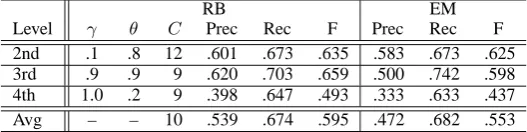
[image:3.595.307.571.64.130.2]Level γ θ C Prec Rec F Prec Rec F 2nd .1 .8 12 .601 .673 .635 .583 .673 .625 3rd .9 .9 9 .620 .703 .659 .500 .742 .598 4th 1.0 .2 9 .398 .647 .493 .333 .633 .437 Avg – – 10 .539 .674 .595 .472 .682 .553
Table 2: Clustering Results
3.2 Clustering accuracy
For each category, we randomly selected five doc-uments and created a training data to estimate two parameters, γ and θ. We represented each doc-ument as a vector of noun word frequencies, and applied RB algorithm. For evaluation of document clustering, we used F-score, especially to capture how many documents does the algorithm actually detect more than just one category. Precision was defined by the percentage of documents appear-ing in the correct clusters compared to the num-ber of documents appearing in any cluster, and re-call was defined by the percentage of documents within the correct clusters compared to the total number of documents to be clustered. For com-parison of clustering algorithm, we used the EM algorithm that is widely used as a soft clustering technique(Nock et al., 2009). We set the initial probabilities by using the result ofk-means clus-tering, wherekis set to the number of correct clus-ters,1 7. We used up to 30 iterations to learn the model probabilities. The results are shown in Ta-ble 2.
Table 2 shows average performance between two types of test data. γ andθin Table 2 denote the values that maximized the F-score obtained by using the training data. “C” refers to the number of clusters obtained by RB. The overall results ob-tained by the RB algorithm were better to those obtained by the EM algorithm regardless of the level of a hierarchy.
3.3 Labeling accuracy
We tested two types of document collection. For evaluation of cluster labeling, we used 11-point average precision. For comparison of the method, we used two baselines: (i) a feature selection by TF∗IDF, and (ii) the use of Wikipedia for labeling. The method using Wikipedia is based on (Camel et al., 2009) 4. The difference is that we used RB for clustering, and TF∗IDF to extract salient
4We used Wikipedia downloaded from
Labels are included Labels are not included
Level EDR TF
∗IDF Wiki EDR Wiki
TF∗IDF MI χ2 IG TF∗IDF MI χ2 IG
[image:4.595.85.515.62.141.2]Second 0.460 0.318 0.281 0.288 0.150 0.236 0.500 0.304 0.288 0.272 0.153 Third 0.533 0.276 0.281 0.396 0.220 0.187 0.523 0.340 0.334 0.343 0.140 Fourth 0.310 0.254 0.214 0.256 0.183 0.194 0.299 0.262 0.193 0.220 0.142 Average 0.434 0.283 0.259 0.284 0.184 0.206 0.441 0.302 0.272 0.278 0.145
Table 3: The results of cluster labeling
Second level Third level Fourth level vertebrate, life-form contest, sport ski, athlete
music, opera music, opera song, music
sick, hypofunction sick, food sick, antibiotic book, building rule, human guide, rule cook, building building, activity building, activity
nature, natural phenomenon think, information study, phenomenon
plants,botany botany, tree animals and plants, animal
religion, human belief, statue life, plants
reader, staff military, military affairs military, army
earth, planet geology, message geology, loss
organism, life life anthropology human, animal
economy social economy labour, worker labour market, market
management, organization money, market information, service
agriculture, vegetables food, cook care vegetables
animals, mammals zoo, plant care, food
international law, law UN, USA UNSC, society
[image:4.595.132.466.177.369.2]bank, money stock, share bond, market
Table 4: Lists of top 2 terms (The top 20 term weighting scored terms)
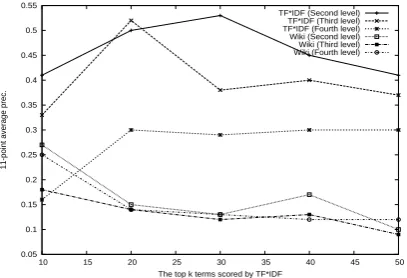
0.05 0.1 0.15 0.2 0.25 0.3 0.35 0.4 0.45 0.5 0.55
10 15 20 25 30 35 40 45 50
11-point average prec.
The top k terms scored by TF*IDF
TF*IDF (Second level) TF*IDF (Third level) TF*IDF (Fourth level) Wiki (Second level) Wiki (Third level) Wiki (Fourth level)
Figure 1: Performance against the topkterms
terms. The results are shown in Table 3. As can be seen clearly from Table 3, the results ob-tained by concepts based method were better than TF∗IDF and Wikipedia in both types of data. The results obtained by concepts based method show that there is no significant difference between two types of data, while the results by Wikipedia go down when we tested data that correct labels do not occur in the documents. This shows that the use of concepts in a dictionary improves overall performance. Table 4 shows a list of top 2 terms identified by concepts based method. Bold font
terms are correctly identified by the method. Ta-ble 4 shows that more than half of the terms are correctly identified in the second and third level of a hierarchy.
We note that we set the number of scored terms to 20. To examine how the number of scored terms affects the overall performance, we per-formed an experiment by varying the values. Fig-ure 1 shows performance plots against the top k terms scored by TF∗IDF. The best performance by both methods was around the top 20 terms scored by TF∗IDF term weighting method. The larger the number of scored terms becomes low precision. This is reasonable because a good label for a clus-ter generally consists of a few words.
4 Conclusions
[image:4.595.83.287.415.554.2]Acknowledgement
The authors would like to thank the referees for their comments on the earlier version of this paper. This work was partially supported by the Telecom-munications Advancement Foundation.
References
D. Camel, E. Yom-Tov, A. Darlow, and d. Pelleg. 2009. What Makes a Query Difficult? In Proc. of the
32rd International ACM SIGIR Conference on Re-search and Development in Information Retrieval,
pages 139–146.
O. S. Chin, N. Kulathuramaiyer, and A. W. Yeo. 2006. Automatic Discovery of Concepts from Text. In
Proc. of the 2006 IEEE/WIC/ACM International Conference on Web Intelligence, pages 1046–1049.
D. R. Cutting, J. O. Pedersen, D. Karger, and J. W. Tukey. 1992. Scatter/ gather: A Cluster-based Ap-proach to Browsing Large Document Collections. In
Proc. of the 15th Annual International ACM SIGIR Conference on Research and Development in Infor-mation Retrieval, pages 318–329.
C. Fellbaum. 1998. An WordNet Electronic Lexical
Database. The MIT Press.
E. Gabrilovich and S. Markovitch. 2007. Computing Semantic Relatedness using Wikipedia-based Ex-plicit Semantic Analysis. In Proc. of the 20th
Inter-national Joint Conference on Artificial Intelligence,
pages 1606–1611.
F. Geraci, M. Pellegrini, m. Maggini, and F. Sebas-tiani. 2007. Cluster Generation and Labeling for Web Snippets: A Fast, Accurate Hierarchical Solu-tion. Internet Mathematics, 3(4):413–443.
S. Kirkpatrick, C. G. Jr., and M. Vecchi. 1983. Optimization by simulated annealing. Science,
220(4598):671–680.
M. Muhr, R. Kern, and M. Granitzer. 2010. Analysis of Structural Relationships for Hierarchical Cluster Labeling. In Proc. of the 33rd International ACM
SIGIR Conference on Research and Development in Information Retrieval, pages 19–23.
R. Nock, P. Vaillant, C. Henry, and F. Nielsen. 2009. Soft Membershipfs for Spectral Clustering with Ap-plication to Premeable Language Distinction.
Pat-tern Recognition, 42:43–53.
S. Osinski and D. Weiss. 2005. A Concept-Driven Algorithm for Clustering Search Results. IEEE
In-telligent Systems, 20(3):48–54.
A. Popescul and L. H. Ungar. 2000. Automatic Label-ing of Document Clusters.
J. Reichardt and S. Bomholdt. 2006. Statistical Me-chanics of Community Detection. PHYSICAL
RE-VIEW E, 74.
J. Reichardt and S. Bornholdt. 2004. Detecting Fuzzy Community Structure in Complex Networks with a Potts Model. PHYSICAL REVIEW LETTERS,
93(21).
RWC. 1998. RWC Text Database. In Real World Computing Partnership.
Z. S. Syed, T. Finin, and A. Joshi. 2008. Wikipedia as an Ontology for Describing Documents. In Proc. of