Large-scale patterns of forest fire occurrence in the conterminous United States, Alaska, and Hawaii, 2014

(1)

Forest Health Monitoring:

National Status, Trends, and Analysis 2015

Editors

Kevin M. Potter

Barbara L. Conkling

United States Department of Agriculture

Forest Service

(2)

41

CHAPTER 3. Large-Scale Patterns of

Forest Fire Occurrence in

the Conterminous United

States, Alaska, and

Hawai‘i, 2014

Kevin M. Potter

INTRODUCTION

F

ree-burning wildland fire has been a frequent

ecological phenomenon on the American landscape, and its expression has changed as new peoples and land uses have become predominant (Pyne 2010). As a pervasive disturbance agent operating at many spatial and temporal scales, wildland fire is a key abiotic factor affecting forest health both positively and negatively. In some ecosystems, wildland fires have been essential for regulating processes that maintain forest health (Lundquist and others 2011). Wildland fire, for example, is an important ecological mechanism that shapes the distributions of species, maintains the structure and function of fire-prone communities, and acts as a significant evolutionary force (Bond and Keeley 2005).

At the same time, wildland fires have created forest health problems in some ecosystems (Edmonds and others 2011). Specifically, fire outside the historic range of frequency and intensity can impose extensive ecological and socioeconomic impacts. Current fire regimes on more than half of the forested area in the conterminous United States have been moderately or significantly altered from historical regimes, potentially altering key ecosystem components such as species composition, structural stage, stand age, canopy closure, and fuel loadings (Schmidt and others 2002). Understanding existing fire regimes is essential to properly assessing the impact of fire on forest health because changes to historical

fire regimes can alter forest developmental patterns, including the establishment, growth, and mortality of trees (Lundquist and others 2011).

As a result of intense suppression efforts during most of the 20th century, the forest area burned annually decreased from approximately 16 million to 20 million ha (40–50 million acres) in the early 1930s to about 2 million ha (5 million acres) in the 1970s (Vinton 2004). In some regions, plant communities have experienced or are undergoing rapid compositional and structural changes as a result of fire suppression (Nowacki and Abrams 2008). At the same time, fires in some regions and ecosystems have become larger, more intense, and more damaging because of the accumulation of fuels as a result of prolonged fire suppression (Pyne 2010). Such large wildland fires also can have long lasting social and economic consequences, which include the loss of human life and property, smoke-related human health impacts, and the economic cost and dangers of fighting the fires themselves (Gill and others 2013, Richardson and others 2012).

(3)

SECTION 1

Chapter 3 Forest Health Monitoring

42

and recurrence could result in decreased forest resilience and persistence (Lundquist and others 2011), and fire regimes altered by global climate change could cause large-scale shifts in vegetation spatial patterns (McKenzie and others 1996).

This chapter presents analyses of fire occurrence data, collected nationally each day by satellite, that map and quantify where fire occurrences have been concentrated spatially across the conterminous United States, Alaska, and Hawai‘i in 2014. It also, within a geographic context, compares 2014 fire occurrences to all the recent years for which such data are available. Quantifying and monitoring such medium-scale patterns of fire occurrence across the United States can help improve the understanding of the ecological and economic impacts of fire as well as the appropriate management and prescribed use of fire. Specifically, large-scale assessments of fire occurrence can help identify areas where specific management activities may be needed, or where research into the ecological and socioeconomic impacts of fires may be required.

METHODS

Data

Annual monitoring and reporting of active wildland fire events using the Moderate

Resolution Imaging Spectroradiometer (MODIS) Active Fire Detections for the United States database (USDA Forest Service 2015) allows

analysts to spatially display and summarize fire occurrences across broad geographic regions (Coulston and others 2005; Potter 2012a, 2012b, 2013a, 2013b, 2014, 2015a, 2015b). A fire occurrence is defined as one daily satellite

detection of wildland fire in a 1-km2 pixel, with

multiple fire occurrences possible on a pixel across multiple days resulting from a single wildland fire lasting multiple days. The data are derived using the MODIS Rapid Response System (Justice and others 2002, 2011) to extract fire location and intensity information from the thermal infrared bands of imagery collected daily by two satellites at a resolution

of 1 km2, with the center of a pixel recorded as

a fire occurrence (USDA Forest Service 2015). The Terra and Aqua satellites’ MODIS sensors identify the presence of a fire at the time of image collection, with Terra observations collected in the morning and Aqua observations collected in the afternoon. The resulting fire occurrence data represent only whether a fire was active because the MODIS data bands do not differentiate between a hot fire in a relatively

small area (0.01 km2, for example) and a cooler

fire over a larger area (1 km2, for example).

(4)

43

be preferable but can be difficult to obtain or may not exist (Tonini and others 2009). For more information about the performance of this product, see Justice and others (2011).

It is important to underscore that estimates of burned area and calculations of MODIS-detected fire occurrences are two different metrics for quantifying fire activity within a given year. Most importantly, the MODIS data contain both spatial and temporal components because persistent fire will be detected repeatedly over

several days on a given 1-km2 pixel. In other

words, a location can be counted as having a fire occurrence multiple times, once for each day a fire is detected at the location. Analyses of the MODIS-detected fire occurrences, therefore,

measure the total number of daily 1-km2

pixels with fire during a year, as opposed to quantifying only the area on which fire occurred at some point during the course of the year.

Analyses

These MODIS products for 2014 were

processed in ArcMap® (ESRI 2012) to determine

number of fire occurrences per 100 km2

(10 000 ha) of forested area for each ecoregion section in the conterminous 48 States (Cleland and others 2007) and Alaska (Nowacki and Brock 1995) and for each of the major islands of Hawai‘i. This forest fire occurrence density measure was calculated after screening out wildland fires on nonforested pixels using a forest cover layer derived from MODIS imagery by the U.S. Forest Service Remote Sensing

Applications Center (RSAC) (USDA Forest Service 2008). The total numbers of forest fire occurrences were also determined separately for the conterminous States, Alaska, and Hawai‘i.

(5)

SECTION 1

Chapter 3 Forest Health Monitoring

44

considered statistically greater than or less than the long-term mean (at p < 0.025 at each tail of the distribution).

Additionally, we used the Spatial Association of Scalable Hexagons (SASH) analytical approach to identify forested areas in the conterminous 48 States with higher-than-expected fire occurrence density in 2014. This method identifies locations where ecological phenomena occur at greater or lower occurrences than expected by random chance and is based on a sampling frame optimized for spatial neighborhood analysis, adjustable to the appropriate spatial resolution, and applicable to multiple data types (Potter and others 2016). Specifically, it consists of dividing an analysis area into scalable equal-area hexagonal cells within which data are aggregated, followed by identifying statistically significant geographic clusters of hexagonal cells within which mean values are greater or less than those expected by chance. To identify these

clusters, we employed a Getis-Ord (G_i*) hot spot

analysis (Getis and Ord 1992) in ArcMap® 10.1

(ESRI 2012).

The spatial units of analysis were 9,810

hexagonal cells, each approximately 834 km2

in area, generated in a lattice across the

conterminous United States using intensification of the Environmental Monitoring and

Assessment Program (EMAP) North American hexagon coordinates (White and others 1992). These coordinates are the foundation of a sampling frame in which a hexagonal lattice was projected onto the conterminous United

States by centering a large base hexagon over the region (Reams and others 2005, White and others 1992). This base hexagon can be subdivided into many smaller hexagons, depending on sampling needs, and serves as the basis of the plot sampling frame for the FIA program (Reams and others 2005). Importantly, the hexagons maintain equal areas across the study region regardless of the degree of intensification of the EMAP hexagon coordinates. In addition, the hexagons are compact and uniform in their distance to the centroids of neighboring hexagons, meaning that a hexagonal lattice has a higher degree of isotropy (uniformity in all directions) than does a square grid (Shima and others 2010). These are convenient and highly useful attributes for spatial neighborhood analyses. These scalable hexagons also are independent of geopolitical and ecological boundaries, avoiding the possibility of different sample units (such as counties, States, or watersheds) encompassing vastly different areas (Potter and others 2016).

We selected hexagons 834 km2 in area because

this is a manageable size for making monitoring and management decisions in nationwide analyses (Potter and others 2016).

Fire occurrence density values for each hexagon were quantified as the number of forest

fire occurrences per 100 km2 of forested area

within the hexagon. The Getis-Ord G_i* statistic

(6)

45

decomposition of a global measure of spatial association into its contributing factors, by location, and is therefore particularly suitable for detecting outlier assemblages of similar conditions (i.e., nonstationarities) in a dataset, such as when spatial clustering is concentrated in one subregion of the data (Anselin 1992).

Briefly, G_i* sums the differences between the

mean values in a local sample, determined in this case by a moving window of each hexagon and its 18 first- and second-order neighbors (the 6 adjacent hexagons and the 12 additional hexagons contiguous to those 6) and the global mean of all the forested hexagonal cells in the

conterminous 48 States. G_i* is standardized

as a z-score with a mean of 0 and a standard deviation of 1, with values > 1.96 representing significant local clustering of higher fire occurrence densities (p < 0.025) and values < -1.96 representing significant clustering of lower fire occurrence densities (p < 0.025) because 95 percent of the observations under a normal distribution should be within

approximately 2 standard deviations of the mean (Laffan 2006). Values between -1.96 and 1.96 have no statistically significant concentration of high or low values; a hexagon and its 18 neighbors, in other words, have a range of both high and low numbers of fire occurrences

per 100 km2 of forested area. It is worth

noting that the threshold values are not exact because the correlation of spatial data violates the assumption of independence required for

statistical significance (Laffan 2006). The Getis-Ord approach does not require that the input data be normally distributed, because the local

G_i* values are computed under a randomization

assumption, with G_i* equating to a standardized

z-score that asymptotically tends to a normal

distribution (Anselin 1992). The z-scores are reliable, even with skewed data, as long as the distance band is large enough to include several neighbors for each feature (ESRI 2012).

RESULTS AND DISCUSSION

(7)

SECTION 1

Chapter 3

0 20,000 40,000 60,000 80,000 100,000 120,000 140,000 160,000

2001 2002 2003 2004 2005 2006 2007 2008 2009 2010 2011 2012 2013 2014

Conterminous States Alaska

Hawai‘i

Total

Forest fire occurrences

Year

Forest Health Monitoring

46

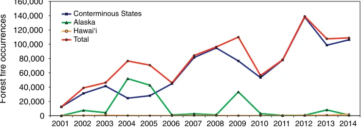
The increase in the total number of fire occurrences across the conterminous United States is generally consistent with the official wildland fire statistics (National Interagency Coordination Center 2015). In 2014, 63,612 wildfires were reported nationally, compared to 47,579 the previous year. The area burned nationally in 2014 (1 455 092 ha) was 53 percent of the 10-year average, with 9 fires exceeding 16 187 ha (11 fewer than in 2013) (National Interagency Coordination Center 2015). The total area burned nationally represented a 17 percent decrease from 2013 (1 748 058 ha) (National Interagency Coordination Center 2014). As noted in Methods section, such estimates of burned

Figure 3.1—Forest fire occurrences detected by Moderate Resolution Imaging Spectroradiometer (MODIS) from 2001 to 2014 for the conterminous United States, Alaska and Hawai‘i, and for the entire Nation combined. (Data source: U.S. Department of Agriculture, Forest Service, Remote Sensing Applications Center, in conjunction with the NASA MODIS Rapid Response group)

area are different metrics for quantifying fire activity than calculations of MODIS-detected fire occurrences, though the two may be correlated.

In 2014, the highest forest fire occurrence densities occurred in northern California, in southern Oregon, in northern Washington, and across parts of the Southeast (fig. 3.2), reflecting the severe to exceptional drought conditions that continued from previous years and extended from the Pacific Coast to the western slope of the Rocky Mountains, and also existed across the southern plains (National Interagency Coordination Center 2015). The forested ecoregion with the highest wildland forest fire occurrence density in 2014

(8)

47

Fire occurrences

per 100 km2_forest

0–1 1.1–3 3.1–6 6.1–12 12.1–24 > 24

Ecoregion section

State

(9)

SECTION 1

Chapter 3 Forest Health Monitoring

48

was section M261A–Klamath Mountains (fig. 3.2) in northern California and southern Oregon. Immediately to the east is M261D– Southern Cascades, with a high fire density of

14.5 per 100 km2 of forest. In these areas, the

lightning-ignited Happy Camp fire complex

burned 542.5 km2, and the July complex

burned 202.5 km2. Fire occurrence density was

20.7 in M242D–Northern Cascades, location of the Carlton complex fire, the largest fire in the history of Washington State, burning

1,036.4 km2. Meanwhile, two ecoregions that

stretch in an arc from southern Mississippi to North Carolina experienced high fire occurrence

densities: 15.9 fires per 100 km2 of forest in

232J–Southern Atlantic Coastal Plains and Flatwoods, and 14.8 fires in 232B–Gulf Coastal Plains and Flatwoods. In central Oklahoma, 255A–Cross Timbers and Prairie had 15.7 fires

per 100 km2 of forest.

Additionally, several ecoregions that contain relatively small amounts of forest (and therefore do not stand out as easily on fig. 3.2) also had high fire occurrence densities in 2014, including 342I–Columbia Basin in central Washington (41.3 fire occurrences per

100 km2 of forest), 251F–Flint Hills in eastern

Kansas (26.4 fire occurrences), and 342H–Blue Mountain Foothills in eastern Oregon (12.1 fire occurrences).

Several ecoregions of the Southeastern United States experienced relatively high fire occurrence densities in 2014 (fig. 3.2). These

encompassed all of the ecoregions of peninsular Florida: 232D–Florida Coastal Lowlands-Gulf,

11.9 fire occurrences per 100 km2 of forest;

232G–Florida Coastal Lowlands-Atlantic, 11.6 fire occurrences; 232K–Florida Coastal Plains Central Highlands, 10.7 fire occurrences; 411A– Everglades, 10.1 fire occurrences; 232L–Gulf Coast Lowlands, 8.2 fire occurrences. Other Southeastern ecoregions with relatively high fire occurrence included the following:

• 232C–Atlantic Coastal Flatwoods (northeastern Florida, eastern Georgia, eastern South Carolina, and southeastern North Carolina), 9.4 fire occurrences; • 232F–Coastal Plains and Flatwoods-Western

Gulf (west-central Louisiana and east-central Texas), 8.0 fire occurrences;

• 231B–Coastal Plains-Middle (central Alabama, northeastern Mississippi, and southwestern Tennessee), 7.8 fire occurrences;

• 231A–Southern Appalachian Piedmont (east-central Alabama, northern Georgia, and northern South Carolina), 7.4 fire occurrences;

• 231G–Arkansas Valley (west-central Arkansas and east-central Oklahoma), 7.6 fire

occurrences; and

• M231A–Ouchita Mountains (west-central Arkansas and southeastern Oklahoma), 7.5 fire occurrences.

(10)

49

occurrences per 100 km2 of forest) to the Sierra

Nevada range of central California (M261E– Sierra Nevada) experienced moderate fire occurrence densities. Farther east, M341A–East Great Basin and Mountains in eastern Nevada (7.2 fire occurrences) and 313D–Painted Desert and M313A–White Mountains-San Francisco Peaks-Mogollon Rim in eastern Arizona (9.1 and 6.1 fire occurrences, respectively) had similarly moderate fire occurrence densities. Fire occurrence densities, meanwhile, were generally low in the Northeastern, Mid-Atlantic, Midwestern, and central Rocky Mountain States (fig. 3.2).

Alaska had warm, dry, and windy conditions in the spring and summer months of 2014, which led to fuels becoming rapidly snow free across the southern two-thirds of the State (National Interagency Coordination Center 2015). Still, Alaska saw a relatively small

number of fires, and all but one ecoregion in the State had low fire occurrence densities (fig. 3.3). The exception was 213B–Cook Inlet Lowlands,

with 3.5 fire occurrences per 100 km2 of forest,

stemming from the human-ignited Funny River fire on the Kenai Peninsula, which burned 79 260 ha in late May and early June and cost $11.4 million to control (National Interagency Coordination Center 2015).

The first half of 2014 was abnormally dry in Hawai‘i (National Interagency Coordination Center 2015), but most forest fire occurrences were associated with the months-long eruption

of Pu‘u ‘Ō‘ō, a vent on the flank of the Kilauea

volcano, which sent a slow moving flow of lava through dense forest near the eastern edge of the Big Island (Miner 2014). As a result, fire occurrence density on the Big Island was 44.1

per 100 km2 of forest (fig. 3.4). Densities on

the other islands were all less than one fire per

100 km2 of forest.

Comparison to Longer Term Trends

Contrasting short-term (1-year) wildland forest fire occurrence densities with longer term trends is possible by comparing these results for each ecoregion section to the first 13 full years of MODIS Active Fire data collection (2001– 2013). In general, most ecoregions within the Northeastern, Midwestern, Mid-Atlantic, and Appalachian regions experienced less than 1

fire per 100 km2 of forest during the multiyear

(11)

SECTION 1

Chapter 3

Fire occurrences per 100 km2_forest

0–1 1.1–3 3.1–6 6.1–12 12.1–24 > 24

Ecoregion section

Forest Health Monitoring

50

(12)

51

Figure 3.4—The number of forest fire occurrences, per 100 km2 (10 000 ha) of forested area, by island in Hawai‘i, for 2014. Forest cover is derived from MODIS imagery by the U.S. Forest Service Remote Sensing Applications Center. (Source of fire data: U.S. Department of Agriculture, Forest Service, Remote Sensing Applications Center, in conjunction with the NASA MODIS Rapid Response group)

Fire occurrences per 100 km2_forest

0–1 1.1–3 3.1–6 6.1–12 12.1–24 > 24

(13)

SECTION 1

Chapter 3 Forest Health Monitoring

52

Oregon, north-central Washington, western Montana, western Utah, northeastern Nevada, central and southeastern Arizona, southwestern New Mexico, and eastern North Carolina (fig. 3.5B). Less variation occurred throughout the Southeast, coastal and eastern Oregon and Washington, the Rocky Mountain States, and northern Minnesota. The lowest levels of variation were apparent throughout most of the Midwest and Northeast.

In 2014, ecoregions in the Pacific Northwest, in the Great Basin, in the Southwest, and across much of the Eastern United States experienced greater fire occurrence densities than normal, compared to the previous 13-year mean and accounting for variability over time, as determined by the calculation of standardized fire occurrence z-scores (fig. 3.5C). These included ecoregions in the Midwest, Mid-Atlantic, and New England States, which had high z-scores despite a relatively low density of fire occurrences in 2014 (fig. 3.2) because these were slightly higher than normal in areas that typically have very little variation over time in fire occurrence density. On the other hand, several of the western and southeastern ecoregions with high z-scores also had very high fire occurrence densities in 2014 (fig. 3.2), including M261A–Klamath Mountains in northwestern California and southwestern Oregon, M242D–Northern Cascades in north-central Washington, 232B–Gulf Coastal Plains and Flatwoods in southern Mississippi and Alabama and northwestern Florida, and 232J– Southern Atlantic Coastal Plains and Flatwoods in central Georgia, central South Carolina, and

south-central North Carolina (fig. 3.2). No ecoregions had lower fire occurrence densities in 2014 compared to the longer term.

In Alaska, meanwhile, the highest mean annual fire occurrence density between 2001 and 2013 occurred in the east-central and central parts of the State (fig. 3.6A) in the 139A– Yukon Flats ecoregion, with moderate mean fire occurrence density in neighboring areas. As expected, many of those same areas experienced the greatest degree of variability over the

13-year period (fig. 3.6B). In 2014, only one ecoregion was outside the range of near-normal fire occurrence density, compared to the mean of the previous 13 years and accounting for variability (fig. 3.6C). This was 213B–Cook Inlet Lowlands, an area with typically very low mean fire occurrence density (fig. 3.6A) and variability (fig. 3.6B) that was the location of the Funny River fire, the third largest wildfire nationally in 2014.

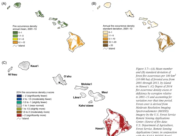
In Hawai‘i, both the mean annual fire occurrence density (fig. 3.7A) and variability (fig. 3.7B) were highest on the Big Island during the 2001–2013 period. The annual

mean was less than 1 fire per 100 km2 of forest

for all islands except the Big Island (8.1) and

Kahoʻolawe (1.9). The annual fire occurrence

standard deviation exceeded 1 for only the Big

Island (11.9), Kahoʻolawe (5.4), and Lānaʻi

(14)

53

0–1 1.1–3 3.1–6 6.1–12 Fire occurrence density annual mean, 2001–13

> 12

Ecoregion section State

< -2 (significantly fewer) -2 to -1.5 (moderately fewer) -1.5 to -1 (slightly fewer) -1 to 1 (near normal) 1 to 1.5 (slightly more) 2014 fire occurrence density z-score

> 2 (significantly more) 1.5 to 2 (moderately more)

0–1 1.1–3 3.1–6 6.1–12 Fire occurrence density annual mean, 2001–13

> 12

0–1 1.1–5 5.1–10 10.1–20

Annual fire occurrence density standard deviation, 2001–13

> 20

0–1 1.1–5 5.1–10 10.1–20

> 20

Figure 3.5—(A) Mean number and (B) standard deviation of forest fire occurrences per 100 km2 (10 000 ha) of forested area from 2001 through 2013, by ecoregion section within the conterminous 48 States. (C) Degree of 2014 fire occurrence density excess or deficiency by ecoregion relative to 2001–13 and accounting for variation over that time period. The dark lines delineate ecoregion sections (Cleland and others 2007). Forest cover is derived from Moderate Resolution Imaging Spectroradiometer (MODIS) imagery by the U.S. Forest Service Remote Sensing Applications Center. (Source of fire data: U.S. Department of Agriculture, Forest Service, Remote Sensing Applications Center, in conjunction with the NASA MODIS Rapid Response group)

(A)

(C)

(15)

SECTION 1

Chapter 3 Forest Health Monitoring

54 (A)

(C)

(B)

Figure 3.6—(A) Mean number and (B) standard deviation of forest fire occurrences per 100 km2 (10 000 ha) of forested area from 2001 through 2013, by ecoregion section in Alaska. (C) Degree of 2014 fire occurrence density excess or deficiency by ecoregion relative to 2001–13 and accounting for variation over that time period. The dark lines delineate ecoregion sections (Nowacki and Brock 1995). Forest cover is derived from Moderate Resolution Imaging Spectroradiometer (MODIS) imagery by the U.S. Forest Service Remote Sensing Applications Center. (Source of fire data: U.S. Department of Agriculture, Forest Service, Remote Sensing Applications Center, in conjunction with the NASA MODIS Rapid Response group)

0–1 1.1–3 3.1–6 6.1–12

Fire occurrence density annual mean, 2001–13

Ecoregion section

0–1 1.1–5 5.1–10 10.1–20

> 20

Ecoregion section

(16)

55 (A)

(C)

(B)

Figure 3.7—(A) Mean number and (B) standard deviation of forest fire occurrences per 100 km2 (10 000 ha) of forested area from 2001 through 2013, by island in Hawai‘i. (C) Degree of 2014 fire occurrence density excess or deficiency by ecoregion relative to 2001–13 and accounting for variation over that time period. Forest cover is derived from Moderate Resolution Imaging Spectroradiometer (MODIS) imagery by the U.S. Forest Service Remote Sensing Applications Center. (Source of fire data: U.S. Department of Agriculture, Forest Service, Remote Sensing Applications Center, in conjunction with the NASA MODIS Rapid Response group)

0–1 1.1–3 3.1–6 6.1–12

Fire occurrence density annual mean, 2001–13

Island

0–1 1.1–5 5.1–10 10.1–20

> 20

Island

(17)

SECTION 1

Chapter 3 Forest Health Monitoring

56 Geographical Hot Spots of Fire

Occurrence Density

Although summarizing fire occurrence data at the ecoregion scale allows for the quantification of fire occurrence density across the country, a geographical hot spot analysis can offer insights into where, statistically, fire occurrences are more concentrated than expected by chance. In 2014, the two geographical hot spots with the highest fire occurrence densities were located in northwestern California/southwestern Oregon and in north-central Washington (fig. 3.8). The larger of these was detected in M261A– Klamath Mountains, the area with the highest wildland forest fire occurrence density in 2014. This hot spot extended, at lower levels of fire occurrence density, into M261D–Southern Cascades and M221G–Modoc Plateau. The other hot spot of very high fire occurrence density was in M242D–Northern Cascades, extending with lower fire occurrence density into the neighboring M333A–Okanogan Highland.

Several hot spots of moderate to high fire density were scattered elsewhere across the Western United States (fig. 3.8), including in the following regions:

• Central Oregon (M332G–Blue Mountains, M242C–Eastern Cascades, and M242B– Western Cascades),

• West-central Idaho and northeastern Oregon (M332A–Idaho Batholith and M332G– Blue Mountains),

• East-central Nevada (M341A–East Great Basin and Mountains),

• East-central Arizona (M313A–White Mountains-San Francisco Peaks-Mogollon Rim and 313C–Tonto Transition),

• Southern California (261B–Southern California Coast and M262B–Southern California Mountain and Valley), and

• Central California (M261E–Sierra Nevada and M261F–Sierra Nevada Foothills).

The geographic clustering analysis detected a large hot spot in the Southeast, extending across four States and having its high fire density core in ecoregion 232B–Gulf Coast Plains and Flatwoods in southwestern Georgia and north-central Florida (fig. 3.8). Within the East, other hot spots of high fire occurrence density were located in southern Florida (232D–Florida Coastal Lowlands-Gulf and 411A–Everglades), southern Louisiana (234C–Atchafalaya and Red River Alluvial Plains), and southeastern Kansas and northeastern Oklahoma (255A– Cross Timbers and Prairie). The Southeastern United States was the region with the greatest area burned in 2014 (National Interagency Coordination Center 2015), but these were mostly small, short-duration fires occurring in the spring or autumn.

CONCLUSION

The results of these geographic analyses are intended to offer insights into where fire occurrences have been concentrated spatially in a given year and compared to previous years, but are not intended to quantify the severity of a given fire season. Given the limits of MODIS

(18)

57

2.01–6 (Clustered, moderate density)

6.01–12 (Clustered, high density) 12.01–24 (Clustered, very high density) Clustering and degree

of fire occurrence density ≤ 2 (Not clustered)

> 24 (Clustered, extremely high density)

State

Ecoregion section

(19)

SECTION 1

Chapter 3 Forest Health Monitoring

58

data, these products also may underrepresent the number of fire occurrences in some ecosystems where small and low-intensity fires are common. These products can also have commission errors. However, these high temporal fidelity products currently offer the best means for daily monitoring of wildfire impacts. Ecological and forest health impacts relating to fire and other abiotic disturbances are scale-dependent properties, which in turn are affected by management objectives (Lundquist and others 2011). Information about the concentration of fire occurrences may help pinpoint areas of concern for aiding management activities and for investigations into the ecological and socioeconomic impacts of wildland forest fire potentially outside the range of historic frequency.

LITERATURE CITED

Anselin, L. 1992. Spatial data analysis with GIS: an introduction to application in the social sciences. Tech. Rep. 92-10. Santa Barbara, CA: National Center for Geographic Information and Analysis. 53 p.

Barbour, M.G.; Burk, J.H.; Pitts, W.D. [and others]. 1999. Terrestrial plant ecology. Menlo Park, CA: Addison Wesley Longman, Inc. 649 p.

Bond, W.J.; Keeley, J.E. 2005. Fire as a global “herbivore”: the ecology and evolution of flammable ecosystems. Trends in Ecology & Evolution. 20(7): 387–394. Brooks, M.L.; D’Antonio, C.M.; Richardson, D.M. [and

others]. 2004. Effects of invasive alien plants on fire regimes. BioScience. 54(7): 677–688.

Cleland, D.T.; Freeouf, J.A.; Keys, J.E.; [and others]. 2007. Ecological subregions: sections and subsections for the conterminous United States. In: Sloan, A.M., tech. ed. Washington, DC: U.S. Department of Agriculture, Forest Service. Gen. Tech. Rep. WO-76D. [Map, presentation scale 1:3,500,000; colored]. Also on CD-ROM as a GIS coverage in ArcINFO format.

Coulston, J.W.; Ambrose, M.J.; Riitters, K.H.; Conkling, B.L. 2005. Forest Health Monitoring 2004 national technical report. Gen. Tech. Rep. SRS-90. Asheville, NC: U.S. Department of Agriculture, Forest Service, Southern Research Station. 81 p.

Edmonds, R.L.; Agee, J.K.; Gara, R.I. 2011. Forest health and protection. Long Grove, IL: Waveland Press, Inc. 667 p.

ESRI. 2012. ArcMap® 10.1. Redlands, CA: Environmental

Systems Research Institute.

Getis, A.; Ord, J.K. 1992. The analysis of spatial association by use of distance statistics. Geographical Analysis. 24(3): 189–206.

Gill, A.M.; Stephens, S.L.; Cary, G.J. 2013. The

worldwide “wildfire” problem. Ecological Applications. 23(2): 438– 454.

Hawbaker, T.J.; Radeloff, V.C.; Syphard, A.D. [and others]. 2008. Detection rates of the MODIS active fire product. Remote Sensing of Environment. 112: 2656–2664. Justice, C.O.; Giglio, L.; Korontzi, S. [and others]. 2002. The

MODIS fire products. Remote Sensing of Environment. 83(1–2): 244–262.

Justice, C.O.; Giglio, L.; Roy, D. [and others]. 2011. MODIS-derived global fire products. In: Ramachandran, B.; Justice, C.O.; Abrams, M.J., eds. Land remote sensing and global environmental change: NASA’s earth observing system and the science of ASTER and MODIS. New York: Springer: 661–679.

Laffan, S.W. 2006. Assessing regional scale weed

distributions, with an Australian example using Nassella

trichotoma. Weed Research. 46(3): 194–206.

Lundquist, J.E.; Camp, A.E.; Tyrrell, M.L. [and others]. 2011. Earth, wind and fire: abiotic factors and the impacts of global environmental change on forest health. In: Castello, J.D.; Teale, S.A., eds. Forest health: an integrated perspective. New York: Cambridge University Press: 195–243.

(20)

59

Miner, M. 2014. Kilauea Volcano lava flow approaching homes in Hawai‘i Island’s Puna district. Hawaii Magazine. http://www.hawaiimagazine.com/blogs/hawaii_

today/2014/9/12/kilauea_volcano_lava_flow_Puna_Big_ Island. [Date accessed: August 11, 2015].

National Interagency Coordination Center. 2014. Wildland fire summary and statistics annual report: 2013. http:// www.predictiveservices.nifc.gov/intelligence/2013_ Statssumm/intro_summary13.pdf. [Date accessed: May 28, 2014].

National Interagency Coordination Center. 2015. Wildland fire summary and statistics annual report: 2015. http:// www.predictiveservices.nifc.gov/intelligence/2014_ Statssumm/intro_summary14.pdf. [Date accessed: May 11, 2015].

Nowacki, G.J.; Abrams, M.D. 2008. The demise of fire and “mesophication” of forests in the Eastern United States. BioScience. 58(2): 123–138.

Nowacki, G.; Brock, T. 1995. Ecoregions and subregions of Alaska [EcoMap]. Version 2.0. Juneau, AK: U.S. Department of Agriculture, Forest Service, Alaska Region. [Map, presentation scale 1:5,000,000; colored].

Potter, K.M. 2012a. Large-scale patterns of forest fire occurrence in the conterminous United States and Alaska, 2005–07. In: Potter, K.M.; Conkling, B.L., eds. Forest Health Monitoring 2008 national technical report. Gen. Tech. Rep. SRS-158. Asheville, NC: U.S. Department of Agriculture, Forest Service, Southern Research Station: 73–83.

Potter, K.M. 2012b. Large-scale patterns of forest fire occurrence in the conterminous United States and Alaska, 2001-08. In: Potter, K.M.; Conkling, B.L., eds. Forest health monitoring 2009 national rechnical report. Gen. Tech. Rep. SRS-167. Asheville, NC: U.S. Department of Agriculture, Forest Service, Southern Research Station: 151-161.

Potter, K.M. 2013a. Large-scale patterns of forest fire occurrence in the conterminous United States and Alaska, 2009. In: Potter, K.M.; Conkling, B.L., eds. Forest Health Monitoring: national status, trends and analysis 2010. Gen. Tech. Rep. SRS-176. Asheville, NC: U.S. Department of Agriculture, Forest Service, Southern Research Station: 31–39.

Potter, K.M. 2013b. Large-scale patterns of forest fire occurrence in the conterminous United States and Alaska, 2010. In: Potter, K.M.; Conkling, B.L., eds. Forest Health Monitoring: national status, trends and analysis 2011. Gen. Tech. Rep. SRS-185. Asheville, NC: U.S. Department of Agriculture, Forest Service, Southern Research Station: 29–40.

Potter, K.M. 2014. Large-scale patterns of forest fire occurrence in the conterminous United States and Alaska, 2011. In: Potter, K.M.; Conkling, B.L., eds. Forest Health Monitoring: national status, trends and analysis 2012. Gen. Tech. Rep. SRS-198. Asheville, NC: U.S. Department of Agriculture, Forest Service, Southern Research Station: 35–48.

Potter, K.M. 2015a. Large-scale patterns of forest fire occurrence in the conterminous United States and Alaska, 2012. In: Potter, K. M.; Conkling, B. L., ed. Forest Health Monitoring: national status, trends, and analysis 2013. Gen. Tech. Rep. SRS-207. Asheville, North Carolina: U.S. Department of Agriculture, Forest Service, Southern Research Station: 37–53.

Potter, K.M. 2015b. Large-scale patterns of forest fire occurrence in the conterminous United States and Alaska, 2013. In: Potter, K. M.; Conkling, B. L., ed. Forest Health Monitoring: national status, trends, and analysis 2014. Gen. Tech. Rep. SRS-209. Asheville, North Carolina: U.S. Department of Agriculture, Forest Service, Southern Research Station: 39–55.

Potter, K.M.; Koch, F.H.; Oswalt, C.M.; Iannone, B.V. 2016. Data, data everywhere: Detecting spatial patterns in fine-scale ecological information collected across a continent. Landscape Ecology. 31(1): 67–84.

Pyne, S.J. 2010. America’s fires: a historical context for policy and practice. Durham, NC: Forest History Society. 91 p. Reams, G.A.; Smith, W.D.; Hansen, M.H. [and others]. 2005.

(21)

SECTION 1

Chapter 3 Forest Health Monitoring

60

Richardson, L.A.; Champ, P.A.; Loomis, J.B. 2012. The hidden cost of wildfires: economic valuation of health effects of wildfire smoke exposure in southern California. Journal of Forest Economics. 18(1): 14–35.

Schmidt, K.M.; Menakis, J.P.; Hardy, C.C. [and others]. 2002. Development of coarse-scale spatial data for wildland fire and fuel management. Gen. Tech. Rep. RMRS-GTR-87. Fort Collins, CO: U.S. Department of Agriculture, Forest Service, Rocky Mountain Research Station. 41 p. Shima T.; Sugimoto S.; Okutomi, M. 2010. Comparison of

image alignment on hexagonal and square lattices. 2010 IEEE International Conference on Image Processing: 141–144. DOI:10.1109/icip.2010.5654351.

Tonini, M.; Tuia, D.; Ratle, F. 2009. Detection of clusters using space-time scan statistics. International Journal of Wildland Fire. 18(7): 830–836.

U.S. Department of Agriculture (USDA) Forest Service. 2008. National forest type data development. http://svinetfc4. fs.fed.us/rastergateway/forest_type/. [Date accessed: May 13, 2008].

U.S. Department of Agriculture (USDA) Forest Service. 2015. MODIS active fire mapping program: fire detection GIS data. http://activefiremaps.fs.fed.us/gisdata.php. [Date accessed: February 13, 2015].

Vinton, J.V., ed. 2004. Wildfires: issues and consequences. Hauppauge, NY: Nova Science Publishers, Inc. 127 p. White, D.; Kimerling, A.J.; Overton, W.S. 1992. Cartographic