Genomic Model with Correlation Between Additive and Dominance Effects

| GENOMIC SELECTION

Genomic Model with Correlation Between Additive

and Dominance Effects

Tao Xiang,*,‡,§,1_{Ole Fredslund Christensen,}§_{Zulma Gladis Vitezica,** and Andres Legarra}‡ *Key Laboratory of Agricultural Animal Genetics, Breeding and Reproduction of Ministry of Education and Key Laboratory of Swine Genetics and Breeding of Ministry of Agriculture, College of Animal Science and Technology, Huazhong Agricultural University, Wuhan 430070, P. R. China,‡INRA, UMR 1388 GenPhySE, F-31326 Castanet-Tolosan, France,§Center for Quantitative Genetics and Genomics, Department of Molecular Biology and Genetics, Aarhus University, DK-8830 Tjele, Denmark, and **Université de Toulouse, UMR 1388 GenPhySE, F-31326 Castanet-Tolosan, France ORCID ID: 0000-0001-8893-7620 (A.L.)

ABSTRACT Dominance genetic effects are rarely included in pedigree-based genetic evaluation. With the availability of single nucleotide polymorphism markers and the development of genomic evaluation, estimates of dominance genetic effects have become feasible using genomic best linear unbiased prediction (GBLUP). Usually, studies involving additive and dominance genetic effects ignore possible relationships between them. It has been often suggested that the magnitude of functional additive and dominance effects at the quantitative trait loci are related, but there is no existing GBLUP-like approach accounting for such correlation. Wellmann and Bennewitz (2012) showed two ways of considering directional relationships between additive and dominance effects, which they estimated in a Bayesian framework. However, these relationships cannot be fitted at the level of individuals instead of loci in a mixed model, and are not compatible with standard animal or plant breeding software. This comes from a fundamental ambiguity in assigning the reference allele at a given locus. We show that, if there has been selection, assigning the most frequent as the reference allele orients the correlation between functional additive and dominance effects. As a conse-quence, the most frequent reference allele is expected to have a positive value. We also demonstrate that selection creates negative covariance between genotypic additive and dominance genetic values. For parameter estimation, it is possible to use a combined additive and dominance relationship matrix computed from marker genotypes, and to use standard restricted maximum likelihood algorithms based on an equivalent model. Through a simulation study, we show that such correlations can easily be estimated by mixed model software and that the accuracy of prediction for genetic values is slightly improved if such correlations are used in GBLUP. However, a model assuming uncorrelated effects and fitting orthogonal breeding values and dominant deviations per-formed similarly for prediction.

KEYWORDSgenomic model; additive genetic effects; dominance genetic effects; correlation; shared data resource; GenPred; Genomic Selection

F

ROM quantitative genetics theory, statistical additive ge-netic values (also called breeding values) of individuals are obtained from average allele substitution effectsðaÞ;which are functions of functional additive and dominant gene/ marker effects ða and dÞ (Falconer and Mackay 1996). Dominance deviations are differences between genotypic

val-ues and breeding valval-ues, and only include a part of the dom-inant effects of the genes/markers (Falconer and Mackay 1996). Additive genetic varianceð2pqa2_{Þincludes variation}

due to the functional additive and dominant effects, and dominance genetic varianceðð2pqdÞ2Þinvolves only the func-tional dominant effects.

The inclusion of dominance in genomic evaluation models has been proposed by several authors (Suet al.2012; Vitezica et al.2013, 2016; Ertlet al.2014; Muñozet al.2014; Aliloo et al.2016, 2017; Xianget al.2016). In those studies, addi-tive and dominant marker effectsða and dÞ are considered uncorrelated. However, QTL analyses show that the magni-tudes of these effects are dependent (e.g., Bennewitz and Meuwissen 2010).

Copyright © 2018 by the Genetics Society of America doi:https://doi.org/10.1534/genetics.118.301015

Manuscript received April 7, 2018; accepted for publication May 8, 2018; published Early Online May 9, 2018.

Supplemental material available at Figshare: https://doi.org/10.25386/genetics. 6111068.

In the genomic era, the relationship between magnitudes of additive and dominant gene/marker effects has scarcely been modeled (Wellmann and Bennewitz 2011, 2012; Bennewitzet al. 2017). Wellmann and Bennewitz (2011) reviewed evidence for association of magnitudes of additive and dominant effects across QTL. These magnitudes have been shown to be related through the dominance coeffi -cients d¼d=jaj: QTL with large absolute additive effect are likely to be associated with large dominance coeffi -cients, while small additive effects tend to be associated with small dominance coefficients (Caballero and Keightley 1994). These results suggest that across QTL loci it is pos-sible to construct joint distributions of additive and domi-nant effects. Wellmann and Bennewitz (2012) suggested a general hierarchical Bayesian model where absolute addi-tive QTL effects and dominance coefficients were assumed to be dependent withcorðjaj;dÞ.0:

Recently, the dependencies between additive and dom-inant gene effects were considered in a Bayesian model for association analysis (Bennewitzet al.2017). For geno-mic prediction, methods commonly used are linear mixed models and best linear unbiased prediction (BLUP), i.e., genomic BLUP (GBLUP) methods (Suet al.2012; Vitezica et al. 2013). In these models, the relationship between additive and dominant marker effects is ignored. Examin-ing the relationship between a and d and including it in such genomic models could improve the accuracy of predictions.

Even though Bayesian models can take into account the dependencies between additive and dominant gene effects, their implementation by Markov Chain Monte Carlo meth-ods is not straightforward. These models need customary implementations and would be computationally slow for large data sets. In addition, if the relationship between functional additive and dominant marker effects cannot be described as covariance structure of additive and dom-inance effects on individuals, then the standard mixed model animal breeding software,e.g., DMU (Madsen and Jensen 2013), BLUPf90 family (Misztal et al. 2002), or ASREML (Gilmouret al.2009), cannot be used for estimat-ing such relationships.

In this study, we present a novel method to quantify the importance of the relationship between additive and dom-inant effects of QTL using a GBLUP-like method. This method relies on the fact that allele substitution effects contain functional additive and dominant effects that, after phenotypic selection, tend to offset each other. Our ap-proach is based onfixing the most frequent allele as the reference allele. By simulation, we evaluate the benefit of accounting for this relationship (betweena and d) ex-plicitly in the genomic model for genetic parameter esti-mation and the prediction of genetic values, comparing it with the model ignoring the relationship betweena and d; and with the classical orthogonal model based on breed-ing values and dominance deviations (Vitezica et al. 2013).

Materials and Methods

Theory

Consider a quantitative trait that is determined by biallelic quantitative trait loci. For each locus, let the midpoint of the genotypic values of the two homozygotes be the origin (0). Relative to this origin, the genotypic value of a ho-mozygote is defined as eitheraor2a;and the genotypic value of the heterozygote is defined as d, which is the amount the heterozygote deviates from the origin. Note that the functional valueacan be either positive or neg-ative (a point that is rarely explicit in many textbooks), and the magnitude of the difference between the two ho-mozygotes is therefore the absolute value j2aj. For many traits and species, an advantage of heterozygosity is ob-served, known as heterosis or the related phenomenon inbreeding depression (i.e., Lynch and Walsh 1998, chap-ter 10). This phenomenon is typically modeled as a regres-sion of the phenotype on the degree of heterozygosity, for which several metrics exist (i.e., Silióet al.2016; Xianget al. 2016).

Using a genotypic model (i.e., Su et al.2012; Vitezica et al.2016) for additive and dominant genotypic effectsu

and v on individuals we use the notation u¼Za and

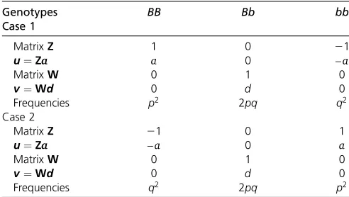
v¼Wd; respectively, where aanddare vectors of func-tional additive and dominant QTL effects across individu-als, respectively, andZandWare the respective incidence matrices. Considering one QTL, the matrixWhas entries 0, 1, and 0 for genotypesBB,Bb, andbb, respectively. For the matrixZ;there are two ways of coding genotypes depend-ing on the selected reference allele: if allele B is the se-lected reference allele, then matrix Z has entries 1, 0, and 21 for BB,Bb, and bb, respectively (case 1 in Table 1); if allelebis selected to be the reference allele, matrixZ

is coded as 21, 0, and 1 for genotypesBB, Bb, and bb, respectively (case 2 in Table 1). Thus, in case 1, additive genotypic effects u forBB, Bb, and bb are a;0; and2a; respectively, and in case 2, additive genotypic effectsufor BB,Bb, andbbare2a;0;anda;respectively. The dominant genotypic effectsvare always 0;d;and 0 for genotypesBB, Bb, and bb, respectively. These two cases can be found in Table 1.

Phenotypic (directional) selection, either artificial by breed-ing or natural, operates to change the phenotype in a desired direction; throughout this paper we will use the shorter term “selection”for this, and without loss of generality we will as-sume that the direction of selection is upwards. Selection acts mainly on the statistical additive component of genetic values. Thus, considering a segregating QTL, then selection will act on the allele substitution effect

a¼aþ ð122pÞd:

Thus, if there is selection, it is expected that no segregating QTL will have a very large allele substitution effect after some generations of selection, leading to:

a¼aþ ð122pÞd¼e (1)

whereeis small. From this we can derivea:¼ ð2p21Þdþe; and we see thataandð2p21Þdwill tend to have the same sign and magnitudes that are positively associated. At this point, a refers to an arbitrary allele (B or b) whose fre-quency isp;and both aandd can have positive or nega-tive values. The allelic frequency 0,p,1 and therefore 2p21 can also be positive or negative, and we see from a¼ ð2p21Þdþethat there is no association between sign ofaand signs of eitherð2p21Þord:We will call this“ ran-dom allele coding”(RAC).

An alternative presentation of the same idea is consider-ing allelic frequency at equilibrium after several rounds of selection (Crow and Kimura 2009; Charlesworth and Charlesworth 2010). If the fitnesses at the locus are2a; d, anda (the actual values are functions ofa andd that depend on the selection intensity and the part of genetic vari-ance explained by the locus; Charlesworth and Charlesworth 2010, box 3.7), the frequency at equilibrium isp¼0:5þa=2d; which is a rewriting of Equation (1). Thus, 2p21 anda=dhave the same sign.

Consider now the equilibria. If2jaj,d,jaj;loci tend to fixation toward the favorable homozygote. Ifjdj.jaj (over-dominance or under(over-dominance), equilibria arestablewhen d.jaj(overdominance) and there is maintenance of poly-morphisms in the population, but ifd, 2jaj (underdomi-nance) the equilibrium is unstable and any random event will lead loci tofixation (Crow and Kimura 2009; Charlesworth

and Charlesworth 2010). Thus, selection tends to maintain primarily overdominant alleles and therefore, after a selec-tion process, it is expected thatd.0 (either across segre-gating loci or across repeated evolutionary histories of the same locus).

Now we extend the reasoning to several loci with random effects drawn from some distributions. Consider a collection of loci with elementsai;di, andpi;respectively, andðai;di;piÞ; i¼1;. . .;Nare treated independent and identically distrib-uted across loci. We can formalize the abovefinding to the co-variance between a andð2p21Þd ascovðai;ð2pi21ÞdiÞ.0; with EðaiÞ ¼0 and EðdiÞ.0: For RAC we see from ai¼ ð2pi21Þdiþei that there is no association between sign ofaiand signs of eitherð2pi21Þordi:This we formal-ize as:

covðai;diÞ ¼EðaidiÞ2EðaiÞEðdiÞ

¼E2pi21

diþei

di

20

E

ð2pi21Þd2i

¼0 (2)

The last identity holds because 2pi21 has zero mean due to pihaving a symmetric distribution with mean 0.5 [could be a uniform distribution between 0 and 1 or a U-shaped distribu-tion (Hillet al.2008)] for the RAC, and assuming that con-ditional mean and variance ofdido not depend onpi:This means that postulating in the model a covariance betweena anddhas no meaning (or interest) because this covariance is 0 under these assumptions.

However, returning to the one-locus case, we can mea-sure its allelic frequency p; and we can arbitrarily fix the most frequent allele as the reference allele such that p.0:5:We will indicate this hereinafter as“major allele coding”(MAC). In such case, allelic frequencypis denoted as pMAC_(p¼pMAC_{.0:5). Additive effect a still} refers to the allele whose frequency is p (actually now ispMAC_{) and is denoted asa}MAC_:Still,aMAC_{can have} pos-itive or negative values. The functional dominance effect d is invariant to the reference allele. Equation (1) still holds:

aMAC¼aMACþ122pMACd¼e:

By the restriction pMAC_{.0:5; the term 2p}MAC_{21 in} aMAC _ð2pMAC_{21Þdþe becomes strictly positive and we} see thataMAC_{anddwill tend to have the same sign. In} addi-tion, because EðdÞ.0 andeis small, then it turns out that EðaMAC_Þ.0:

Consider now the covariance, across several loci, between functional additive (aMAC_{) and dominant (d) effects; then we} formalize the abovefinding to

covaMAC_i ;di

¼cov

ðð

2pMAC_i 21

Þ

diþe;di

Þ

cov

ðð

2pMAC_i 21

Þ

þdi;di

Þ

.0 (3)

where the last inequality follows from

Table 1 Different ways of allele coding for incidence matrices for additive and dominance effects

Genotypes BB Bb bb

Case 1

MatrixZ 1 0 21

u¼Za a 0 –a

MatrixW 0 1 0

v¼Wd 0 d 0

Frequencies p2 _{2pq q}2

Case 2

MatrixZ 21 0 1

u¼Za –a 0 a

MatrixW 0 1 0

v¼Wd 0 d 0

Frequencies q2 _{2pq p}2

cov

ðð

2pMAC

i 21

Þ

di;di

Þ

¼E

ð

cov

ðð

2pMAC_i 21

Þ

di;dijpMACi

ÞÞ

þcov

ð

E

ðð

2pMAC_i 21

Þ

dijpMACi

Þ;

E

ð

dijpMACi

ÞÞ;

where the first term equalsEðð2pMAC

i 21ÞvarðdijpMACi ÞÞ.0; and the second term is zero sinceEðdijpiÞ ¼EðdiÞfor segre-gating loci. If the conditional variance ofdiis not depending onpMAC

i ;thenðð2p MAC

i 21Þdi;diÞ ¼VarðdiÞEð2pMACi 21Þwhere both terms are larger than zero.

Thus, we have shown that, by a careful coding of the model, it is possible to express anafter selectiondependency between functional additive and dominance effects at bial-lelic QTL as a covariance.

So far, we did not consider the dominant coefficientd:If, across loci, there is a biological relationship between the magnitudes of a and d (e.g., Bennewitz and Meuwissen 2010), this mechanism will reinforce the previously men-tioned dependency between functional additive and domi-nance effects. In Appendix A, we consider di¼dijaij; and we argue that it often holds that covðai;diÞ.0 when covðdi;jaijÞ.0 [BayesD3model in Wellmann and Bennewitz (2012)] and covðai;diÞ ¼0 when covðdi;jaijÞ ¼0 [BayesD2 model in Wellmann and Bennewitz (2012)].

Covariance between genotypic additive and dominant effects

In Hardy–Weinberg equilibrium (see Table 1), the covariance between genotypic additive effectsujand dominance effects vj(for a random individual jdrawn from a population) for one QTL can be derived as:

covðuj;vjÞ ¼EðujvjÞ2EðujÞEðvjÞ;

where the expectations can be computed from expectations of conditional expectationsEðujvjja;d;pÞ ¼0 (because the cross product is always zero across the three possible genotypes), Eðujja;d;pÞ ¼ ð2p21Þa;andEðvjja;d;pÞ ¼2pqd;respectively. Therefore,

covðuj;vjÞ ¼ 2Eðð2p21ÞaÞEð2pqdÞ:

As we have already noted, EðdÞ.0 (there will be ten-dency that only overdominant mutations eventually re-main in heterozygous state) and therefore the term Eð2pqdÞis always positive, irrelevant of the coding. When coding genotypes as in the RAC, EðpÞ ¼0:5 and thus EðujÞ ¼Eðð2p21ÞaÞ ¼0. Therefore, covðuj;vjÞ ¼0 holds for RAC. When coding genotypes as in the MAC, Eð2pMAC_{21Þ.0;and there will be a tendency that a}MAC and d have the same sign [see Equation (2)], so that EðaMAC_{Þ.0:In other words, after long-term selection there} will be a tendency that the allele with the positive effect will be most frequent, and henceaMACis positive. To conclude, there will be tendency that both aMAC _{and d are positive.}

Therefore, Eðð2pMAC_21ÞaMAC_{Þ and Eð2pqdÞare both} posi-tive, and hence for the MAC coding

covðuj;vjÞ¼2E

2pMAC21aMACE2pMACqMACd,0 (4)

The intuition behind this is that after long-term selection, individual genotypic additive and dominance effects tend to offset each other in polymorphic loci (otherwise there would befixation).

The expression in Equation (4) extends, assuming linkage equi-librium, tocovðuj;vjÞ ¼ 2

P

Eðð2pMAC

i 21ÞaMACi ÞEð2piqidiÞ,0 for the case of multiple QTL.

For a statistical analysis based on mixed models and

genomic data, the assumption is Var

a d

¼

s2a sad

sad s2d

;

and matricesZandWare known. From theabeing small prop-erty, we have that signs ofaanddare uncorrelated for RAC but positively correlated for MAC. Therefore, we obtainsad¼0 for RAC [Equation (2)] andsad.0 for MAC [Equation (3)].

Variance component estimation

According to the theory sketched before, the variance– covariance structure between genotypic additive and domi-nant effects is:

var

u v

¼var

Za Wd

¼var

Z 0

0 W

a d

¼

Z 0

0 W

var

a d

Z 0

0 W

9

¼

Z 0

0 W

Is2a Isad

Isad Is2d

! Z9 0

0 W9

¼ ZZ9s2a ZW9sad

WZ9sad WW9s2d

! ;

(5)

whereZandWcontain genotypic codings,aanddare addi-tive and dominant SNP effects,s2

ais the additive variance for SNP effects,s2

dis the dominance variance for SNP effects, and

sad is covariance between additive and dominance SNP ef-fects. For different analyses, elements in matrix Z will be coded using RAC (the reference allele is chosen at random for each locus) or using MAC (the reference allele is the most frequent for each locus).

This (co)variance structure in Equation (5) cannot befit in usual BLUP or restricted maximum likelihood (REML) soft-ware directly, because the covariance matrix is not factorizable as a Kronecker product of a relationship structure times a covariance matrix. A solution for this issue is to use an equivalent model with two additional unknown random ef-fects u* and v* (Fernándezet al.2017). Letu*¼Waand

v*¼Zd; these effects have no biological meaningper se. The variance structures foru* andv* arevarðu*Þ ¼WW9s2

aand varðv*Þ ¼ZZ9s2

whereKis an additive-dominance unscaled relationship

matrix

ZZ9 ZW9 WZ9 WW9

; K0 is a covariance matrix

s2

a sad

sad s2d

that associates to SNP effects. Equation (6)

is a typical correlated random effects structure, and such structures can befit using mixed model software.

Nevertheless, variance components inK0are associated to

the scale of SNP effects. To adjust variance components in the K0matrix to be associated to the scale of individuals, similar

to Vitezicaet al.(2016) and Xianget al.(2016), a genomic relationship matrix G¼K=ftrðKÞg=2nis introduced, where trðKÞis the trace of the relationship matrixKand 2nis twice the number of individuals involved in the matrix K: The ftrðKÞg=2n is the average of the diagonal elements in the relationship matrix K:Let a constantk¼ ftrðKÞg=2n;then

matrixG¼K=k¼

ZZ9=k ZW9=k

WZ9=k WW9=k

. Then, the Equation

(6) will change to:

var 0 B B B @ u u* v* v 1 C C C

A¼K05K¼K05ðG3kÞ

¼ ks2a ksad

ksad ks2d

! 5G

¼ s*2A s*AD

s*AD s*2D

! 5

ZZ9=k ZW9=k

WZ9=k WW9=k

;

(7)

where s*2

A; s*2D and s*AD are estimated genotypic additive variance, genotypic dominance variance, and covariance between genotypic additive and dominance effects at the level of individuals, and these can be estimated using REML implemented in standard animal breeding software.

Still, these estimated variance components cannot be inter-preted as the genetic variances in the population (Legarra 2016). The estimated variance components in Equation (7) should be scaled to the expected variance components of a population as in Legarra (2016) (see Appendix B), as follows:

s2u¼DZZ9=ks*2A ; s

2

v ¼DWW9=ks*2D; su;v¼DZW9=ks*AD;

(8)

where s2

u is the expected genotypic additive variance,s2v is the expected genotypic dominance variance,su;vis the covari-ance between expected genotypic additive and domincovari-ance effects, and statistics DM¼meanðdiagðMÞÞ2meanðMÞ for

M¼ZZ9=k;ZW9=k;WW9=k; respectively. Thus, the total genetic variance is s2ðuþvÞ¼s2uþs2vþ2su;v ¼DZZ9=ks*2Aþ DWW9=ks*2D þ2DZW9=ks*AD; and the expected correlation be-tween genotypic additive effectsuand genotypic dominance effectsvis:

ru;v¼ su;v

susv¼

DZW9=ks*AD

ffiffiffiffiffiffiffiffiffiffiffiffiffiffiffiffiffiffiffiffiffiffiffiffiffiffiffiffiffiffiffiffiffiffiffiffiffiffiffiffiffi

DZZ9=ks*2A DWW9=ks*2D

q ; (9)

Replacing DZW9=k in the formula above by its expectation 2Pið2pi21Þð2piqiÞ=k(see Appendix B), which is negative, and using Equations (3) and (7) to see that s*AD.0; we obtain thatru;v is negative, as also shown in Equation (4).

We derived formulae that can be used to estimate the co-variance between genotypic additive and dominant effects. Based on this, four hypothesis can be proposed: (1) association between additive and dominant effects is captured in genomic model by a covariance if the MAC is used, but cannot be captured if the RAC is used; (2) based on Equation (9), the covariancesu;vis negative when the absolute additive effects and dominance coefficients of QTL are positively correlated [e.g.,BayesD3in Wellmann and Ben-newitz (2012)]; (3) a long-term directional selection is a possible cause forsu;v different from 0; and (4) the predictive ability of a var 0 B B @ u u* v_* v 1 C C A¼var

0 B B @ Za Wa Zd Wd 1 C C A¼var

2 6 6 4 0 B B @

Z 0 0 0

0 W 0 0

0 0 Z 0

0 0 0 W

1 C C A 0 B B @ a a d d 1 C C A 3 7 7 5 ¼ 0 B B @

Z 0 0 0

0 W 0 0

0 0 Z 0

0 0 0 W

1 C C A 0 B B @

Is2a Is2a Isad Isad

Is2a Is2a Isad Isad

Isad Isad Is2d Is2d

Isad Isad Is2d Is2d

1 C C A 0 B B @

Z9 0 0 0

0 W9 0 0

0 0 Z9 0

0 0 0 W9

1 C C A ¼ 0 B B @

ZZ9s2a ZW9sa2 ZZ9sad ZW9sad

WZ9s2a WW9sa2 WZ9sad WW9sad

ZZ9sad ZW9sad ZZ9s2d ZW9s2d

WZ9sad WW9sad WZ9s2d WW9s2d

1 C C A¼

s2a sad

sad s2d

5

ZZ9 ZW9 WZ9 WW9

¼K05K;

genomic model could be improved if thesu;vis included. A simu-lation study was used to test these hypotheses.

Genomic models

To obtain mixed models with centeredaandd(equivalently, centereduandv) two regressions are needed: in MAC and RAC, a regression on the proportion of heterozygotes [or its counterpart the genomic inbreeding, see Xianget al.(2016)] and in MAC, a regression on the proportion of major alleles. In this study, the full genomic model (M1) can be written as

M1:y¼1mþmAþfbþ ðI 0Þ

u u*

þ ð0 IÞ

v*

v

þe;

whereyis a vector of user defined phenotypic values,mis the overall mean, andmA(only included in MAC, not for RAC) models the regression of phenotype on proportion of most frequent alleles,e.g., EðuÞ.0; mis a vector with elements mj¼

PN

i¼1Zji=N, matrix Zji is the element in the incidence matrix for the additive effects for random individual jwith MAC,Nis the number of SNP markers used, andAis the re-gression coefficient, which needs to be estimated;fbmodels the inbreeding depression (Vitezica et al. 2016; Xianget al. 2016) (e.g.,EðvÞ.0), wheref is inbreeding coefficient and bis the inbreeding depression parameter per unit of inbreed-ing, which needs to be estimated. Vectorsu;u*;v*, andvare genotypic additive and dominance individual effects as in Equa-tion (7), matrixIis an identity matrix to assign genotypic effects

uandvto the corresponding phenotypic records, andeis the overall residual. The expectation of bothu andvare zero af-ter inclusion ofmAandfbin the model. The covariance struc-ture of random effectsu;u*;v*, andvare as in the Equation (7). If u has n levels, then an additional n levels for u* (from nþ1 to 2n) need to be declared to achieve the factorizable structure of the covariance matrix. Similarly, declarev* variables with levels 1 ton;and then levels ofvare fromnþ1 to 2n:

The M1 model was compared to a submodel with covari-ance betweenuandvequal to zeroðsu;v¼0Þ(Vitezicaet al. 2016; Xianget al.2016), as

M2: y¼1mþmAþfbþuþvþe;

where mA was only included for MAC, but not for RAC; varðuÞ ¼ZZ9s2

a and varðvÞ ¼WW9s2d: For both M1 and M2, variance components and associated SE were estimated by GREML using AIREMLf90 (Misztalet al.2002) in different scenar-ios. Estimated genetic parameters were scaled as in Equation (8). In addition, a model (M3) with orthogonal breeding values ðuo_{Þ and dominance deviations ðv}o_{Þ (Vitezica et al. 2013)} including genomic inbreeding depression was used. For M3, only RAC was investigated.

M3:y¼1mþfbþuoþvoþe;

whereuo_¼Zo

aandvo_¼Wo_{d:Orthogonal incidence} matri-cesZo _andWo_{were coded as follows:}

Zo_¼

8 < :

222p 122p 022p

for genotypes

8 < :

BB Bb bb

; Wo _¼

8 < :

22q2

2pq

22p2

for

genotypes

8 < :

BB Bb bb

andpis the allele frequency of the second

allele for each locus. Note that M3-RAC is strictly equivalent to M3-MAC as the cross products ZoZo9 andWoWo9 are in-variant to MAC or RAC coding, and therefore only M3-RAC is investigated.

The variance proportions of genotypic additive variance (h2

u) was calculated as h2u ¼s2u=s2p;wheres2u was the vari-ance of genotypic additive effects;s2pwas the phenotypic var-iance, equal to the sum of variance of total genotypic effects (s2ðuþvÞ) and residual variance (s2e). The dominant variance proportion (h2

v) was calculated as h2v ¼sv2=s2p; where s2v was variance of genotypic dominance effects. The broad sense heritability was calculated as H2_¼

s2ðuþvÞ=s2p:Note that vari-ance proportions of total genotypic varivari-ance (H2_{) is not the}

sum ofh2

u andh2v because the covariance between the geno-typic additive and dominant effects is not equal to zero.

The goodness of fit of the models was measured by the 22logðlikelihoodÞ:The superiority of M1 over M2 was tested by a likelihood ratio test (LRT), which was calculated as 22logðlikelihood for M1Þ2ð22logðlikelihood for M2Þ:The differences were assumed to follow ax2_{distribution with 1 d.f.}

Simulation

Phenotypic and genotypic data sets were simulated by the software QMSim, version 1.10 (Sargolzaei and Schenkel 2009). The trait was designed to be controlled by both additive and dominant gene actions, and the population mimicked a pig population. Heritability in the narrow sense was 0.38 and the additive genotypic variances2

u was 0.66. The phenotypic variances2

p was 1.74 and the dominance genotypic variance s2

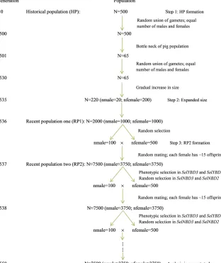
randomly selected from the RP1 as the founders of recent population 2 (RP2). The RP2 had 13 generations (generation 2537–2550). For each of these generations, 100 males and 500 females who either had the highest phenotypic values (for a scenario with phenotypic selection) or were randomly selected (for a scenario with no selection) from the former generation were kept as parents for the next generation. Each female had15 progeny (from 7 to 22) to mimic a real pig population. The sex ratio for the progeny wasfixed as 0.5. For the last generation in RP2, there were7500 individuals in total. All the simulation steps were repeated 10 times to cre-ate 10 independent data sets for the further analysis.

The genome consisted of 18 autosomes of 120 cM each. For the first generation in the HP, each chromosome had 200 segregating biallelic QTLloci and 18,200biallelic marker loci randomly located (thus, in total, 3600 QTL loci and 327,600 marker loci). In thefirst generation, allele frequencies for QTL and markers loci were 0.5, and the recurrent mutation rate was 2:531024_:

Since software QMSim cannot simulate dominance effects, in the RP2 (from generation 2537 onwards), the option of “ebv_est = external_bv”in QMSim was used to base selec-tion decisions on a user providedfile. In this study, selection

decisions were made according to phenotypic values (phenotypic selection) and thus, the provided file contained user-defined phenotypes for each individual.

These phenotypic values were simulated as follows. For each QTL, additive effectsaand dominance effectsdwere constant across generations. The additive effectsaof 3600 QTL loci were drawn from a Student’st-test distribution with 2.5 d.f. [a¼rtð3600;2:5Þ in R] (Wellmann and Bennewitz 2012). Then, dominance functional effectsdwere drawn in two differ-ent ways:BayesD2andBayesD3, as is proposed in Wellmann and Bennewitz (2012). ForBayesD2, the magnitudes ofaandd

were related asd¼djajandcorðdi;jaijÞ ¼0:Bennewitz and Meuwissen (2010) showed that dominance coefficientsd fol-low a normal distribution with mean 0.193 and SD 0.312. Therefore, the dominance coefficients were simulated as

d¼rnormð3600;mean¼0:193;sd¼0:312Þ and d¼djaj

(element-wise multiplication) in R. For the BayesD3, the magnitudes of a and d were related as d¼djaj and corðdi;jaijÞ.0: Wellmann and Bennewitz (2012) assumed dominance coefficientsdfollow a conditional normal dis-tribution as djjaj NðmDðjaj=sÞ;s2DÞ;where s is a scaling

parameter andmDðxÞ ¼x=ðsDþxÞwithsD.0. To generate

the dominance coefficients d following a distribution similar to that in BayesD2, s_D¼4 was chosen and

d¼ jaj=ð4þ jajÞ þ0:3*rnormð3600Þ was used in R for BayesD3. The bivariate plots betweenaanddin the 10 sim-ulated data sets are shown in the supplementalfiles (Supple-mental Material, Figure S1 for BayesD2 and Figure S2 for BayesD3). The mean empirical correlation (s.e.) between jajanddover 10 repetitions was,20:000013 ð0:0015Þ for BayesD2and¼0:355 ð0:039ÞforBayesD3.

Then, for each individual, based on the genotypes of 3600 QTL loci and the corresponding QTL effects,“true” geno-typic additive effectsuand dominance effectsvof each indi-vidual were calculated. Residual effects were sampled from a normal distribution. Afterward, the phenotype for each indivi-dual was calculated as the sum of an overall mean, true additive effects, dominance effects, and residual effects. Internally, QMSim used these phenotypes as the selection criteria for the next generation in scenarios with selection. In scenarios with no selection, replacement at each generation was done at random. At the last generation of RP2, on average650 QTL loci were segregating. Once the simulation wasfinished, each SNP marker simulated by QMSim was retained for the subsequent analyses if the minor allele frequency was larger than 0.05. In total, there were50K segregating markers retaining. The parameterfile for QMSim can be found in the supplemental material.

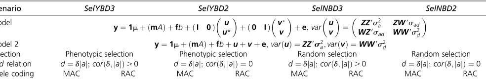
Four scenarios were studied (Table 2). Two scenarios had phenotypic selection: SelYBD3 (“Selection Yes BayesD3”), where a and d were related as in BayesD3; and SelYBD2 (“Selection Yes BayesD2”), wherea anddwere related as in BayesD2. Two scenarios had no selection: SelNBD3 (“Selection No BayesD3”) and SelNBD2 (“Selection No BayesD2”), withaanddrelated as inBayesD3andBayesD2, respectively. Within each scenario, MAC (most frequent allele as reference) in combination with M1 and M2 (M1-MAC and M2-MAC) and RAC (random allele as reference) in combina-tion with M1, M2, and M3 (M1-RAC, M2-RAC, and M3-RAC) were applied. For each scenario, 10 replicates were run.

Predictive abilities

The effect on predictive abilities of including the covariance between the genotypic additive and dominance effects in the genomic model was investigated. Prediction was performed

by using M1, M2, and M3 in the scenarios with selection. In each replicate, 20% of individuals in the last generation of RP2 were randomly masked and put into the validation population; the remaining 80% of individuals were used as the training population. The predictive ability was measured as the corre-lation, in the validation popucorre-lation, between true total genetic valuesgthat were known from the simulation and the esti-mated total genetic values^g¼mA^þf^bþ^uþ^vfor MAC and ^

g¼f^bþu^þ^vfor RAC. Bias was measured as the regression coefficient of totalgon estimated genetic values^g. The Hotelling– Williamst-test at a 95% confidence level was applied to evaluate the significance for the differences of predictive abilities between M1, M2, and M3 within different scenarios. Table 2 summarizes the analyses for the different scenarios.

Data availability

The authors state that all data necessary for confirming the conclusions presented in the manuscript are represented fully within the manuscript. Supplemental material available at Figshare:https://doi.org/10.25386/genetics.6111068.

Results and Discussion

Regressions on proportion of most frequent alleles and on genomic inbreeding in M1

Average regression coefficients (s.e.) of phenotypes on the proportion of the most frequent alleles (A) in the model were 12.61 (1.32) for SelYBD3, 12.10 (1.97) for SelYBD2, 0.02 (2.32) forSelNBD3, and 0.02 (2.51) forSelNBD2. The posi-tive Afor scenarios with selection is in agreement with the tendency that after long-term selection, additive effects for most frequent alleles are positive. The average (s.e.) inbreed-ing depression parameters per unit of inbreedinbreed-ing (b) were 26.36 (1.73) forSelYBD3,26.20 (1.45) forSelYBD2,26.63 (1.34) for SelNBD3, and 26.18 (1.52) forSelNBD2. These negative inbreeding depression parameters confirm the phe-nomenon of inbreeding depression.

Variance components

Variance components were calculated using QTL (to obtain the true values) and also, using markers, for the four scenarios combining models M1 (with correlated additive and

Table 2 Summary for different scenarios

Scenario SelYBD3 SelYBD2 SelNBD3 SelNBD2

Model

y¼1mþ ðmAÞ þfbþ ðI 0Þ

u u*

þ ð0 IÞ

v*

v

þe;var

u v

¼

ZZ9s2a ZW9sad WZ9sad WW9s2d

Model 2 y¼1mþ ðmAÞ þfbþuþvþe;varðuÞ ¼ZZ9s2

a;varðvÞ ¼WW9s2d

Selection Phenotypic selection Phenotypic selection Random selection Random selection a;drelation d¼djaj;corðd;jajÞ.0 d¼djaj;corðd;jajÞ ¼0 d¼djaj;corðd;jajÞ.0 d¼djaj;corðd;jajÞ ¼0

Allele coding MAC RAC MAC RAC MAC RAC MAC RAC

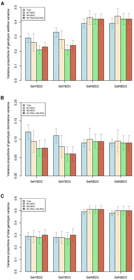
dominant genotypic effects) or M2 (with uncorrelated effects) with MAC (most frequent allele as reference) or RAC (random allele as reference). This gives four combinations (M1-MAC, M2-MAC, M1-RAC, and M2-RAC). Results were the mean of 10 replicates. Variance proportions of genotypic additive (h2

u), genotypic dominance (h2

v), and total genotypicðH2Þvariance

over phenotypic variance are presented in Figure 2. All the other variance components are in Table S1 in the supplemen-tal material.

For scenarios with phenotypic selection (SelYBD2 and SelYBD3), estimated variance components in M1-MAC were not statistically significantly different from the true ones,

while results in the other cases (M1-RAC, MAC, and M2-RAC) were slightly but statistically different from the true ones. Similarly, all the calculated genetic parameters (h2u; h2

v andH

2_{) in M1-MAC were not significantly different from}

the true values, while values in the other cases (M1-RAC, M2-MAC, and M2-RAC) were slightly different from the true ones in these two scenarios.

For scenarios with random selection (SelNBD2 and SelNBD3), estimated genetic parameters in different cases did not dramatically deviate from the true ones. In all cases,

s2u;h2u andH2 values were slightly overestimated. Estimates from M1-MAC did not show advantages over those from other combinations.

Overall, the variance components estimated with model M1 were close to the true values in different scenarios. In animal and plant breeding, most traits have experienced long-term selection. Thus, to estimate the genetic parameters more precisely, a genomic model considering covariances between genotypic ad-ditive and dominance effects (like M1) seems appropriate.

Genetic correlations

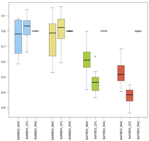
True and estimated genetic correlations between genotypic additive effects and genotypic dominance effects (ru;v) for combinations M1-MAC and M1-RAC in different scenarios are shown in Figure 3. When RAC was used, the ru;v was almost 0 in any scenario. However, when the most frequent allele was the reference (MAC), scenarios with phenotypic selection (SelYBD3andSelYBD2) yielded negative estimates

ofru;v:In such two scenarios, the absolute values of estimated ru;v were slightly lower than the absolute values of trueru;v: For scenarios with random selection (SelNBD3andSelNBD2), both true and estimatedru;vwere around zero.

Results showed that whenaanddare related (Bennewitz and Meuwissen 2010; Wellmann and Bennewitz 2012), a negative correlation may be generated between the geno-typic additive and dominance effects after long-term selec-tion. The long-term directional selection seems to be a precondition for producing such correlation. M1-MAC can cap-ture part of such correlation.

LRT

The goodness of fit of M1 and M2 in different scenarios is shown as22logðlikelihoodÞin the third and fourth columns in Table 3 for both MAC and RAC, respectively. For each allele coding way, M1 always had smaller numeric values of 22logðlikelihoodÞthan M2 within different scenarios, which indicated that the M1fitted the data set better than the M2. For all the four scenarios, LRT showed no significant dif-ferences infitting the data set between M1 and M2 (p.0:05) when RAC was applied. However, when MAC was used, M1 fitted the data set significantly better than M2 in scenarios with phenotypic selection (SelYBD3andSelYBD2). For sce-narios with random selection (SelNBD3andSelNBD2), there were no significant differences of goodness offit between M1 and M2, no matter which allele coding was applied. However, it can be seen that within each scenario, there was a tendency that M1fitted the data set better than M2, which suggested that a genomic model including the relationships between genotypic additive and dominance effects fits the simu-lated data better than a model without considering such relationships.

Predictive abilities

Based on the results of LRT, M1 only provided a betterfit for the data set than M2 in scenarios with phenotypic selection (SelYBD3andSelYBD2) when MAC was used for coding SNP markers. Besides, in animal breeding, most traits have expe-rienced long-term selection. Therefore, predictive abilities

Figure 3 Genetic correlations between genotypic additive and domi-nance effects based on model 1 in different scenarios across 10 repeti-tions. QTL indicate the true correlations that were calculated based on QTL; either MAC and RAC was applied to code genotypes.SelNBD2,SelNBD3, SelYBD2, andSelYBD3were the four studied scenarios. MAC, major allele coding; RAC, random allele coding;SelNB, Selection No Bayes;SelYB, Se-lection Yes Bayes.

Table 3 Average goodness offit and22logðlikelihoodÞof M 1 and M2 across 10 repetitions, and likelihood ratio test between M1 and M2 in different scenarios

Scenario MatrixZcoding M1 M2 x2_{value P-value}

SelYBD3 MAC 25463.49 25437.12 26.37 1.41e27 RAC 25385.44 25384.91 0.88 0.1741 SelYBD2 MAC 25412.52 25398.66 13.90 9.64e25

RAC 25305.91 25303.72 2.19 0.0695 SelNBD3 MAC 24643.10 24640.99 2.10 0.0736 RAC 24637.95 24636.43 1.52 0.1095 SelNBD2 MAC 24524.30 24523.15 1.16 0.1407 RAC 24520.11 24518.41 1.70 0.0961

MAC and RAC represent allele coding applied to code genotypes; SelNBD2,

obtained from using M1 and M2 were only compared in these two scenarios (M1-MAC and M2-MAC). Predictive abilities were also computed for M2-RAC, because this model is com-monly used in other dominance studies (Su et al. 2012; Vitezica et al. 2016; Xiang et al. 2016). Furthermore, M3-RAC was also applied so that the predictive abilities from coding genotypes in a classical (orthogonal) manner (Falconer and Mackay 1996; Vitezica et al. 2013) can be compared to that from coding genotypes in a genotypic man-ner directly.

Predictive abilities and unbiasedness in different scenarios are compared in Table 4. Overall, the Hotelling–Williams t-test indicated that predictive abilities from M1 were signif-icantly higher than those from M2 (p,0:05), but similar to those from M3 (p.0:05). When MAC was applied, predic-tive abilities from M1 (M1-MAC) were1% and 0.4% higher than those from M2 (M2-MAC) for SelYBD3 and SelYBD2, respectively. This result is in agreement with LRT showing that goodness offit of M1 was significantly superior to that of M2. In addition, it also implies that the relationships between additive and dominant effects were appropriately captured. The differences of predictive abilities between M1-MAC and M2-RAC increased to 1.6% and 0.7% for SelYBD3 and SelYBD2, respectively. These differences indi-cated that consideration of the covariance between genotypic additive and dominance effects via using MAC would possi-bly generate a small extra genetic gain. For M2, when MAC was applied (M2-MAC), the predictive abilities were0.7% and 0.3% higher than using RAC (M2-RAC). This result in-dicated that predictive abilities benefited from the inclusion of regression of phenotype on the proportion of the most frequent alleles in the model, even if the covariance between additive and dominance effects were not considered in the M2. This result again recommends the use of MAC in other genomic evaluation models to enhance their predictive abil-ities, which is in line with the smaller numeric values of 22logðlikelihoodÞfor M1 than for M2. In terms of unbiased-ness, the regression coefficients observed from M1 were slightly closer to 1 than those from M2 in scenarioSelYBD2, but there was no clear trend in scenarioSelYBD3.

However, when comparing the predictive abilities from RAC with other combinations, except for M1-MAC, M3-RAC performed slightly better than M2-MAC and M2-M3-RAC. This phenomenon indicates that when the covariance

between additive and dominant effects is ignored, genomic evaluation via coding genotypes in the genotypic manner may work worse than coding genotypes in the classical, orthogonal manner (in terms of breeding values and dominance devia-tions). However, when considering the covariance between additive and dominance effects, coding genotypes in the MAC (M1-MAC) increased predictive abilities0.7% and 0.3% compared to M3-RAC, which suggested the use of MAC in combination with models considering the covariance be-tween additive and dominant effects. In terms of unbiased-ness, the regression coefficients observed from M3 were slightly further from 1 than those from M1 and M2.

Overall, the comparisons of the different models and allele codings confirmed that the predictive ability of a genomic model could slightly improve if the su;v is included (M1-MAC). The inclusion of such covariance does not need extra computing time. The computing time for estimating variance components is similar for M1-MAC and M2-MAC, which is slightly shorter than that for M3-RAC/M3-MAC.

Wellmann and Bennewitz (2012) also derived an reproduc-ing kernel Hilbert space (RKHS) model for estimatreproduc-ing total genetic values that assumed a correlation between additive and dominance effects, which was also a genomic BLUP model. This model was derived on the basis of BayesD2. A property in the RKHS model is that the covariance among two genotypic values depends on the assumeda priorijoint distribution ofaandd,i.e.,varðaÞ;varðdÞ, andcovða;dÞ;which were obtained from theoretical arguments and used for com-puting the Kernel matrix. We prefer instead to estimate these parameters explicitly from the data sets. Even though standard software can be used for prediction in the RKHS model, it cannot be used for the estimation of genetic parameters.

Conclusions

Wefirst presented a novel and simple way of incorporating, in populations under selection, the correlation between geno-typic additive and dominance effects in a genomic model that can be implemented using standard mixed model software. Our study showed that: if the population is in HW equilibrium and the absolute additive effects and dominance coefficients of QTL are positively correlated [e.g.,BayesD3in Wellmann and Bennewitz (2012)], after directional selection, a nega-tive correlation between genotypic addinega-tive and dominance effects is expected. A genomic model based on a reference

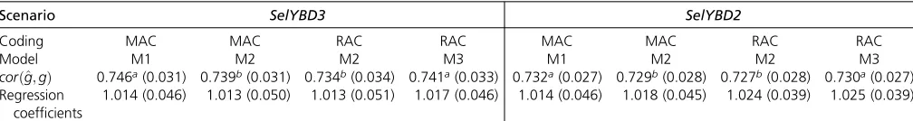
Table 4 Average predictive abilities and regression coefficients of total genetic values on predicted total genetic values with the respective SE in scenariosSelYBD3andSelYBD2

Scenario SelYBD3 SelYBD2

Coding MAC MAC RAC RAC MAC MAC RAC RAC

Model M1 M2 M2 M3 M1 M2 M2 M3

corðg^;gÞ 0.746a_{(0.031) 0.739}b_{(0.031) 0.734}b_{(0.034) 0.741}a_{(0.033) 0.732}a_{(0.027) 0.729}b_{(0.028) 0.727}b_{(0.028) 0.730}a_(0.027)

Regression coefficients

1.014 (0.046) 1.013 (0.050) 1.013 (0.051) 1.017 (0.046) 1.014 (0.046) 1.018 (0.045) 1.024 (0.039) 1.025 (0.039)

SelYBD2andSelYBD3were the two scenarios with phenotypic selection; M1, M2, and M3 indicate models 1, 2, and 3, respectively. Numbers in the parenthesis are the SE. MAC, major allele coding; RAC, random allele coding;SelYB, Selection Yes Bayes.

allele that is the most frequent one at each locus can capture part of the negative genetic correlation between genotypic additive and dominant effects, but this cannot be captured if the RAC is used. This new approach is applied to a directional selected trait controlled by both additive and dominant gene actions. When such correlation is taken into account in the model, accuracies of estimated total genetic values can be improved by up to 1.5% in genomic evaluation while bias is slightly reduced.

Acknowledgments

T.X. was supported by the Fundamental Research Funds for the Central Universities (project number 2662018QD001). O.F.C. was supported by the center for Genomic Selection in Animals and Plants (GenSAP) funded by the Danish Council for Strategic Research. A.L. and Z.G.V. thank financing from INRA SelGen metaprogram projects X-Gen and SelDir. We are grateful to the genotoul bioinformatics platform Toulouse Midi-Pyrenees (Bio-info Genotoul) for providing computing resources. Useful comments from two anonymous reviewers are acknowl-edged.

Literature Cited

Aliloo, H., J. E. Pryce, O. González-Recio, B. G. Cocks, and B. J. Hayes,

2016 Accounting for dominance to improve genomic evaluations

of dairy cows for fertility and milk production traits. Genet. Sel.

Evol. 48: 8.https://doi.org/10.1186/s12711-016-0186-0

Aliloo, H., J. Pryce, O. González-Recio, B. Cocks, M. Goddardet al.,

2017 Including nonadditive genetic effects in mating

pro-grams to maximize dairy farm profitability. J. Dairy Sci. 100:

1203–1222.https://doi.org/10.3168/jds.2016-11261

Bennewitz, J., and T. Meuwissen, 2010 The distribution of QTL

additive and dominance effects in porcine F2 crosses. J. Anim.

Breed. Genet. 127: 171–179.

https://doi.org/10.1111/j.1439-0388.2009.00847.x

Bennewitz, J., C. Edel, R. Fries, T. H. Meuwissen, and R. Wellmann,

2017 Application of a Bayesian dominance model improves power

in quantitative trait genome-wide association analysis. Genet. Sel.

Evol. 49: 7.https://doi.org/10.1186/s12711-017-0284-7

Caballero, A., and P. D. Keightley, 1994 A pleiotropic nonadditive

model of variation in quantitative traits. Genetics 138: 883_–900.

Charlesworth, B., and D. Charlesworth, 2010 Elements of

Evolu-tionary Genetics. Roberts and Company Publishers, Greenwood Village, CO.

Crow, J. F., and M. Kimura, 2009 An Introduction to Population

Genetics Theory. Blackburn Press, Caldwell, NJ.

Ertl, J., A. Legarra, Z. G. Vitezica, L. Varona, C. Edel et al.,

2014 Genomic analysis of dominance effects on milk

produc-tion and conformaproduc-tion traits in Fleckvieh cattle. Genet. Sel. Evol.

46: 40.https://doi.org/10.1186/1297-9686-46-40

Falconer, D. S., and T. F. C. Mackay, 1996 Introduction to

Quan-titative Genetics, Ed. 4. Pearson Education Limited, LONGMAN, Harlow, United Kingdom.

Fernández, E., A. Legarra, R. Martínez, J. P. Sánchez, and M.

Base-lga, 2017 Pedigree-based estimation of covariance between

dominance deviations and additive genetic effects in closed rab-bit lines considering inbreeding and using a computationally

simpler equivalent model. J. Anim. Breed. Genet. 134: 184_–

195.https://doi.org/10.1111/jbg.12267

Gilmour, A. R., B. Gogel, B. Cullis, R. Thompson, and D. Butler, 2009 ASReml User Guide Release 3.0. VSN International Ltd, Hemel Hempstead, United Kingdom.

Hill, W. G., M. E. Goddard, and P. M. Visscher, 2008 Data and theory

point to mainly additive genetic variance for complex traits. PLoS

Genet. 4: e1000008.https://doi.org/10.1371/journal.pgen.1000008

Legarra, A., 2016 Comparing estimates of genetic variance across

different relationship models. Theor. Popul. Biol. 107: 26–30.

https://doi.org/10.1016/j.tpb.2015.08.005

Lynch, M., and B. Walsh, 1998 Genetics and Analysis of

Quantita-tive Traits. Sinauer Associates Inc, Sunderland, MA.

Madsen, P., and J. Jensen, 2013 A User’s Guide to DMU. Version 6,

Release 5.2. Center for Quantitative Genetics and Genomics. Dept. of Molecular Biology and Genetics. Aarhus University, Tjele, Denmark.

Misztal, I., S. Tsuruta, T. Strabel, B. Auvray, T. Druet et al.,

2002 BLUPF90 and related programs (BGF90). Proceedings

of the 7th World Congress on Genetics Applied to Livestock

Production. Montpellier, France, pp. 21–22.

Muñoz, P. R., M. F. Resende, S. A. Gezan, M. D. V. Resende, G. de

los Camposet al., 2014 Unraveling additive from nonadditive

effects using genomic relationship matrices. Genetics 198:

1759–1768.https://doi.org/10.1534/genetics.114.171322

Sargolzaei, M., and F. S. Schenkel, 2009 QMSim: a large-scale

genome simulator for livestock. Bioinformatics 25: 680–681.

https://doi.org/10.1093/bioinformatics/btp045

Silió, L., C. Barragán, A. I. Fernández, J. García-Casco, and M. C.

Rodríguez, 2016 Assessing effective population size,

coances-try and inbreeding effects on litter size using the pedigree and SNP data in closed lines of the Iberian pig breed. J. Anim. Breed.

Genet. 133: 145–154.https://doi.org/10.1111/jbg.12168

Sorensen, D., R. Fernando, and D. Gianola, 2001 Inferring the

trajectory of genetic variance in the course of artificial selection.

Genet. Res. 77: 83–94 (erratum: Genet. Res. 77: 297).

Speed, D., and D. J. Balding, 2015 Relatedness in the post-genomic

era: is it still useful? Nat. Rev. Genet. 16: 33_–44.https://doi.org/

10.1038/nrg3821

Su, G., O. F. Christensen, T. Ostersen, M. Henryon, and M. S. Lund,

2012 Estimating additive and non-additive genetic variances

and predicting genetic merits using genome-wide dense single nucleotide polymorphism markers. PLoS One 7: e45293.

https://doi.org/10.1371/journal.pone.0045293

Vitezica, Z. G., L. Varona, and A. Legarra, 2013 On the additive

and dominant variance and covariance of individuals within the

genomic selection scope. Genet. 194: 1223–1230. https://doi.

org/10.1534/genetics.113.155176

Vitezica, Z. G., L. Varona, M. J. Elsen, I. Misztal, W. Herring et al.,

2016 Genomic BLUP including additive and dominant variation

in purebreds and F1 crossbreds, with an application in pigs. Genet.

Sel. Evol. 48: 6.https://doi.org/10.1186/s12711-016-0185-1

Wang, L., P. Sørensen, L. Janss, T. Ostersen, and D. Edwards,

2013 Genome-wide and local pattern of linkage

disequilib-rium and persistence of phase for 3 Danish pig breeds. BMC

Genet. 14: 115.https://doi.org/10.1186/1471-2156-14-115

Wellmann, R., and J. Bennewitz, 2011 The contribution of

domi-nance to the understanding of quantitative genetic variation. Genet.

Res. 93: 139–154.https://doi.org/10.1017/S0016672310000649

Wellmann, R., and J. Bennewitz, 2012 Bayesian models with

dom-inance effects for genomic evaluation of quantitative traits. Genet.

Res. 94: 21–37.https://doi.org/10.1017/S0016672312000018

Xiang, T., O. F. Christensen, Z. G. Vitezica, and A. Legarra,

2016 Genomic evaluation by including dominance effects

and inbreeding depression for purebred and crossbred perfor-mance with an application in pigs. Genet. Sel. Evol. 48: 98.

Appendix A

Here, we consider di¼dijaij and argue that it often holds that covðai;diÞ.0 when covðdi;jaijÞ.0 [BayesD3 model in Wellmann and Bennewitz (2012)] and covðai;diÞ ¼0 whencovðdi;jaijÞ ¼0 [BayesD2model in Wellmann and Bennewitz (2012)].

In the main part of the paper, we have derived that the covariance between additive and dominance effects is determined by VarðdiÞ; and since Eðd2

iÞ ¼Eðd

2

ia2iÞ ¼Eðd

2

iÞEða2iÞ þcovðd

2

i;a2iÞ;and EðdiÞ ¼EðdijaijÞ ¼EðjaijÞEðdiÞ þcovðdi;jaijÞ; we see that the result holds whencovðd2i;a2iÞ2covðdi;jaijÞ222EðjaijÞEðdiÞcovðdi;jaijÞ.0 whencovðdi;jaijÞ.0;andcovðd2i;a2iÞ ¼0 when covðdi;jaijÞ ¼0: This latter property often holds; for example it holds when covðd2i;a

2

iÞ ¼2covðdi;jaijÞ2þ 4EðjaijÞEðdiÞcovðdi;jaijÞ;which we show below to hold for the bivariate normal case.

Here, we derive an expression forcovða2_;

d2Þwhen assuming a bivariate normal distribution onðd;jajÞ:For simplicity of notation assume thatm1¼EðjajÞ; m2¼EðdÞ;s21¼varðjajÞ; s22¼varðdÞands12¼covðd;jajÞ;and define the centered

ran-dom variables X1¼ jaj2m1 and X2¼d2m2: First, we write covða2;d2Þ ¼covðX12;X22Þ þ2m1covðX1;X22Þ þ2m2covðX12;X2Þ;

which reduces tocovða2_;

d2Þ ¼EðX2

1;X22Þ2s21s22þ2m1EðX1X22Þ þ2m2EðX12X2Þ þ4m1m2EðX1X2Þ:For the bivariate normal

dis-tribution the central moments are EðX2

1X22Þ ¼s21s22þ2s212; EðX1X22Þ ¼EðX12X2Þ ¼0 and EðX1X2Þ ¼s12;and from this we

obtain thatcovða2_;

d2Þ ¼2s212þ4m1m2s12:

Finally, we note that, strictly speaking, jaj cannot follow a normal distribution, so the above expression is only an approximation.

Appendix B

Consider a set of individuals with genetic values (in a broad sense, these can be understood as genotypic values)g;and these genetic values are assumed drawn from a certain distribution,i.e.,EðgÞ ¼0andVarðgÞ ¼Gs2g:Since the genetic values are unknown and drawn from a sampling distribution, the variances of these genetic values will also have a certain distribution (Sorensen et al.2001; Legarra 2016). Legarra (2016) showed that, on average, the expectation of the variance for these genetic values is VG¼ ðdiagðGÞ2GÞs2g¼Dgs2g;wherediagðGÞis the average of the diagonal ofGandG is the average of matrixG;andDgis the difference between the two. Thus, the expected varianceVGis associated with relationship matrixG: Only ifDgis equal to 1, the expectation of variance for genetic valuesVGcan be identical to the estimated variance component

s2

g(Speed and Balding 2015). In this study, the submatricesZZ9=k;ZW9=k;andWW=9kdo not yield respectiveDZZ9=k;DZW9=k;and DWW9=k equal to 1. Thus, the estimated variance components were scaled to the expected variance components of a population using, for instance,DZW9=k¼diagðZW9=kÞ2ðZW9=kÞandCovuv¼DZW9=ks*ad:

The values of the statistics can be derived analytically. For one SNP locus, if the population is in Hardy–Weinberg equilibrium andpis the frequency of the allele whose homozygote has the genotypic valuea;the frequencies of different genotypes in theZ

andWmatrices for one locus are:

p2 _{2pq q}2 Z 1 0 21

W 0 1 0

Therefore, the elements in the matrixZW9=kwith corresponding frequencies are: p2 _{2pq q}2

p2 _{0 1=k 0}

2pq 0 0 0

q2 0 21=k 0

For instance, in a one-locus model, value 1=kappears with frequency 2pq(the number of animals heterozygote) timesp2_(the

number of homozygotes) in matrixZW9=k:Extending the reasoning to all loci, from the above table,diagðZW9=kÞ ¼0 (because an individual cannot be homozygote and heterozygote at the same time);ðZW9=kÞ ¼1

k

P_​

2piqiðp2i 2q2iÞ ¼1k

P_​

2piqið2pi21Þ;where k¼ ftrðKÞg=2n¼ ðp4_þq4_þ4p2_q2_{Þ=2.0: Thus, D}

ZW9=k¼diagðZW9=kÞ2ðZW9=kÞ ¼ 21k

P_​

2piqið2pi21Þ: If p.0:5 (MAC), DZW9=kis negative because

P_​ð

2pi21Þ.0;but if RAC is used thenDZW9=k¼0 because

P_ð​