University of Windsor University of Windsor
Scholarship at UWindsor
Scholarship at UWindsor
Electronic Theses and Dissertations Theses, Dissertations, and Major Papers
2009
Shallow wake in open channel flow - a look into the vertical
Shallow wake in open channel flow - a look into the vertical
variability
variability
Arindam Singha University of Windsor
Follow this and additional works at: https://scholar.uwindsor.ca/etd
Recommended Citation Recommended Citation
Singha, Arindam, "Shallow wake in open channel flow - a look into the vertical variability" (2009). Electronic Theses and Dissertations. 466.
https://scholar.uwindsor.ca/etd/466
SHALLOW WAKE IN OPEN CHANNEL FLOW
- A LOOK INTO THE VERTICAL VARIABILITY
by
Arindam Singha
A Dissertation
Submitted to the Faculty of Graduate Studies
through Mechanical, Automotive and Materials Engineering
in Partial Fulfillment of the Requirements for
the Degree of Doctor of Philosophy at the
University of Windsor
Windsor, Ontario, Canada
2009
Shallow wake in Open Channel Flow – A look into the Vertical
Variability
by
Arindam Singha
APPROVED BY:
_____________________________ V. Chu, External Examiner
McGill University
_____________________________ S. Cheng
Department of Civil & Environmental Engineering
____________________________ R. Barron
Department of Mechanical, Automotive & Materials Engineering and Department of Mathematics & Statistics
_____________________________ G. Rankin
Department of Mechanical, Automotive & Materials Engineering
________________________ R. Balachandar, Advisor
Department of Mechanical, Automotive & Materials Engineering
__________________________ T. Bolisetti, Chair of Defense
Department of Civil & Environmental Engineering
Declaration of Co-Authorship / Previous Publication
I. Co-Authorship Declaration
I hereby declare that this thesis incorporates material that is result of joint research, as follows:
This thesis incorporates outcome of a research undertaken under the supervision of Dr. Ram Balachandar. The collaboration is covered in chapter 2, 4, 5 and 6 of the thesis. In all cases, the key ideas, primary contributions, experimental designs, data analysis and interpretation, were performed by the author, and the contributions of the co-authors was primarily through the provision of supervision.
I am aware of the University of Windsor Senate Policy on Authorship and I certify that I have properly acknowledged the contribution of other researchers to my thesis, and have obtained written permission from each of the co-author(s) to include the above material(s) in my thesis.
I certify that, with the above qualification, this thesis, and the research to which it refers, is the product of my own work.
II. Declaration of Previous Publication
This thesis includes 3 original papers that have been previously published/submitted for publication in peer reviewed journals, as follows:
Thesis Chapter Publication title/full citation Publication status Chapter 4 PIV-POD investigation of the wake of of a
sharp-edged bluff body immersed in shallow channel flow, J. Fluids Engg.
Published
Chapter 5 Vertical variability of the wake of a sharp-edged bluff body immersed in a shallow
channel flow, Phy. Fluids
Chapter 5 Coherent structure statistics in the wake of a sharp-edged bluff body placed vertically in a shallow channel flow, Phys. Fluids
Submitted
I certify that I have obtained a written permission from the copyright owner(s) to include the above published material(s) in my thesis. I certify that the above material describes work completed during my registration as graduate student at the University of Windsor.
I declare that, to the best of my knowledge, my thesis does not infringe upon anyone’s copyright nor violate any proprietary rights and that any ideas, techniques, quotations, or any other material from the work of other people included in my thesis, published or otherwise, are fully acknowledged in accordance with the standard referencing practices. Furthermore, to the extent that I have included copyrighted material that surpasses the bounds of fair dealing within the meaning of the Canada Copyright Act, I certify that I have obtained a written permission from the copyright owner(s) to include such material(s) in my thesis.
Abstract
The vertical variability of a typical wake behind a bluff body in an open channel flow has
been investigated. The focus of the study was to explore the variability of the flow
structures in terms of mean velocity profiles, turbulent parameters and coherent
structures. A sharp-edged bluff body was chosen to minimize the effect of Reynolds
number and ensure fixed flow separation points in the vertical direction. Velocity
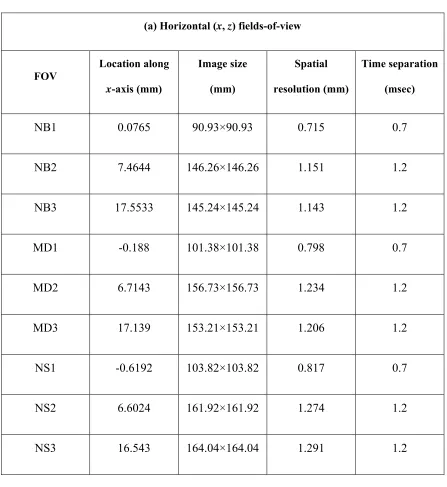
measurement was performed using particle image velocimetry at three vertical locations:
near-bed, mid-depth and near the free surface. In the streamwise direction, three different
fields-of-view were considered to cover a distance 10 times the width of the body. At all
locations, 2000 image pairs of 2048×2048 pixel resolution were acquired at a sampling
frequency of 1 Hz. Proper orthogonal decomposition (POD) was used as a tool to educe
information about the coherent structures in the flow. A robust closed-streamline based
coherent structure identification algorithm was developed to systematically detect the
presence of the coherent structures in the flow. This step was followed by a statistical
study of the location, size and strength of the coherent structures.
The results show that the bed and the free surface, as well as the approaching vertically
sheared flow have a significant effect on the structure of the wake. The bed was found to
restrict the transverse growth of the wake, whereas the free surface enhances the turbulent
energy redistribution at the free surface. The size, shape and the development of the
recirculation zone behind the bluff body also indicates vertical variability. Analysis based
on signed swirling strength indicates rapid dissipation of vorticity at the near-bed region,
structures was found to be largest at the mid-depth location, and smallest at the near-bed
location. Also, the strength of the structures was found to be smaller at the near-bed
location, compared to other vertical locations. Indirect evidence of the merging of the
Dedication
To
My Motherland, India,
and
Acknowledgements
I am indebted to my supervisor, Dr. Ram Balachandar, for his distinguishing supervision
and support. In addition to encouraging independence in work and providing excellent
facilities, Dr. Balachandar’s thought provoking quaries and suggestions have been
instrumental for the timely completion of the present work.
I sincerely acknowledge my gratitude to my committee members Dr. R. Barron, Dr. G.
Rankin and Dr. S. Cheng for their valuable time and suggestions for the study. A special
thanks to Dr. Barron for meticulously proof reading the document.
Next only in importance in the contribution to the current dissertation is Dr. A Shinneeb,
who has been kind enough to teach me the fundamentals of experimentation and
programming. Additional thanks to Vesselina for her help and the endless discussions we
have to come up with new ideas. Last but not the least, thanks go to my friends at the
University of Windsor; Arjun, Anirban, Faruqubhai, Barsha, Ben, Tian, Anupam, Sanjib,
Sarmistha, Miltonbhai. Special thanks to Matt St. Louis, for letting me borrow everything
from his workshop in aid of my expriments. Heart-felt acknowledgement goes to Tim
Table of Contents
Declaration of Co-Authorship / Previous Publication ... iii
Abstract ... v
Dedication ... vii
Acknowledgements ... viii
List of Figures ... xiv
List of Tables ... xxi
Nomenclature ... xxii
Chapter 1 INTRODUCTION ... 1
1.1 Shallow flows ... 1
1.2 Practical occurrences of shallow wake ... 2
1.3 Motivation ... 4
1.4 Scope ... 6
Chapter 2 LITERATURE REVIEW ... 11
2.1 General remarks ... 11
2.2 Introduction ... 11
2.3 Shallow channel flow ... 12
2.3.1 Near-bed region ... 13
2.3.2 Near free surface region ... 16
2.4 Shallow wake ... 20
2.4.1 Stability number ... 22
2.4.2 Effect of the bed... 25
2.4.3 Effect of the free surface ... 28
2.4.4 Effect of the approaching velocity ... 30
2.4.5 Two-dimensional coherent structures ... 32
2.4.6 Related literatures and vertical variability of shallow wake ... 35
Chapter 3 EXPERIMENTAL DETAILS ... 53
3.1 General comments ... 53
3.2 Experimental setup ... 53
3.2.1 Open channel recirculating flume ... 53
3.2.2 Bluff body ... 54
3.2.3 Measurement locations and details ... 54
3.3 Particle image velocimetry ... 55
3.3.1 Flow seeding with tracer particles ... 57
3.3.2 Illumination of the flow field ... 58
3.3.3 Image recording ... 59
3.3.4 Image processing ... 60
3.3.5 Removal and replacement of spurious vectors ... 62
3.4 Proper orthogonal decomposition (POD) ... 66
3.5 Coherent structure identification algorithm ... 68
Chapter 4 MEAN FLOW VARIABLES ... 82
4.1 General description ... 82
4.2 Approaching flow ... 82
4.3 Mean velocity field of the wake flow ... 84
4.3.1 Instantaneous streamline pattern ... 84
4.3.2 Velocity deficit parameter ... 85
4.3.3 Mean streamwise velocity profiles ... 86
4.3.4 Mean transverse velocity profiles ... 87
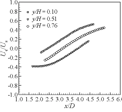
4.3.5 Variation of the streamwise velocity in the central-plane of the wake .. 89
4.3.6 Half Width of the Wake ... 89
4.3.7 Turbulent parameters ... 90
4.4 Coherent structures ... 95
4.5 Conclusions ... 100
5.1 General description ... 130
5.2 Approaching flow ... 130
5.3 Time-mean description of the flow ... 131
5.3.1 Streamwise velocity defect ... 131
5.3.2 Time averaged velocity field ... 132
5.3.3 Instantaneous streamline pattern ... 133
5.3.4 Centreline velocity deficit ... 135
5.3.5 Wake half-width ... 135
5.3.6 Entrainment coefficient ... 136
5.3.7 Turbulent fluctuations ... 137
5.3.8 Evolution of flow pattern downstream of the bluff body ... 141
5.3.9 Swirling strength analysis ... 143
5.4 Conclusions ... 148
Chapter 6 STATISTICS OF COHERENT STRUCTURES ... 183
6.1 General remarks ... 183
6.2 Eduction of large-scale structures by POD ... 183
6.3 Statistics of coherent structures ... 187
6.4 Conclusions ... 194
Chapter 7 CONCLUSIONS AND FUTURE RECOMMENDATIONS ... 216
7.1 Conclusions ... 216
7.2 Recommendations for future work ... 221
References ... 223
Appendix A Uncertainty Estimates of Velocity Measurement ... 234
7.3 Uncertainty estimates of measurement ... 234
7.3.1 Error in calibration, α ... 235
7.3.1.1 Image distance of the reference point ... 236
7.3.1.2 Physical distance from the reference point ... 236
7.3.1.4 Distortion in the CCD device ... 236
7.3.1.5 Ruler position ... 237
7.3.1.6 Ruler parallelism ... 237
7.3.2 Error in displacement of the particle image, Δx ... 237
7.3.2.1 Laser power fluctuation ... 237
7.3.2.2 Optical distortion by CCD ... 237
7.3.2.3 Normal viewing angle ... 238
7.3.2.4 Mismatching error ... 238
7.3.2.5 Sub-pixel analysis ... 238
7.3.3 Error in the time interval, Δt ... 238
7.3.3.1 Delay generator ... 239
7.3.3.2 Pulse timing accuracy ... 239
7.3.4 Error in δu ... 239
7.3.4.1 Particle trajectory ... 239
7.3.4.2 Three-dimensional effect... 239
7.3.5 Error in the measurement location, x ... 240
7.3.5.1 Centre position of the correlation area ... 240
7.3.5.2 Nonuniformity of tracer particle density ... 240
7.3.6 Error in the measurement time, t ... 240
7.4 Summary of uncertainty calculation ... 240
Appendix B MATLAB® codes ... 246
7.5 General comments ... 246
7.6 Variable outlier rejection code ... 246
7.7 Code for ensemble averaging of PIV dataset ... 259
7.8 Proper orthogonal decomposition ... 262
7.8.1 POD decomposition ... 262
7.8.2 POD reconstruction ... 265
7.9.1 Main code ... 267
7.9.2 Approximation of circle in rectangular grid(Bresenham’s algotithm) . 273 7.9.3 Detection of a clockwise structure ... 275
7.9.4 Detection of counterclockwise structure ... 277
7.10 Calculation of swirling strength from PIV dataset ... 278
Appendix C Copyright permissions ... 281
7.11 Figure 2.5 ... 281
7.12 Figure 2.6 ... 283
7.13 Figure 2.4 ... 285
7.14 Figure 2.9 ... 287
List of Figures
Figure 1.1: Vortex street of the Juan Fernandez Islands ... 8 Figure 1.2: Shallow wake behind Argo Merchant (Van Dyke, 1982). ... 9 Figure 1.3: Shallow wake in Naruto Strait and the ship stranded in the whirlpool 10 Figure 2.1: Velocity field of open channel flow at H = 0.10 m, a) mean velocity field from 2000 images, b) instantaneous velocity field, and c) corresponding fluctuating velocity field. The flow direction is from left to right. ... 41 Figure 2.2: Galilean decomposed velocity fields in (x, y) plane at Red = 2100 at (a)
UC = 0.9U0and (b) UC = 0.8U0 . ... 44
Figure 2.3: Examples of POD reconstructed velocity fields (a) using the first twelve POD modes and (b) from POD modes 13 to 100. Note that only every second vector is shown to avoid cluttering. ... 46 Figure 2.4: Qualitative demonstration of the effect of the bed on the development of shallow wake (Reproduced with the permission of American Geophysical Union). ... 47 Figure 2.5: Widening of the wake close to the free-surface (Adopted from Logory et al. 1996). The contour levels represents mean velocity, white to dark shade represents higher to lower range of streamwise velocity. θ0(= 3.1 mm) is the
half-momentum thickness of the wake (Reproduced with the permission of American Institute of Physics). ... 48 Figure 2.6: Signature of the surface currents as seen in a streamwise plane
Figure 2.8: Examples of the instability mechanisms of shallow flows ... 51
Figure 2.9: Example of deep-shallow and shallow-shallow wake (Reproduced by permission from M. Tachie) ... 52
Figure 3.1: A picture of the bluff body used in the experiment. ... 75
Figure 3.2: The open-channel flume in operation. ... 76
Figure 3.3: Schematic of the operating principle of a typical PIV system... 77
Figure 3.4: Schematic of the experimental setup (not to scale). The height of the body is 110 mm, and protrudes above the free surface. ... 78
Figure 3.5: Schematics of the process of generation of the light sheet. ... 79
Figure 3.6: An example of the image after cross-correlation analysis. ... 80
Figure 3.7: A sample field-of-view with spurious vectors. The spurious vectors are labelled as A-E. ... 81
Figure 4.1: Mean streamwise velocity distribution of the smooth channel flow using inner coordinates. ... 103
Figure 4.2: Streamline patterns of the mean velocity fields in the wake of the bluff body for three horizontal planes (a) y/H = 0.10, (b) y/H = 0.51, and (c) y/H = 0.76. ... 104
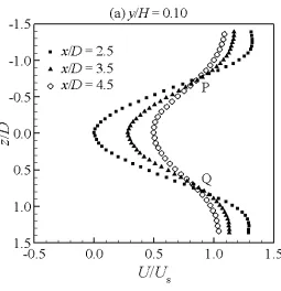
Figure 4.3: Development of the mean streamwise velocity U/Us in the streamwise direction at different horizontal planes (a) y/H = 0.10, (b) y/H = 0.51, (c) y/H = 0.76. ... 106
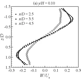
Figure 4.4: Development of the mean transverse velocity W/Us in the streamwise direction at different horizontal planes (a) y/H = 0.10, (b) y/H = 0.51, and (c) y/H = 0.76. ... 108
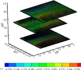
Figure 4.5: A vector plot representing the mean flow field in the three horizontal planes (y/H = 0.10, 0.51, and 0.76) superimposed by a color contour of the normalized mean transverse velocity W/Us. ... 110
Figure 4.7: Variation of the wake half-width z0.5/D with downstream distance. . 112 Figure 4.8: Development of the relative streamwise root-mean-square velocity
Urms/Us in the normalized streamwise direction for horizontal planes at (a) y/H =
0.10, (b) y/H = 0.51, and (c) y/H = 0.76. ... 113 Figure 4.9: Development of root-mean-square transverse velocity Wrms/Us in the
streamwise direction for horizontal planes at (a) y/H = 0.10, (b) y/H = 0.51, (c) y/H
= 0.76. ... 115 Figure 4.10: Development of turbulent kinetic energy in the streamwise
direction for horizontal planes at (a) y/H = 0.10, (b) y/H = 0.51, (c) y/H = 0.76. 117
2
/
U
sK
Figure 4.11: Variation of Urms/Wrms in the streamwise direction. The three curves
were extracted from the three horizontal planes along the vertical central plane (z/D = 0). ... 119 Figure 4.12: Development of Reynolds stress (<uw>/Us2) in the streamwise
direction for horizontal planes at; (a) y/H = 0.10, (b) y/H = 0.51, (c) y/H = 0.76. ... 120 Figure 4.13: Three examples showing coherent structures identified on the mid-vertical plane by the POD technique. ... 122 Figure 4.14: Examples of POD-reconstructed instantaneous velocity fields in the horizontal plane at y/H = 0.10. ... 124 Figure 4.15: Examples of POD-reconstructed instantaneous velocity fields in the horizontal plane at y/H = 0.51. ... 126 Figure 4.16: Examples of POD-reconstructed instantaneous velocity fields in the horizontal plane at y/H = 0.76. ... 128 Figure 5.1: Mean streamwise velocity distribution of the approaching flow in the inner (inset) and outer coordinates. The solid lines in the inset correspond to the theoretical velocity profile at the viscous sublayer and logarithmic region of
Figure 5.2: Transverse distribution of the streamwise velocity defect at near-bed (y/H = 0.10), mid-depth (y/H = 0.50) and near-surface (y/H = 0.80) vertical
locations at streamwise distances x/D = 1 and 5, respectively from the trailing edge of the bluff body. ... 151 Figure 5.3: Time-averaged velocity field downstream of the bluff-body at (a) near-bed (y/H = 0.10), (b) mid-depth (y/H = 0.50) and (c) near-surface (y/H = 0.80) vertical locations. The unit reference vector is shown on top right. ... 152 Figure 5.4: Time-averaged instantaneous streamline topology downstream of the bluff body at (a) near-bed (y/H = 0.10), (b) mid-depth (y/H = 0.50) and (c) near-surface (y/H = 0.80) vertical locations. ... 154 Figure 5.5: Downstream evolution of the centreline velocity deficit (Usc)
normalized by the freestream velocity (Us) with the streamwise distance x/D, at
near-bed (y/H = 0.10), mid-depth (y/H = 0.50) and near-surface (y/H = 0.80)
vertical locations. ... 156 Figure 5.6: Downstream development of the normalized wake half-width with the streamwise distance x/D, at near-bed (y/H = 0.10), mid-depth (y/H = 0.50) and near-surface (y/H = 0.80) vertical locations. ... 157 Figure 5.7: Downstream development of the entrainment coefficient with the streamwise distance x/D at near-bed (y/H = 0.10), mid-depth (y/H = 0.50) and near-surface (y/H = 0.80) vertical locations. ... 158 Figure 5.8: Comparison of the contours of root-mean square streamwise velocity (Urms) normalized by at (a) near-bed (y/H = 0.10), (b) mid-depth (y/H = 0.50)
and (c) near-surface (y/H = 0.80) vertical locations. ... 159 s
U
Figure 5.9: Comparison of the contours of root-mean square transverse velocity (Wrms) normalized by at (a) near-bed (y/H = 0.10), (b) mid-depth (y/H = 0.50),
and (c) near-surface (y/H = 0.80) vertical locations. ... 161 s
Figure 5.10: Comparison of the contours of turbulent kinetic energy (k)
normalized by at (a) near-bed (y/H = 0.10), (b) mid-depth (y/H = 0.50), and (c)
near-surface (y/H = 0.80) vertical locations. ... 163 2
s U
Figure 5.11: Comparison of the contours of normalized vorticity ωzD/Us at (a)
near-bed (y/H = 0.10), (b) mid-depth (y/H = 0.50), and (c) near-surface (y/H = 0.80) vertical locations. The black dots correspond to the point of data extraction for Figure 5.19. ... 165 Figure 5.12: Comparison of the contours of normalized Reynolds stress / 2
s U w u′ ′
at (a) near-bed (y/H = 0.10), (b) mid-depth (y/H = 0.50), and (c) near-surface (y/H
= 0.80) vertical locations. The black dot represents the approximate location of the peak Reynolds stress. ... 167 Figure 5.13: Schematic representations of the dynamics of flow at the near-wake region. Figure (a) indicates a concise plot of all flow features and figure (b) is a schematic of the model flow pattern. ... 170 Figure 5.14: Typical (a) instantaneous and (b) fluctuating velocity field with patch of positive (dark shade) and negative (grey shade) swirling strength superimposed. ... 171 Figure 5.15: Fraction of time of positive swirling strength ( at (a) near-bed
(y/H = 0.10), (b) mid-depth (y/H = 0.50) and (c) near-surface (y/H = 0.80) vertical locations at streamwise locations x/D = 1.0, 3.0, 5.0 and 9.0 respectively. ... 172
)
+ λ
T
Figure 5.16: Fraction of time of negative swirling strength ( at (a) near-bed
(y/H = 0.10), (b) mid-depth (y/H = 0.50),and (c) near-surface (y/H = 0.80) vertical locations at streamwise locations x/D = 1.0, 3.0, 5.0 and 9.0 respectively. ... 174
)
− λ
T
Figure 5.18: Mean negative eddy as determined by conditional averaging of the flow field, based on the sign of swirling strength at (a) near-bed (y/H = 0.10), (b) mid-depth (y/H = 0.50), and (c) near-surface (y/H = 0.80) vertical locations. ... 178 Figure 5.19: Distribution function of the signed swirling strength at (a) near-bed (y/H = 0.10), (b) mid-depth (y/H = 0.50), and (c) near-surface (y/H = 0.80) vertical locations. ... 180 Figure 6.1: Effect of the number of snapshots on the convergence of the
List of Tables
Table 3.1: Details of the preliminary experiment... 71 Table 3.2: Details of the final experiment series ... 72 Table 3.3: Instrumentation used for the Particle Image Velocimetry measurement. ... 73 Table 5.1: Swirling strength data analysis ... 182 Table 6.1: Summary of vortex identification in different field-of-views. ... 213 Table 6.2: Summary of the fraction of the number (Nf) of identified coherent
structures at different fields-of-view. ... 214 Table 6.3: List of kc values ... 215
Nomenclature
2DCS Two-dimensional coherent structures
CCD Charge coupled device
Cf Skin friction coefficient
D Diameter of the bluff body
DNS Direct numerical simulation
FFT Fast fourier transform
f Frequency of vortex shedding
FOV Field-of-view
Fr Froude number
H Depth of flow
K(x,x’) Correlation function
L Length scale after which coherent structures dissipates
l3D, l2D Length scale of two-dimensional and three-dimensional structures,
respectively.
lv Viscous length scale
Ncw, Nccw Number of clockwise and counterclockwise structures
Nf Fraction of the number of structures of each group
Pisland Island wake parameter
PIV Particle image velocimetry
POD Proper orthogonal decomposition
R Velocity deficit parameter
Red, ReH Reynolds numbers
Rij Absolute difference of the variables at grid point i and j
S, Snear, Sfar Stability number
St Stanton number
SB Steady bubble
Sij Sum of weight fucntion between grid points i and j
Tij Threshold between grid points i and j
Tλ+, Tλ- Fraction of time of positive swirl
Uc, Vc, Wc Velocity in x-, y- and z- directions associated with the coherent
structures
∞
U Freestream velocity
urms,vrms,wrms Root-mean-square velocity in x-, y- and z- directions, respectively
uT Terminal velocity of seeding particle
UB Unsteady bubble
Udefect Defect velocity
VS Vortex street
Wij Weight function between grid-points i and j.
z0.5 Half-width of wake
Greek symbols
α Entrainment coefficient
δ Local thickness of shear layer
Г Circulation
λ Eigenvalue
τw Wall shear stress
φ Fluctuation of the measured flow velocity
μ Dynamic viscosity
ρ Density of medium
Chapter 1
INTRODUCTION
1.1Shallow flows
Numerous flows occurring in nature can be regarded as shallow. In these types of
flows, the length scale in the horizontal direction is much greater than the vertical length
scale. Examples of shallow flow include flow in rivers, headlands, estuaries, stratified
lakes and coastal seas (Vriend, 2004). Dissipated heat from the earth may induce density
variation in the vertical direction and this density stratification may induce shallow wake
flow over mountains and hills (Scorer, 1978). A proper understanding of the shallow flow
and their transport capacity is crucial since this will help in predicting as well as
modelling flows in riverbeds and coastal zones. This would also help in analyzing the
dispersion of heat, pollutants, and biological species in the flow. Moreover, it would add
to our efforts in modelling weather since the waterbeds and marshlands play crucial role
in controlling the local weather conditions (Jirka & Uijttewaal, 2004).
The present study is concerned with the shallow wake generated by the insertion
of a bluff body in an open channel. The incoming flow is of boundary layer type, and
therefore sheared in the vertical direction. This boundary layer type of flow can be
destabilized by a sudden change of topology, introduction of horizontal shear or
deceleration of the flow. In the present case, the destabilizing mechanism is horizontal
shear, introduced by the presence of the body in the flow. As a result, large
and are advected downstream. For the case of the deep wake (where the approaching
flow is uniform, i.e., zero vertical shear) the flow is always inviscidly unstable. However,
the additional vertical shear in the shallow wake helps to stabilize the flow and dissipate
the kinetic energy of the two-dimensional eddies. The characteristics of a shallow wake
will depend on the comparative influence of two effects – the destabilizing effect of the
lateral shear layer and the stabilizing effect of the vertical bed-induced shear.
1.2Practical occurrences of shallow wake
Shallow wakes can be seen to occur in nature as well as in engineered flows.
Some phenomenological examples are illustrated below.
Atmospheric flow: The interaction between the atmospheric boundary layer with physical
structures located on the ground (e.g., mountains), can result in large-scale vortex
formation. Figure 1.1 shows the image of the cloud shed from the Juan Fernandez
Islands (also called Robinson Crusoe Island) off the Chilean coast in September, 1999.
The island is about 1.5 km in diameter, and rises 1.6 km into a layer of marine
stratocumulus clouds. The flow pattern resembles the classical von Karman vortex street.
The vortices are seen to be shed from both sides of the island and advect with the ambient
wind. In the downstream direction, the length scale of the wake is several hundred
kilometres, amplifying the fractal nature of the wake flow. This type of flow is
Stratified water body: Stratified flows like flow around islands, oceans and lakes exhibit
shallow flow characteristics, mainly due to their limited vertical depth. Various types of
instabilities (to be discussed later) will lead to the formation and development of fluid
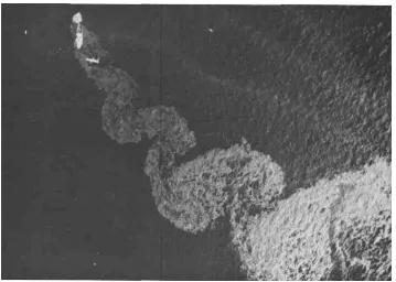
structures unique to shallow flows. An interesting case in this category is the crude oil
spill from the oil tanker Argo Merchant southeast of Nantuket Shoals, Massachusetts in
December, 1976 (Van Dyke, 1982). The shallow wake generated by the dispersion of the
crude oil in the sea water is observed clearly in the picture shown in Figure 1.2.
Tidal waves in shallow flow: In addition to atmospheric flows, the wake flow shed from
solid obstacles like bridge piers may be dangerous in some instances. One of these
instances is the tidal wake of Naruto Strait, which connects the Awaji and Shikoku
islands in Japan. The left picture in Figure 1.3 shows a freighter stranded in the tidal
wave below the bridge. The freighter got stranded in the whirlpool at around 11:00 AM
and remained so till the next high tide arrived. In the left picture, a whirlpool of diameter
approximately 15 m can be seen in the lower right corner. On the right picture, the
whirlpool can be seen very clearly.
Miscellaneous flows: Shallow flows can also be observed in air conditioning applications
(Kanda & Linden, 2003), plate heat exchangers and liquid metal sheet casting process.
An extreme and almost exact representation of shallow flow can be found in experiments
of falling soapfilms (Goldberg et al., 1997) where the bounding surface is almost
three-dimensional structures and will contain only two-three-dimensional turbulent motions and
hence represent shallow flow.
1.3Motivation
Since the early days of Prandtl, there has been an enormous amount of research
dedicated to the study of flows around bluff-bodies. The mechanism of vortex formation,
flow separation and fluid-structure interaction constitutes the greatest part of the
literature. Considering the overwhelming number of publications and research hours
dedicated to this topic, any new investigation seems to be redundant. But, given the
enormous importance of these flow features, it generates new challenges that require
better understanding of the fundamental principles that govern them. Additionally, the
continuous evolution of computational and experimental techniques provides new
perspectives to the same problem. One of the major developments in the area of
experimental fluid mechanics is the development of the particle imaging techniques,
which enables one to perform measurements in the spatial domain, therefore presenting
an unprecedented wealth of information. The combination of computational resources
with the development of the charged-coupled-device (CCD) makes the future of fluid
mechanics research more promising, especially for flows in which fluid-structures of
different scales co-exist.
The major contribution of the present study is to combine the available hardware,
software and mathematical tools for the exploration of the characteristics of a typical
use of the state-of-the-art particle image velocimetry technique to measure the spatial
characteristics of the shallow wake, use of modern techniques to evaluate and process the
measurements, development and application of recent mathematical techniques to educe
coherent structures in the flow.
Finally, one last paragraph is necessary to define the author’s motivation and
drive throughout the research. It is not only the complexity of the nature itself, but
complexity of the fluid mechanics that this work is intended to address. But what makes
our life far more complex is the human nature, our human curiosity that continuously
drives us to seek new challenges to overcome, new questions to answer and new obstacle
to overcome. We have reached a tremendous level of understanding of the nature
surrounding us, still it is highly appropriate to quote the great philosopher Aristotle
“….the more I understand, the more I realize the little I know”. Any scientific
investigation will end up posing new set of questions and obstacles to overcome. There is
no doubt that a dissertation is expected to resolve an issue in considerable depth so that it
can address almost all questions in mind. However, it will be arrogant to claim or expect
that the present investigation will come up with a complete solution of the problem we
are examining. In this circumstance, the major objective and personal ambition is to
develop versatility, problem solving ability and a broard understanding of the relevant
physics and the problem solving abilities. This is, of course, an endless process, but
laying the ground and the foundation upon which one can build and evolve these skills is
1.4Scope
A typical shallow wake was generated by immersing a sharp-edged bluff body in
a shallow open channel flow. The depth of flow was maintained nominally at 100 mm
and the aspect ratio of the flow was 12. The flow was subcritical and in turbulent state.
According to previous literature, the stability number of the wake implies negligible
effect of the bed. Particle image velocimetry measurement was carried out at near-bed,
mid-depth and near-surface locations ranging in the streamwise direction extending to ten
times the body width.
A general review of the available literature on shallow wake flow is presented in
Chapter 2. Following a brief introduction of turbulent flow, the source of uniqueness of
the shallow wake is explored. The literature is loosely classified based on the effect of
bed, free surface and the approaching flow. In light of the available literature, the
relevance of the present study is stressed at the end of this chapter. Chapter 3 contains the
description of the particle image velocimetry system used in the measurement. Since
particle image velocimetry is a recent technique, a brief introduction of the measurement
principle is illustrated and then the configuration of the present series of experiment is
discussed. Chapter 4 contains the discussion about the vertical variability of the wake
flow in terms of the mean velocity profiles and turbulence parameters at specific
streamwise locations at the near-wake region. The presence and effect of coherent
structures at the near-bed and near-surface region has been highlighted, but no
quantitative information is provided. Chapter 5 covers the vertical variability of the
time mean velocity, vorticity and turbulence parameters. The effect of the bed and the
free surface on the vorticity distribution is highlighted and a phenomenological picture of
the flow field is reconstructed. Chapter 6 concerns the application of the proper
orthogonal decomposition technique to decompose the flow field into coherent and
incoherent parts. The large-scale coherent structures are identified by a novel
closed-streamline based vortex identification scheme. Following the identification, a statistical
description of the location, size, sense of rotation and circulation of these structures are
documented as a step towards quantification of the shallowness effect on the large-scale
coherent structures. Lastly, the thesis ends by summarizing the conclusions and
recommending a possible path for future study. The related Matlab® scripts used for the
Figure 1.1: Vortex street of the Juan Fernandez Islands 1
Figure 1.3: Shallow wake in Naruto Strait and the ship stranded in the whirlpool2
Chapter 2
LITERATURE REVIEW
2.1General remarks
This chapter discusses the current state of development in the investigation of
shallow wake in open channel flow. Open channel flow itself has several unique features
and differs considerably from the conventional boundary layer like flows. Herein, open
channel flow is first discussed in brief, to provide the required details of the background
flow. According to the existing literature, the uniqueness of a shallow wake is determined
by three factors: the effect of bed, the effect of the free surface and the effect of the
nonuniform vertically sheared approaching flow. A major portion of the relevant
literature is discussed under these three subheadings. Some of the investigations that can
not be categorized under these headings are discussed in a separate subsection. The
chapter concludes by highlighting the importance of the present study.
2.2Introduction
Numerous flows occurring in nature can be regarded as shallow (Vriend, 2004).
In these flows, the length scale in the horizontal direction is much greater than that in the
vertical direction (Jirka & Uijttewaal, 2004). Examples of shallow flow can be found in
rivers, headlands, estuaries, stratified lakes and coastal seas (Vriend, 2004). Heat
dissipated from the earth can bring forth density variation in the vertical direction which
can induce shallow flow over mountains and hills (Scorer, 1978). Knowledge of the
predicting the flow, besides assisting in analyzing the dispersion of heat, pollutants and
biological species. Furthermore, it would also aid in weather modelling as the waterbeds
and marshlands play a crucial role in controlling the local weather condition (Jirka &
Uijttewaal, 2004).
From the perspective of fluid dynamics, shallow flow has important features due
to the presence of the bounding surfaces in the form of the bed and the free surface. The
bed imparts vertical shear while the free surface acts as a stress-free weak boundary. A
typical shallow wake can be generated by introducing a disturbance in the form of a
bluff-body in an otherwise plane flow. The resulting separation of flow from the sides of
the body, though similar to a deep wake, would be modified due to the effect of the
background flow conditions. As a first step, a brief discussion of a shallow channel flow
is necessary, as this constitutes the background flow condition for the shallow wake.
2.3Shallow channel flow
The simplest example of shallow flow is the plane uniform open channel flow.
This type of flow is unique because it developes under a confinement bounded by the
side walls of the channel and by the free surface which is subject to atmospheric pressure.
The flow is driven along the slope of the channel by the component of the weight of the
liquid, and the shear force on the channel boundaries is the main resisting force. Open
channel flows can be classified as shallow when the vertical length scale of the flow
(usually the depth, H) is significantly smaller than the horizontal/transverse length scales
(Jirka & Uijttewaal, 2004). While in the limit of infinite depth, flow in open channels
applications and hydraulic engineering practice, this approximation is violated due to the
finite shallow depth of the flow.
2.3.1Near-bed region
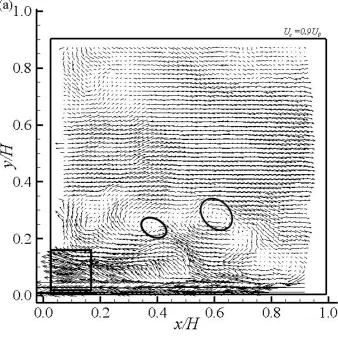
The shallow open channel flow is governed mostly by the wall turbulence. An
example of a velocity field in open channel flow obtained with the particle image
velocimetry (PIV) technique is shown in (a). This figure shows a typical time-averaged
velocity in a viewing window 100 mm long and 92 mm high. Averaging is done over
2000 PIV images. The mean velocity profiles conform to the typical pattern of the
streamwise velocity in wall-bounded flows. In many situations, the mean velocity can
still be characterized by the logarithmic law of the wall. However, recent experiments by
Pokrajac et al., (2007) in shallow open channel flows over rough beds have shown that
the logarithmic layer will form only if there is enough space between the top of the
roughness and the free surface. If this is not the case, the velocity profile may still have a
logarithmic shape, but the parameters of the corresponding logarithmic law may not have
the same physical meaning as the parameters of the universal logarithmic law of the wall.
One of the disadvantages of the time–averaging is that it hides much of the
unsteady features of the flow. In contrast, the instantaneous and fluctuating velocity
fields obtained at a particular instance. While the instantaneous velocity field ((b))
provides little evidence for the presence of vortical structures, the fluctuating velocity
field reveals well-defined patterns. In (c), a small vortex (highlighted by a circle) and a
of the same field can be seen. During the ejection event, fluid particles are lifted away
from the wall by the positive wall-normal fluctuations.
The structure of the turbulence in shallow open channel flows is
three-dimensional, dominated by ejection and sweep events. Near the bed, shallow open
channel flow is mainly occupied by fluid structures similar to these observed in the
turbulent boundary layer. Numerous studies have been devoted towards exploration of
the effect of the boundary layer in an effort to understand the associated dynamics of the
near-bed mechanisms (e.g., Falco, 1977; Head & Bandyopadhyay, 1981; Robinson, 1991;
Adrian, 2007). Mainly, the bed region is dominated by the negative streamwise
fluctuations with fluid particles being lifted away from the bed by positive bed-normal
fluctuations (ejection) and positive streamwise fluctuations moving towards the bed
(sweep). Above this region, turbulent bulges with a length scale of the order of
two-to-three wall units can be observed (Blackwelder & Kovasznay, 1972). In addition,
structures inclined about 45o to the bed, resembling a horseshoe, appear in the flow.
They are commonly known as hairpin vortices (Theodorsen, 1955). According to Kline
& Robinson (1989), the near-bed region is mainly occupied by the following structures:
low speed streamwise streaks in the viscous sublayer, events corresponding to ejection
and sweep, vortical structures of various forms, three-dimensional turbulent bulges and
hairpin vortices. Recent PIV measurements (Roussinova et al., 2008) in open channel
flow at shallow depth (H = 0.10 m) confirmed the presence of the hairpin vortices near
the bed. A simple way to visualize the vortical structures is to apply Galilean
field. This method is suitable for to uncovering vortices advecting at similar speeds.
However, in bounded flows, vortices advect with different speeds at different
wall-normal locations and, in order to reveal all embedded structures in the flow, one must
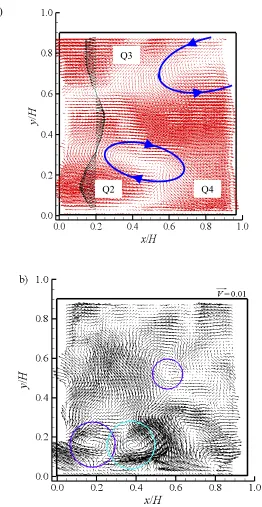
remove a broad range of advecting velocities. In Figure 2.2(a) and Figure 2.2(b),
Galilean decompositions of the instantaneous velocity field shown in Figure 2.1 are
presented. By removing different advection velocities from the instantaneous velocity
field, different structures can be seen. In Figure 2.2(a), several heads of the hairpin
vortices are visible with the circles moving in a frame convecting with UC = 0.9U0.
These vortices cannot be identified from the fluctuating velocity field shown in Figure
2.2. Figure 2.2(b) reveals the result of the Galilean transformation for a convection
velocity UC = 0.8U0. As the convection velocity becomes smaller than the maximum
velocity U0, the vortices near the solid wall become visible. More information related to
the existence of large-scale structures in the flow was presented by Roussinova et al.,
(2008) who applied the proper orthogonal decomposition (POD) technique to expose the
structures. Their POD results revealed the existence of hairpin vortices of different sizes
and energy levels. Further analysis of the POD reconstructed velocity maps was
performed using different combinations of modes to expose the energetic large-scale
structures, and less energetic small-scale structures. The first set of POD modes
recovered 50% of the turbulent kinetic energy while the second group of modes
recovered 33% of the kinetic energy. An example of a POD reconstructed velocity field
of recovering 50% of the energy is shown in Figure 2.3(a) where most of the large eddies
results also revealed patterns of strong ejection (Q2) and sweep (Q4) events which are
common features in wall-bounded flows. Close to the free surface, existence of hairpin
vortices was observed with legs possibly extended upwards towards the free surface.
Near the free surface, the induced flows from the large scale-structures contribute to the
increase of the quadrant 3 events. In Figure 2.3(b), POD reconstructed velocity field
from a second set of the POD modes recovering 33% of the energy is shown. By
combining the higher order POD modes (13-100), structures are exposed which appear to
be more circular. Hairpin vortices with length scales smaller or in the order of the flow
depth have been also found in shallow open channel flows (Nezu & Nakagawa, 1993).
Because of the shallow depth, most of the low speed fluid parcels often reach the
water surface, while at times still being attached to the bed. Nikora et al., (2007)
speculate that these low speed parcels can be viewed as clusters of fluid-made ‘cylinders’
randomly distributed in space and embedded into the faster moving surrounding flow.
These attached eddies can be responsible for weakening the horizontal eddies present in
the flow, providing for a very different mechanism of energy transfer.
2.3.2Near free surface region
Based on evidences put forward in the literature (e.g., Komori et al.; 1982, Willart
& Gharib, 1994, Maheo, 1999), close to the free surface the turbulent kinetic energy in
the vertical direction has been shown to be redistributed to the horizontal directions (both
streamwise and transverse). The redistribution of kinetic energy occurs in two separate
fluid layers close to the free surface (Hunt & Graham, 1978). The first layer is where the
component is enhanced. The second layer corresponds to a very thin viscous layer, where
the turbulent fluctuation of the vertical velocity rapidly diminishes to zero. Walker et al.
(1996) determined the thickness of the former and later layers to be approximately one
and one-tenth of the turbulent length scale, respectively. The energy redistribution is
limited to only large-scale structures of the flow, whereas the small-scale structures
maintain their universality. Based on these observations, Shen et al. (2000) proposed a
computational model for large-eddy simulation (LES) of free surface turbulence.
Close to the surface, mainly two types of structures can be observed; surface-
normal vortex tubes with predominantly vertical vorticity component and surface-parallel
vortex tubes buried inside the surface layer. Physically speaking, one would assume the
surface-normal vorticity would induce ‘pressure’ and control the deformation of the free
surface. But, Dommermuth (1994) concluded the presence of a weak correlation between
the free surface deformation and surface-normal vorticity by comparing the initial and the
final state of the vorticity induced pressure and the free surface deformation. The lack of
correlation is also supported by the findings of Zheng et al. (1999). However, Weigard &
Gharib (1995) performed simultaneous shadowgraph and PIV experiments to show that
the vertical vorticity location and strength correlate fairly well with the appearance of the
free surface deformation.
Due to the computational difficulty of modeling a free surface, very little
computational work was carried out until recently. The first direct numerical simulation
(DNS) of the free surface, utilizing the rigid lid assumption, was reported by Lam &
al., (1993) who utilized a full free surface computational model in the direct numerical
simulation. Pan & Banerjee (1995) performed DNS of open channel flow to explore the
large-scale structures appearing at the free surface. They broadly classified the structures
into three groups: ‘vortices’, ‘upwelling’ and ‘downdraft’. These types of structures have
also been reported by Gupta et al. (1994) based on experimental observations. ‘Vortices’
is the region of cluster of surface-normal vorticity where the ratio of surface-normal to
the surface-parallel velocity is close to zero, i.e., the vertical velocity towards the free
surface is negligible. ‘Upwelling’ is a region of divergence of streamlines with large
surface-normal velocity. The ‘downdraft’ region exhibits strong downward velocity
component originating from the free surface. It should be noted that the surface normal
velocity has to be zero exactly at the free surface, but these velocities mentioned above
are at a location of 10-20 wall units beneath the free surface, inside the surface layer.
When a typical upwelling reaches the free surface, a near circular vorticity pattern (donut
shaped) is generated. This pattern interacts with the free surface and generates vorticity
which connect with the free surface and form a number of short-lived vortices around the
edge of the upwelling. At the end of this cycle, downdraft takes place. The energy spectra
of the velocity close to the free surface shows k-5/3 and k-3.5 regions, which is
characteristic of two-dimensional turbulence, where k is the characteristic wave number.
The turbulent kinetic energy transfer spectra indicate flow of turbulent kinetic energy
from smaller to larger scales at the near-surface region. But at a considerable distance
from the free surface, deep within the flow, the usual three-dimensional turbulence
Nikora et al. (2007) used particle tracking velocimetry to explore the near-surface
structure of an open channel flow for both subcritical and supercritical flow conditions
(Froude number Fr = 5.64, 3.49 and 0.31; corresponding Reynolds number Red = 6437,
6397, 2736, respectively). Following the velocity measurement, the probability density
function, correlation function and structure function of the streamwise and transverse
velocity components close to the free surface were examined. These indicate the
existence of the large-scale structures of lateral extent larger then the flow depth at the
near free-surface location. The structures have characteristics that resemble
two-dimensional turbulence and depict inverse energy cascade. They postulated two possible
hypotheses regarding the appearance of the large-scale structures in shallow channel
flow. Any turbulent channel flow is characterized by sweep events and ejection of fluid
packets from the bed due to the associated dynamics of the turbulent boundary layer -
like region (Adrian, 2007). Due to the limited depth of shallow channel flow, these fluid
packets eventually arrive at the free surface while also being attached to the bed. One can
view these structures as a cluster of ‘fluid cylinders’ resembling tornadoes immersed in
the background flow. These structures interact with the instability associated with the
inflexion point of the transverse velocity distribution and generate horizontal structures
with two-dimensional turbulence characteristics. Another possible mechanism of
generation of these structures was put forward by Shen et al. (1999). The hairpin eddies
which are generated near the bed reach the free surface due to the limited depth of the
flow. In that situation, the head of the eddy quickly dissipates or is advected by the flow
It should be noted that a typical shallow turbulent channel flow contains
two-dimensional as well as two-dimensional structures. The length scale of the
three-dimensional structures ( ) is in the order of, or less than, the depth of flow. But the
two-dimensional structures of length scale ( ) greater than the flow depth, with
predominantly vertical vorticity is unique to shallow channel flow (Chen & Jirka, 1995).
Jirka & Uijttewaal (2004) has aptly summarized the following: “Shallow flows are
largely unidirectional, turbulent shear flows driven by piezometric gradient and
occurring in a confined layer of depth. This confinement leads to the separation of
turbulent motions between small scale, three-dimensional turbulence , and large
scale two-dimensional turbulent motion, l , with some mutual interaction.” D l3 D l2 H H l3D ≤
D ≥ 2
2.4Shallow wake
Before embarking upon the discussion of the shallow wake characteristics, a
convenient starting point may be a brief discussion of the deep wake. In this context, the
deep wake is defined as the wake produced when the body is immersed in a flow of
‘theoretically’ infinite depth, i.e., the approaching flow is uniform in nature and there are
no boundary effects. When any unbounded flow goes past a bluff body, four distinct
regions can be observed upstream and downstream of the bluff-body as mentioned by
Zdravkovich (1997). He broadly divided the field around the bluff body into four regions.
Region I is a very thin region of retarded flow directly upstream of the body. As the flow
impinges upon the body, a stagnation point is formed and a boundary layer is generated
region on the sides of the body, where the flow velocity is higher than the mean incoming
flow. This region is also called as accelerated flow region. Region IV is the region
directly downstream of the body and contains the recirculation region. Several aspects of
the deep wake including velocity defect profiles have been studied in detail (for example,
see Williamson, 1995, 1996). Usually, the incoming flow interacts with the boundary
layer formed on the body and the separated shear layer is shed as vortices in the
streamwise direction. Although, the vortex shedding process appears two-dimensional in
nature, there is considerable three-dimensionality in the flow (Wei & Smith, 1986). The
three-dimensionality mainly originates from the end condition (Ramberg, 1983) and may
induce spanwise disturbance and oblique vortex shedding (Hammache & Gharib, 1991).
In all cases, the separating boundary layer rolls up on both sides of the body and is
advected downstream as the von Karman vortex street. The periodic vortex shedding is
characterized by a nearly constant Strouhal number (St = fD/U ~ 0.2) for
. Important in the present context is the achievement of
self-similarity at far-wake streamwise locations (Pope, 2000).
000 , 100 Re
1000≤ D ≤
When a body is immersed in an open channel flow of finite flow depth, a shallow
wake is generated. The presence of the bounding surfaces (bed and free surface) has two
different effects on the development of a shallow wake as mentioned by Chen & Jirka
(1995). First, the limited depth restricts the onset of the three-dimensional breakdown of
the vortex street. As a result, the von Karman vortex street can be observed for a larger
range of Reynolds numbers in a shallow wake. For example, the pattern of crude oil
shows a clear vortex street pattern at a very high Reynolds number (Van Dyke,
1982). Secondly, the bed friction tends to arrest the transverse growth of the disturbances
associated with a typical vortex street pattern and stabilize the wake. This may occur
either in the near-wake, or in the far-wake region. For the case of a shallow wake, the
stability number, as will be shown later, determines the effect of the bed friction and the
subsequent wake stability. In the near-wake region, if the stability number
exceeds a certain critical value, wake stabilization takes place. In the
far-wake region, stability number is defined as
7 10 Re≈ H D C Snear = f /
H b C
Sfar = f2 / , where bis the local wake
width. Similar wake stabilization takes place at the far-wake region if exceeds a
certain critical value.
far S
2.4.1Stability number
Crucial to the development of the shallow wake is the mutual interaction of the
vertical shear due to the approaching flow with the horizontal (transverse) shear due to
the variation of momentum deficit in the transverse direction. Therefore, the
spatio-temporal growth of the shallow wake is controlled by their mutual interaction. The
shallow wake is maintained in an equilibrium state as a balance of two different effects:
on the one hand, turbulent kinetic energy is extracted from the mean flow and is fed to
the large-scale coherent structures by interaction with the lateral shear layer. On the other
hand, in the bottom boundary layer, the turbulent kinetic energy is extracted from the
large-scale structures and dissipated through the small-scale structures according to
energy due to the bottom friction by the production of the turbulent kinetic energy by the
lateral shear layer. The energy fed into the large-scale coherent structures can be
computed as the product of the coherent velocity fluctuations and the transverse mean
streamwise velocity gradient as (Babarutsi & Chu, 1985),
z U w u P c c
∂ ∂
= ; (2.1)
where, the subscript ‘c’ denotes the velocity associated with the coherent motions only.
and indicate the instantaneous velocity in streamwise (x) and transverse (z)
directions, respectively. The produced energy is dissipated through the small-scale
fluctuations at the bottom boundary layer. Babarutsi and Chu (1985) showed that if the
velocity associated with the coherent structure is small compared to the mean flow, then
the dissipation can be approximated as:
u w
) 2
(
2 c c c c
f
b U u u w w
H C
F = + , (2.2)
where Cf is the skin friction coefficient and H is the depth of flow.
Equating the above two equations, the flux stability number can be approximated as
c c c c c c f b
flux u u
w w u u z U H U C F P
S 2( )
2
+
∂ ∂ =
= . (2.3)
The ratio on the extreme right represents the ratio of the coherent Reynolds normal and
shear stress. Chu et al. (1983) proposed a gradient stability number for shallow flow,
2 2 y U ∂ ∂
= 0. Without affecting the calculation, the term at the extreme right can be dropped
safely and the velocity gradient can be expressed asΔU =U1 −U2, where U1 and U2 are
characteristic velocity at each side of the shear layer of local thickness δ. Thus, the
gradient stability number is
Inflexion f grad y U U H C S ∂ ∂ = H R C U U H
Cf δ avg f δ 2 = Δ
≈ ; (2.4)
where avg U U U U U U R 2 2 1 2
1 = Δ
+ −
= .
This equation is applicable for any general shear layer. For the case of a shallow wake, it
can be applied at the lee of the recirculation bubble. SinceU2 ≈0, R = 1 and the width of
the shear layer is approximated to be half of the diameter of the cylinder (D/2), the wake
gradient stability number can be found as,
H D C Sgrad f
4 1
= . (2.5)
The wake stability number (S) is four times the gradient stability number,
H D C S
S =4 grad = f . (2.6)
Unlike the gradient stability number, wake stability number (S) is a global parameter,
and it does not depend on the choice of local coordinate system. Therefore, it is a more
2.4.2Effect of the bed
As mentioned earlier, the uniqueness of a shallow wake depends on the combined
effect of the bed and the free surface. Although these two effects are closely interrelated,
it may be possible to view them independently. Wolonski et al. (1984) defined an island
wake parameter, , where Ua is the ambient flow velocity, H is the
flow depth, kz is the vertical eddy viscosity and D is the characteristic dimension in the
transverse direction. The vertical eddy viscosity was approximated as D
k H U
Pisland = a 2/ z
(
)
2 1 2 / 15 . 0 15 . 0 fz HU HU C
k = τ = , where is the friction velocity. They have
suggested that a critical value of Pisland of the order of unity exists, and a vortex street
type of wake is not possible for
τ
U
c P,island island
P < . Their classification is somewhat
incomplete and lacks descriptive information, as it is based on satellite imaging and
temperature mapping of the island wake and no direct measurements were conducted to
support the classification.
An important investigation in shallow wake was performed by Ingram & Chu
(1987) by observing the oceanic shallow wake behind island in Rupert Bay, Ontario.
Initially, they formulated an analytical description of the effect of the bed on the shallow
flow. To complement the formulation, they performed flow visualization in the
laboratory. A total of six laboratory observations and 26 events of oceanic shallow
wakes at Reynolds numbers (Re = 4HU/γ) ranging from 4,700 to 11,000, and stability
numbers ranging from 0.03 to 0.65 have been reported. They introduced the stability
of observations, they postulated a critical stability number of 0.48, above which the
oscillating characteristic of the wake gets stabilized due to the bottom friction. Below the
critical stability number, the effect of bed friction is not strong enough to stabilize the
wake and a vortex street type of wake can be observed. Figure 2.4 is adopted from their
paper and depicts three different cases; (a) Re = 11,000, Sw = 0.031, (b) Re = 11,000, Sw =
0.013 and (c) Re = 4,700, Sw = 0.054. Clearly seen in this figure is the suppression of the
wake oscillation with change in the Reynolds number and stability number. The frictional
effect of the bed is also shown to affect the entrainment coefficient of the wake.
However, the range of Reynolds number and stability number for the investigation is not
large enough to draw firm conclusions about the state of the wake.
Along the same lines, extensive laboratory experiments (57 with circular cylinder,
54 with solid plate and 34 with porous plate) and visualization of shallow wake was
performed by Chen & Jirka (1995) covering a wide range of Reynolds number and
stability number (Reh = 570-7300, Red = 3000-414000, S = 0.01-0.94). Based on visual
observations, they divided the shallow wake into three different categories: vortex street
type (VS), unsteady bubble wake (UB) and steady bubble wake (SB). If the perturbation
due to the separating shear layer is dominant, the shallow wake resembles the
well-known von Karman vortex street as seen in a conventional deep wake. Although
qualitatively similar, the vortex street of the shallow wake and the conventional von
Karman vortex street have significant differences. The vortex street (VS) shows a streaky
and fuzzy appearance due to the presence of the small-scale structures arising from the
roll up of the vortices. This type of wake is visible forS ≤0.2. If the stability number is
increased ( ), the bed friction effect increases and the flow separates from
both sides of the body simultaneously, not alternatively. A nearly steady bubble is formed
immediately downstream of the body. But the end of the bubble oscillates alternatively
and this leads to periodic breakdown of the vortices. This is called the unsteady bubble
(UB) wake. The steady bubble (SB) mode can be observed when the bed friction effect
decreases the momentum to such an extent that the recirculation bubble stays almost
stable at the lee of the body and no shedding is observed. By analytical approximation of
the wake momentum deficit, Chen & Jirka (1995) defined a length scale L beyond which
the wake momentum deficit disappears,
5 . 0 2
.
0 ≤S ≤
L= 2h/Cf = 2D/S.
Unstable shallow wakes get stabilized after a streamwise distance of the order of L,
mainly due to the increasing momentum deficit, and subsequent increase in the stability
parameter. They also observed that the width of the shallow wake greatly exceeds the
depth of the flow, and as a result the flow structures are mainly two-dimensional in
nature. They suggested that the majority of the effect of the bed friction is agglomerated
at the bottom boundary layer and may not contribute towards the three-dimensionality of
shallow flow. The bed friction effect is averaged over the full depth of flow and is
manifested in the form of the wake stability number.
Nagretti et al. (2005) mounted artificial roughness mats on the bed of a shallow
wake flow to investigate the effect of the increased roughness. Two series of experiments