Measurements and Modeling of Emissions, Dispersion and Dry Deposition of Ammonia from Swine Facilities

ABSTRACT

BAJWA, KANWARDEEP SINGH. Measurements and Modeling of Emissions, Dispersion and Dry Deposition of Ammonia from Swine Facilities. (Under the direction of Dr. Viney P. Aneja and Dr. S. Pal Arya).

Ammonia has recently gained importance for its increasing atmospheric concentrations and its role in the formation of aerosols. Studies have shown increasing

atmospheric concentration levels of NH3 and NH4+, especially in the regions of

MEASUREMENTS AND MODELING OF EMISSIONS, DISPERSION AND DRY

DEPOSITION OF AMMONIA FROM SWINE FACILITIES

by

KANWARDEEP SINGH BAJWA

A dissertation submitted to the Graduate Faculty of North Carolina State University

in partial fulfillment of the Requirements for the Degree of

Doctor of Philosophy

MARINE, EARTH AND ATMOSPHERIC SCIENCES

Raleigh

2006

APPROVED BY:

Sethu Raman Yang Zhang

Viney P. Aneja S. Pal Arya

Dedicated to My God

BIOGRAPHY

Kanwardeep Singh Bajwa was born on August 12, 1976, in his ancestral village Naserke, Punjab (India) to S. Hardev Singh and Mrs. Sukhwant Kaur. He spent his childhood in his village and did his schooling in Saint Francis Convent School, Fatehgarh Churian, a small town about 11 km from his village. Kanwardeep developed a deep interest in science and mathematics during his high school education. To pursue his interest in science, he joined as undergraduate student at Punjab Agricultural University (PAU) in Ludhiana, India. After completing his undergraduate studies in Agriculture with major in Horticulture, he joined MS in Agricultural Meteorology at Punjab Agricultural University. During his MS, he worked on a project “Wheat yield in relation to Western Disturbance Weather Systems in Punjab”. Kanwardeep was awarded with a merit scholarship for his excellent record in his studies at PAU. He successfully completed his MS in 2001. He also represented and won awards for his college and university as a part of folk dance (Bhangra) team at various national level competitions.

In the fall of 2002, Kanwardeep joined Air Quality Research Group at North Carolina State University to work Dr. Viney P. Aneja and Dr. S. Pal Arya as a doctoral student. While attending NCSU, he worked as a research assistant in the Department of Earth, Marine and Atmospheric Sciences. His doctoral research focused on ammonia emissions and deposition from swine facilities.

ACKNOWLEDGEMENTS

I owe a debt to “Almighty” with whose grace and blessings, I have been able to complete another chapter of my life. I am also indebted to my mother for her sacrifice, love, prayer and inspiration.

I feel pleasure to sincerely acknowledge co-chairs of my advisory committee, Dr. Viney P. Aneja and Dr. S. Pal Arya, for their patience, guidance and support throughout my doctorate studies. I would also like to thank my committee members Dr. Sethu Raman and Dr. Yang Zhang for their useful inputs during my research. I am very thankful to Dr. Deug-Soo Kim and Air Quality Research Group for all their help and support.

I am grateful to Dr. John Walker of USEPA and Matt Simpson of State Climate Office of North Carolina for technical discussions on my research. I would also like to thank Mark Yurka of North Carolina Division of Air Quality for his technical assistance on ammonia detection instruments and Brian Baldelli at Machine and Welding Purity Gases for his help in the delivering cylinders for field work.

Special thanks to my lovely wife “Ritu” for her love, patience, understanding and support throughout this period. Thanks for being a part of my life.

I would like to thank my family in India and Canada for their love, support and encouragement. Thanks to my niece and nephew Jass and Gary for their love. I am greatly indebted for ever-willing cooperation, help and moral support by my friends here in USA and in India. I want to thank my parents again for all their sacrifices and prayers for my success. I can never repay all they have done for me.

At last, I would like to thank North Carolina for all memorable times I have spent over here.

TABLE OF CONTENTS

List of Tables………... vii

List of Figures………viii

CHAPTER I

I

NTRODUCTION

1.1.1 Ammonia Emissions ……… …. 2

1.1.2 Ammonia Deposition……….. 5

1.2 Methods and Materials………..6

1.2.1 Dynamic Flow-Through Chamber system………6

1.2.2 Temperature Controlled Mobile Laboratory………...8

1.2.3 NH3 Detection Instrumentation………. 8

1.2.4 Meteorological Measurements………...9

1.2.5 Ambient Ammonia and Lagoon Parameters ……….. 9

1.2.6 Lagoon Sampling Scheme……….. 10

1.2.7 Automated Data Acquisition System……… 10

1.2.8 Ammonia Flux Calculation……… 10

1.2.9 Sampling sites ……… 12

1.3 Model Description ……….13

1.3.1 Two-film theory ………. 14

1.3.2 Simplified Diffusion Equation………... 15

1.3.3 Solution of Basic Diffusion Equation……… 15

1.3.4 Ammonia Flux……….17

1.3.5 Ammonia Flux with no Reactions (Equilibrium Model)………….17

1.3.6 Ammonia Flux with Reactions (Coupled mass transfer and chemical reactions model)………... 18

1.3.7 Mass Transfer Coefficients………... 19

1.3.8 Temperature Dependence……….. 20

1.4 AERMOD – Dispersion model………..21

1.5 Objectives………24

1.6 References………...25

CHAPTER II Measurement and Estimation of Ammonia Emissions From Lagoon-Atmosphere Interface using a Coupled Mass Transfer and Chemical Reactions Model, and an Equilibrium Model 2.1 Introduction………...40

2.2 Sampling and Measurement……….…… 42

2.2.1 Sampling Locations and Periods………... 42

2.2.2 Instrumentation and Measurements……….….... 42

2.3. Mass Transport models……….…... 44

2.3.1 Basic Diffusion Equation and its Solutions……….. 44

2.3.2 Equilibrium Model……….…… 46

2.4.1 Sensitivity Analysis of Equilibrium and Coupled Models……….. 48

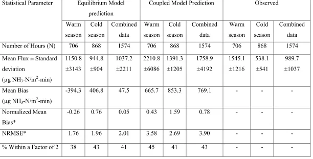
2.4.2 Comparison of Model Predictions with Observations……….49

2.4.3 Other Model Performance Statistics……….51

2.5. Conclusions……….…...53

2.6 References………... 56

CHAPTER III Modeling of Ammonia Dispersion and Dry Deposition studies at some Hog farms in North Carolina 3.1 Introduction………...68

3.2 Methods and Materials………..70

3.2.1 Measurements………. 72

3.2.2 Model simulations………... 72

3.3 Results and Discussions………. 73

3.3.1 Dry Deposition Velocity……….…….73

3.3.2 Dispersion of ammonia………..……. 75

3.3.3 Ammonia Deposition………..….... 78

3.4 Conclusions………... 82

3.5 References………..….... 84

CHAPTER IV Conclusions………97

APPENDICES……….. 101

Appendix 2 Abstract from paper submitted to Atmospheric Environmental... 103

Appendix 3 Abstract from paper submitted to Atmospheric Environmental... 104

Appendix 4 Abstract from paper submitted to Atmospheric Environmental... 106

Appendix 5 Abstract from paper submitted to Atmospheric Environmental... 108

Appendix 6 Abstract from Agricultural Air Quality: State of the Science…… 109

List of Tables

CHAPTER 1

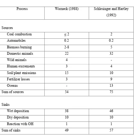
Table 1.1 Estimates of sources and sinks of ammonia (Tg year-1 as nitrogen)

(1Tg=1012)………... 30

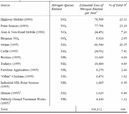
Table 1.2 Nitrogen emission inventory for North Carolina (NCDENR, 1999)…….31 Table 1.3 List of swine farms and measurement periods………...32

CHAPTER 2

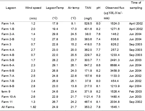
Table 2.1a Mean values of observed flux and other parameters during the

warm season………...59 Table 2.1b Mean values of observed flux and other parameters during the

cold season………. 60 Table 2.2 Statistical performance parameters for Equilibrium and

Coupled models………. 61

CHAPTER 3

Table 3.1 Comparison of modeled versus measured dry deposition velocities...88 Table 3.2a Dry deposition of ammonia (in grams and percentage) and related

parameters from Barham farm during the spring season measurement

period………... 89 Table 3.2b Dry deposition of ammonia (in grams and percentage) and related

parameters from Barham farm during the fall season measurement

period………. 90 Table 3.3a Dry deposition of ammonia (in grams and percentage) and related

parameters from Moores farm during the summer season measurement period………. 91 Table 3.3b Dry deposition of ammonia (in grams and percentage) and related

parameters from Moores farm during the winter season measurement

List of Figures

CHAPTER 1

Figure 1.1. Hog population and number of farms in North Carolina. (Source

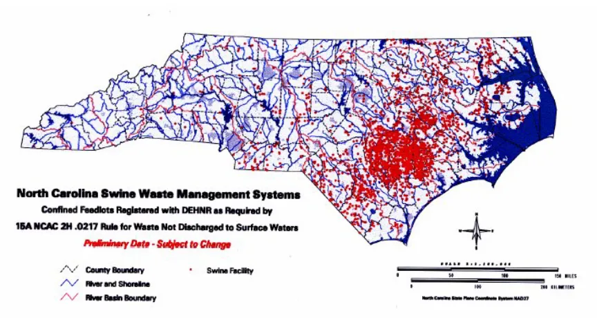
NCDENR, 1999)………...33 Figure 1.2. Swine distribution in North Carolina (Source Aneja et al., 2000)…….. 34 Figure 1.3 Ammonia flux measurement dynamic flow through chamber

system……….….. 35 Figure 1.4 Two film theory of mass transfer (Aneja et al., 2001b)……….….. 36 Figure 1.5 Data flow in the AERMOD modeling system (USEPA, 1998)………... 37 Figure 1.6 AERMET Processing (USEPA, 1998)...………..……38

CHAPTER 2

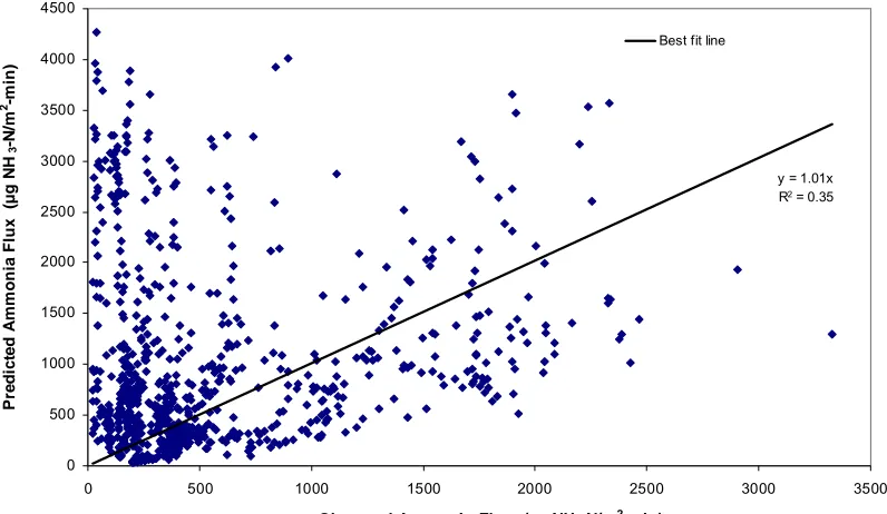
Figure 2.1 Schematic of mass transfer across liquid and gas film……….62 Figure 2.2a Comparison of Equilibrium model with observed ammonia flux data with a

best fit line for warm season (Some high flux data points are out of the scale shown here)………....63 Figure 2.2b Comparison of Equilibrium model with observed ammonia flux with best fit

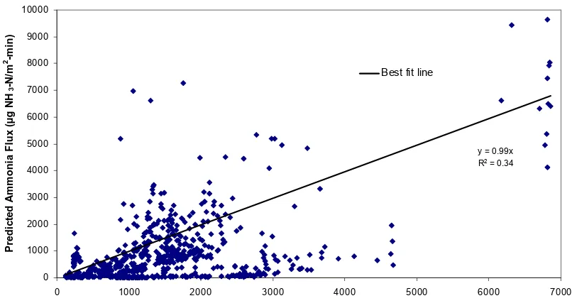
line in cold season………..…....64 Figure 2.3a Comparison of Coupled model with observed ammonia flux data with best fit

line for warm season (Some high flux data points are out of the scale shown here)………... 65 Figure 2.3b Comparison of Coupled model with observed ammonia flux with best fit line

in cold season………...66

CHAPTER 3

Figure 3.1 Orientations of Barham farm and Moores farm with respect to wind direction……… 93 Figure 3.2 Change in dimensionless ground-level concentration with dimensionless

distance for several stability conditions based on Zo/L at Barham farm with direction along the orientation 1………..….. 94 Figure 3.3 Normalized cross-wind integrated ground-level concentration as function of

normalized downwind distance, for convective conditions based on H/L at Barham farm with direction along the orientation 1………..95

Figure 3.4. Vertical profile of normalized cross-wind integrated concentration (C*) at

CHAPTER 1

I

NTRODUCTION

Ammonia is an important atmospheric pollutant that plays a key role in several air pollution problems. Ammonia in gaseous form is closely linked to the presence of ammonium in the atmosphere, which in turn acts as neutralizing agent in the atmosphere and also contributes to the regional acidification problems (Warneck, 1999). Ammonium

salts remain a major component of inorganic atmospheric aerosols and thus NHx (NHx =

ammonia + ammonium) plays a major role in the physical and chemical processes of the atmospheric nitrogen cycle. Ammonia is gaining increasing importance, as a principle source of atmospheric aerosols (Baek and Aneja, 2004). Ammonia also plays a role in formation of new particles by gas to particle conversion process. Oxidation of SO2 to H2SO4 and its neutralization by ammonia to form sulfate salts is an example of this process (Warneck, 1999).

Earlier, scientists believed that only importance of atmospheric ammonia was its role as source of fixed nitrogen to soil and plants. It was only in mid fifties that Junge (1954, 1956) recognized that ammonia is a single trace gas capable of neutralizing the

acids produced by the oxidation of SO2 and NO2 in the atmosphere. Ammonia reacts with

acidic atmospheric species, such as sulfuric acid, nitric acid and hydrochloric acid, to form ammonium aerosols, e.g., ammonium bisulfate, ammonium sulfate, ammonium

nitrate and ammonium chloride. Approximately 10% of the atmospheric NH3 also reacts

with hydroxyl radicals to form amide radicals (Finlayson Pitts and Pitts, 2000; McColloch et al., 1998).

in terrestrial ecosystems, effects that can result in the greater export of N to surface and groundwater (Paerl, 1995). Aber et al. (1989, 1998) hypothesized that high N inputs lead to “nitrogen saturation.” Saturation reduces the ability to assimilate and retain further N additions in an ecosystem. The result is an increased nitrate formation and its subsequent loss to surface and groundwater. The level of N input required to saturate an ecosystem will depend to a very large extent on the makeup of the community and will include many non-biotic factors related to the properties of the soil and climate. Ammonia can cause foliar injury to exposed plants, reduce growth and productivity, increase soil acidity and decrease biodiversity. In agricultural systems, addition of NO3- to soil (initially as NH3 or NH4+) and the consequent increases in emissions of N2O (nitrous oxide, a

greenhouse gas) and leaching of NO3-to the ground and the surface waters are of major

environmental concern (Krupa, 2003). North Carolina’s Albemarle-Pamlico Sound system is one of many North American, European and Asian estuarine and coastal ecosystems impacted by atmospheric nitrogen deposition which are exhibiting advance signs of eutrofication in form of recurring toxic and non-toxic phytoplankton blooms (Pearl, 1991, 1995; Paerl et al., 1993).

1.1.1 Ammonia Emissions

With the increasing human demand for food production, the use of nitrogen containing fertilizers and production of domestic livestock is increasing. Domestic animal waste is the major source of ammonia emissions. Estimates of global ammonia emissions budget indicate that domestic animal waste emits approximately 20 to 35 Tg of ammonia to the atmosphere per year, representing approximately half of the annual global ammonia emissions (Table 1.1). Other natural and anthropogenic ammonia sources, such as soils and biomass burning, contribute smaller portions to the global ammonia budget (Warneck, 1999).

Ammonia is increasing in importance in the rural atmosphere over the eastern United States (Aneja et al, 2001a, 2000). The number of commercial swine facilities in North Carolina has increased dramatically, with the state’s hog population increasing from approximately 2.8 million in 1990 to 9.8 million in 1997 when a moratorium on new hog farms was placed (Figure 1.1). Much of the increase in hog industry has occurred in coastal plane region, where more than 8.5 million hogs currently reside (Aneja et al., 2000) (Figure 1.2).

Measurements made at National Atmospheric Deposition Program and National Trends Networks sites in North Carolina show an increasing trend in the ammonium concentration in the precipitation since 1990 (Walker et al., 2000). This trend occurs in conjunction with an increase in the number of nearby swine operations. Coincident with the growth of swine numbers in the state, there has been a decline in the total number of farms raising swine (NCDENR, 1999) (Figure 1.1). The decrease in the total number of farms raising swine is the result of the closure and consolidation of small family farms and a move toward the industry preference of large farms that house more than 2,000 heads. The confined method of feeding and waste removal currently being used by the swine industry creates substantial quantities of anaerobic waste.

For reduction strategies to put in place, we need to know the total budget of ammonia and contribution of various sources. Such a task requires extensive field measurements and modeling. Table 1.2 gives us nitrogen emission inventory for North Carolina. Swine farms contribute to about 20% of nitrogen emissions. The major source of nitrogen from swine farms is ammonia. Different approaches have been made to quantify the ammonia emission sources.

and upper range of emissions vary from 100000 to 180000 Mg/year (Mg = 106g), which indicates a large uncertainty in ammonia emission estimates. Major uncertainties in emission estimates seem to be related to the use of simple emission factors, many of which are highly empirical or have been derived from measurements carried out under conditions which deviate considerably from those following modern practices of handling and applying manure and fertilizers (Schjorring, 1998).

Seventy five percent of swine production systems in North America and northern Europe use anaerobic or liquid/ slurry systems for waste holding, which is a major source of ammonia emissions (Safley et al., 1992). Emission rates from waste lagoons are difficult to measure, requiring specialized equipment and appropriate transport-measurement technology to obtain realistic emissions in relation to variable climatic and management conditions where animal production occurs. An emission model to predict ammonia emissions would reduce the expense of determining emissions on the large number of lagoons.

Measurements of ammonia flux from hog waste treatment lagoons (Aneja et al., 2001b; Aneja et al., 2000) and from fertilized and unfertilized soils (Roelle, 2001) have recently been made and analyzed with respect to corresponding environmental parameters, including lagoon and soil temperature, pH and total ammoniacal nitrogen (TAN).

Studies have also been done to model ammonia emissions. Previous studies have utilized theoretical models to study ammonia emissions from animal waste and soil. Koelliker and Minor (1973) developed a desorption model for ammonia emissions using two film theory. The overall mass transfer co-efficient (Halsem et al, 1924) in this model depends on wind velocity and temperature, and gives an emission of zero under calm conditions with no wind.

pits in swine buildings was done by Zhang et al. (1994). De Visscher et al. (2002) developed a two-layer model to study emissions from anaerobic lagoon. The model uses effluent concentration, water temperature, wind speed and effluent pH. It takes into account the aqueous equilibrium reaction of ammonia and ammonium, the adsorption of ammonium on the suspended organic material, and the diffusive transfer of ammonia and ammonium across liquid and air boundary layers.

Aneja et al. (2001b) developed a Coupled mass transfer and chemical reactions model and an Equilibrium model to simulate ammonia emissions from swine waste lagoons. Their two-layer models are based on the two-film theory using molecular transfer of ammonia across the lagoon-air interface. The Coupled mass transfer and chemical reactions model also takes into account pseudo-first order reaction of ammonia

with water and acidic species (H2SO4, HNO3, HCl) in the atmosphere. It incorporates air

temperature, lagoon temperature, pH, wind speed, TAN and ambient ammonia concentration. This model shows exponential increase with lagoon temperature and pH and linear increase with wind speed and TAN.

This study will include comparison of measured ammonia emission fluxes from swine waste treatment lagoon systems and modeled ammonia emission fluxes using the models developed by Aneja et al. (2001). Comparison of measured and modeled emission fluxes will help us to validate the models and also help us to make improvements in them and in measuring techniques of required parameters in this model.

1.1.2 Ammonia Deposition

NH3 emissions from source region, primarily evolving from swine and poultry

operations, are found to increase NH4+ concentration in precipitation at locations up to ~

80 km away (Walker et al., 2000). Poor et al., (2001) studied nitrogen deposition in Tampa Bay area. They found that 46% of nitrogen deposition occurs by dry deposition,

of which NH3 was a major contributor. Phillips (2003) showed that NH3 contributed 47%

of the total nitrogen dry deposited in the Neuse river watershed. NH3 contributes to roughly half of the total nitrogen deposition in Denmark, according to a study conducted by Howmand et al. (1993, 1994).

Results presented in NCDENR (1999) report demonstrate that ammonia emissions from swine production facilities can significantly enhance dry deposition of

NH4+-N to adjacent forest canopies. At the Eastern Farm site, NH4+-N dry deposition was

approximately two times (10.2 kg N/ha) that from wet deposition during the collection

period of August 6, 1997 to April 16, 1998. Total NH4+-N deposition to the forest floor

(from both wet and dry deposition) was 14.5 kg N/ha. The dry deposition of NH4+-N observed at the Eastern Farm site also enhanced the apparent dry deposition of chloride (Cl-) (9.2 kg Cl-/ha) and sulfate (SO4=) (17.1 kg SO4/ha).

Adverse effects on sensitive ecosystems caused by high N deposition can be reduced by lowering the emissions and, to a limited extent, also by removing sources close to the ecosystem to be protected (Asman et al., 1998b). This study has been selected to help develop an ammonia emission model from waste treatment lagoon that can be used to develop ammonia emission factors to study the transport of ammonia and its dry deposition downwind of the swine facilities taking one swine unit as a study model. We will also study dispersion and dry deposition of ammonia downwind of swine facilities,

to quantify ammonia concentrations downwind. As NH3 dry deposition velocity shows a

diurnal and seasonal variation (Phillips et al., 2004), we will study diurnal variation of ammonia along with seasonal variations.

1.2 Methods and Materials

1.2.1 Dynamic Flow-Through Chamber system

1988) was used to determine NH3 flux from lagoon surfaces (Figure 1.3). A translucent plastic cylindrical chamber of height 45.7 cm and diameter 25 cm (volume of 24.34 liter) was used. It was fitted in a circular hole cut in the center of a floating platform of 1.2 m × 1.2 m. The cylinder is fitted into the hole in the center of the platform, so that it penetrates into the lagoon surface by ~ 7 cm. The chamber was lined with a 5 mm thick fluorinated ethylene propylene (FEP) Teflon sheet throughout the inside surface of the chamber. Variable speed motor driven Teflon stirrer or impeller was used to mix the air inside the chamber. A carrier gas of compressed air travels into the chamber through a ¼ inch Teflon at a variable flow rate of 4-8 litre per minute (lpm) set by mass flow controller and monitored by a datalogger. The sample from the chamber travels through another ¼ inch Teflon tubing to the detection instrument. Teflon tubing and lining was used to minimize the chemical reaction with the sample stream. With the flow rate of 5 lpm, this equates to sample residence time of approximately 5 minutes in the system and 3 seconds in the lines at steady state. The vent in the sample line prevents the system from over pressurizing and was bubble tested periodically.

Air inside the chamber is well mixed with impeller speeds 40-60 rpm for this study. Roelle (1996) found that varying the speed of Teflon propeller within the above range did not produce any significant changes in the calculated NO soil flux using the chamber method. Johansson and Granat (1984) measured the pressure differences between outside atmosphere and air inside a chamber using a tilted water manometer.

They found that pressure differences were below detection limits (0.2 mm H2O). Bunton

(1999) conducted an experiment to explore possible differences between air temperature inside the chamber and ambient temperature. His study found maximum temperature

differences of 2.50C and 3.40C over two 24-hr experiments, which may have a minimal

1.2.2 Temperature Controlled Mobile Laboratory

The mobile laboratory used in our field measurements consists of a modified Ford Aerostar van with 13,500 BTU air conditioner unit. All the instrumentations are placed in this van. The temperature inside the van is regulated for effective performance of the ammonia analyzers. A 110 volt outlet was used to power the air conditioning and all detection instruments.

1.2.3 NH3 Detection Instrumentation

Thermo Environmental Instrument Incorporated (TECO) Model 17c chemiluminescnce ammonia analyzers were continuously used to monitor ammonia concentrations during ammonia flux measurement periods. Theory of working of this

instrument relies on high temperature catalytic conversion of NH3 to NO,

4NH3 + 5O2

→

and subsequent detection of NO based on the reaction between ozone and nitric oxide.

NO + O3

→

The photon produced in this reaction is detected by the photomultiplier tube converted into concentration of NO after calibration with known standards (TECO, 1999).

The sample stream entering analyzer is divided into 3 paths. The first path mixes the sample with ozone (O3), and all of the nitric oxide (NO) in the sample reacts with

ozone and give us nitrogen dioxide (NO2) concentration. Second path passes through a

molybdenum converter (325 oC) which converts all oxidized forms of nitrogen to nitric

oxide. This sample then reacts with ozone to quantify the concentration of all oxides of

nitrogen. Third sample line passes through stainless steel converter (750 oC) which

converts all nitrogen oxides and ammonia into nitric oxide, which gives total nitrogen

(NT). The sample stream alternates between three flow paths. Total ammonia is

temperature within that range. Further details of the TECO Model 17C ammonia analyzer and its calibration procedure are given by Philips et al. (2003).

1.2.4 Meteorological Measurements

A 10 m meteorological tower was erected at each site to measure wind speed and direction, temperature, relative humidity and solar radiation. A Met One Instruments Model 034B-L Windset was used to measure wind speed and direction at 10 m above the surface. This model consists of an integrated cup anemometer and wind vane. Accuracy of measured horizontal wind speed is ±0.12 m/s for wind speeds below 10.1 m/s and ±1.1% of reading for wind speed above 10.1 m/s. The horizontal wind direction has an

accuracy of ± 4o and a threshold of 0.4 m/s. Air temperature and relative humidity (RH)

measurements were made at a height of 2m facing north with a model HMP45C temperature and relative humidity probe housed in a radiation shield. RH accuracy is ±2

% (0-90% RH) and ±3% (90-100% RH) while air temperature accuracy is 0.2 – 0.5 oC.

Solar radiation measurements were also made at the 2m height but facing south using a model LI200X Silicon Pyranometer probe. Solar radiation has an absolute error in natural daylight of 5% maximum and 3% typical. (CSI Operator Manual Reference)

1.2.5 Ambient Ammonia and Lagoon Parameters

Ambient ammonia concentration was measured at 10 m height, using a filter with

1 m pores prevent the aerosols and dust particles to get in the instrument. Teflon tubes

were used to carry the sample to the ammonia analyzer. CSI Model 11-L50 Innovative

sensors pH probe continuously monitored lagoon pH during lagoon NH3 emission

measurement periods. Two C107 temperature probes measured lagoon temperature simultaneously inside the chamber and 0.5 m outside the chamber. Difference in lagoon temperatures inside and outside the chamber were found to be insignificant (less than

1oC). These pH and temperature probes were submerged in the lagoon at the depth of

1.2.6 Lagoon Sampling Scheme

Flux chamber was moved everyday in a random manner over the lagoon surface and Instruments were spanned everyday and flux chamber was flushed every time when it was moved to other part of the lagoon, to prevent the build up of ammonia in the chamber. Sampling locations were within 3m from the lagoon berm for easy access to the chamber without using a boat.

1.2.7 Automated Data Acquisition System

A Gateway laptop computer and a Campbell Scientific CR23X Datalogger (PC208W software) were used continuously collect data from all the instruments. It was placed in mobile laboratory. It stored data for ammonia from lagoon, lagoon temperature, lagoon pH, meteorological parameters and ambient ammonia. Data stored was averaged over 15 minutes. Data from datalogger was downloaded daily on laptop.

1.2.8 Ammonia Flux Calculation

The mass balance equation to calculate ammonia flux for the dynamic chamber system (Kaplan et al., 1988) is,

 

 

C

V

q

V

LA

V

JA

V

C

q

dt

dC













_















_



_-R

C NH3 concentration in a chamber (ppbv)

Cair NH3 concentration in ambient air (ppbv)

q Flow rate of compressed air through the chamber (lpm)

V Volume of chamber (24.34 liter)

A Surface area covered by chamber (m2)

Aw Inner surface area of the inner and upper wall surface of the chamber

L Total loss of ammonia in the chamber per unit area (m min-1) due to reaction with inner and upper walls of the chamber

h Internal height of the chamber

J Emission flux per unit area (µg NH3-N m-2 s-1)

R Rate of change due to reactions in gas phase

Zero air was used as a carrier gas, so that Cair is assumed to be zero. Since the chamber is assumed to be well mixed, concentration, C, is constant within the chamber. At steady state conditions, the change of concentration with respect to time will be zero. Also, since zero gas is used as a carrier gas, R is zero. With these conditions/assumptions, Eq (2) is simplified as:

eq w

_C

V

q

V

LA

h

J













_



Loss term L was determined experimentally while equilibrium-state ammonia

(Ceq), flow rate (q) and dimensions of the chamber (V and h) were all measured. Kaplan

et al. (1988) devised a method for calculating the loss term by determining the slope of the best-fitted line through a plot of























C

C

t

C

C

(

)

ln

versus time (t). For this experiment, Co is the initial equilibrium state NH3 concentration

measured by the chamber system at a constant flow rate of 12-14 lpm, Ceq is the

measured NH3 concentration at a second equilibrium state reached at a reduced flow rate

of 4-6 lpm into the chamber system, at C(t) denotes the NH3 concentration at any time, t,

_























_



w

A

V

V

q

slope

L

where Aw represents the area of the inner walls of the chamber.

1.2.9 Sampling sites

Ammonia flux measurements were made at swine facilities in south eastern North Carolina under the OPEN (Odor, Pathogens and Emissions of Nitrogen) project. Two of these sites employed Lagoon and Spray technology (LST) and others used potential Environmentally Superior Technologies (ESTs). At all the sites, measurements were made during two, two-week long periods, representing warm and cold seasons, respectively. The 2 LST farms and 9 EST farms used in this study are listed in Table 1.3 and are briefly described below. Their locations and measurement periods are given in Table 1.3.

Description of sites: (Table 1.3)

Stokes Farm is located near Trenton, NC, in Pitt County. Waste from the hog barns were flushed periodically (4 times a day) with recycled lagoon water and discharged into a storage pond from a single effluent pipe.

Moore Farm is located near Kinston, NC, in Jones County. Waste from all the hog barns was flushed out with recycled lagoon water and discharged into a storage pond from eight effluent pipes, one for each hog barn.

Brown’s of Carolina # 93 (EKOKAN) is located near Bladenboro, NC, in Bladen County. Biofilters are used to separate the solids from waste before it was pumped in lagoon.

Corbett # 1, 3, 4 (BEST: Solids separation/gasification for energy and ash recovery centralized system) are located near Rose Hill, NC, in Duplin County.

Howard farm (Constructed wetland system) is located in Onslow county. This project involves the utilization of constructed wetlands for effluent treatment following primary screening and solids separation.

Barham farm (In-Ground Ambient Temperature Anaerobic Digester System) is located near Clayton NC, in Johnston county. The ambient digester consists of an impermeable cover over an in-ground digester. Methane gas produced in this digester is used for electricity production at the site.

Harrell’s farm is located near Harrells, NC, in Sampson county. The permeable cover used is the Bio-Cap ML, designed to reduce ammonia emissions and odor.

Hunt farm is located near Wilson NC, in Edgecombe county. Pulverizer Air Dryer (PAD) technology is to be used to separate the solid and liquid portions of the waste stream from swine farms and dry the solid portion.

Carroll’s farm is located near Warsaw NC, in Duplin county. Waste flows first to what is described as a covered anaerobic pond; however, the cover is a layer of aerated water sprayed over the top of the pond. This aerated layer is designed to reduce ammonia emissions and odor. Wastewater then flows to an aerated nitrification pond and finally to a denitfication/irrigation storage pond.

Vestal farm is located near Kenansville NC, in Duplin county. This farm employs a mesophilic digester as well as aeration and a wastewater filtering and disinfection systems.

1.3 Model Description

The process of the conversion of ammonia in the atmosphere is a complex one involing various reactions, whose direction and rate are determined by atmospheric factors like relative humidity, pH and temperature etc. Most of the gaseous ammonia

(~90%, Aneja et al., 1997) in the troposphere is converted into NH4+ aerosols by reaction

of ammonia with sulfuric acid and hydrochloric acid. The following gas(g), liquid(l) and

solid (s). phase reactions summarize NH4+ aerosol production (Finlayson-Pitts and Pitts,

NH3 (g) + H2SO4 (l) → NH4HSO4 (l) NH4HSO4 (l) + NH3→ (NH4)2SO4 (l, s) NH3 (g) + HNO3(g) → NH4NO3 (s) NH3 (g) + HCl (g) → NH4Cl (s) NH3 (g) + H2O (l) → NH4+ + OH

-Ammonium aerosols return to the ground by dry and wet deposition processes. Tropospheric life of ammonia is less than 5 days, so it is removed in the region of its source itself (~80 km). Walker (1998) suggested that in North Carolina, the source may impact the distances of approximately 80 km depending on the wind direction.

Additional losses (~10%, Aneja et al., 1997) of ammonia are attributable to reactions of ammonia with hydroxyl radical (lifetime ~ 165 days, Warneck, 1988):

NH3 + OH → NH2 + H2O

1.3.1 Two-film theory

The principle characteristic of this two-film transport model (Figure 1.4) is an air-liquid interface for the exchange between water and air (Whitman, 1923, Cussler 1996). The interface between the two phases is a boundary between the two fluid layers. Each layer is a laminar surface layer of thickness ti (for liquid phase ti = tL and for air ti = ta) extending from air-liquid interface and to a well-mixed (turbulent) region in the interior of the lagoon and atmosphere, respectively. All the resistance to mass transfer across the interface is due to the layer in which transport is by molecular processes.

Reaction rate for the chemical reaction in the liquid and gas phase, in general, will depend on the local concentration of the gas, any other reactant with which it reacts, and other physical factors such as temperature and pH. The background concentrations of reactants in chemical processes in the liquid and gas phase involving ammonia do not

have significant variations. The ammonia concentrations CL and Ca at the other boundary

1.3.2 Simplified Diffusion Equation

Considering an element of differential thickness dz in the vertical direction with the unit cross sectional area, diffusion equation can be simplified as

 

C d

D_{i } _ri

    

2 2

(4)

where C is ammonia concentration, kri is the reaction constant in the phase I, Di = DL and

kri = krl for liquid and Di = Da and kri = kra for air, respectively. This equation follows directly from the basic advection equation, given by Arya (1999), after the assumption of steady state and horizontal homogeneity of flow and concentration fields are made.

1.3.3 Solution of Basic Diffusion Equation

Eq. 4 is a differential equation of second order whose general solution is (Malik, 1999),

C(z) = Aer×z + Be-r×z (5)

where,

i ri

D k

r and subscript i can be read as L for liquid and a for air.

Boundary Conditions:

LIQUID PHASE

z = 0; CL(0) = CL

z = tL; CL(tL) = CLi (6)

GAS PHASE

z = 0; Ca(0) = Cai

z = ta; Ca(ta) = Ca (7)

SOLUTION IN LIQUID PHASE;

Applying the boundary conditions in liquid phase, one can determine A and B in Eq. 5 as

L Lt

r L

Li

C

e

C

A







L L L L L L t r t r Li t r L

e

e

C

e

C

B







Substituting for A and B in Eq. (5), one obtains









e

e

e

e

C

e

e

C

C











( for 0 < z ≤ tL (10)

Where rL = ( krL/DL)1/2, krL is the overall reaction rate constant for reactions of ammonia

in the liquid, and DL is the diffusivity of ammonia in liquid phase.

SOLUTION IN THE GAS PHASE

Similarly equation can be solved for gas phase and solution to eq. (5) with boundary conditions in gas phase are as follows,









( for 0 < z ≤ ta (11)

where ra = (kra/Da)1/2

kra is an overall rate constant for ammonia reactions in gas phase (s-1), and Da is diffusivity of ammonia in the air (cm2/sec).

Cai and CLi are related by the henry’s law constant as,

Cai = HCLi (12)

Another boundary condition to solve the above equations is that fluxes at interface are equal

J = -DL (dC/dz) at z = tL, in liquid phase

This leads to the following expression for CLi,

CLi =

) )( ( ) )( ( ) ( 2 ) ( 2 L L L a a a a L L L a a a a a a a a L L L L t r t r t r t r L L t r t r t r t r a a t r t r L L L t r t r a a a e e e e r D e e e e r HD e e r C D e e r C D                       (14)

1.3.4 Ammonia Flux

Ammonia flux J is the diffusion flux at top of the air film and it is determined by the following relationship at the interface of the air film and turbulent region,

J = -Da (dC/dz) at z = ta (15)

Using equation (11) with z = ta and Cai = HCLi, one obtains the following expression for

the vertical ammonia flux:

J = Da ra (

a a a a a a a a t r t r Li t r t r a e e C H e e C     

 ) 2

(

) (16)

1.3.5 Ammonia Flux with no Reactions (Equilibrium Model)

Equation (16) is an expression of flux considering chemical reactions of ammonia in the liquid and air films. If we consider negligible chemical reactions in the liquid and air films, this expression should reduce to the form of equilibrium equation,

J = - K(Ca- HCL) (17)

where K = 1/(H/kL + 1/ka), is the overall mass transfer coefficient (m/s).

1.3.6 Ammonia Flux with Reactions (Coupled mass transfer and chemical reactions

model)

In order to determine the coupled transport and chemical reaction ammonia flux, we have considered ammonia’s reversible reactions in the solution and forward reactions only in the atmosphere. We can therefore determine the overall reaction rate for reactions of the ammonia in the atmosphere as follows,

NH3 + H2SO4 (l)

→

NH3 + HNO3(g)

→

NH3 + HCl (g)

→

NH3 + H2O (l)

→

-Above equation leads to the following relationship,

d[NH3]/dt = ( kH2SO4 [H2SO4] + kHNO3 [HNO3] + kHCl [HCl] + kOH [OH] ) * [NH3] and the reaction rate,

kra = kH2SO4 [H2SO4] + kHNO3 [HNO3] + kHCl [HCl] + kOH [OH] (18)

However since ammonia’s reaction in the liquid phase is reversible, the overall reaction rate will depend on the direction of the reaction. Olander (1960) has given the equations for predicting the effect of various types of equilibrium chemical reactions considering simultaneous mass transfer and equilibrium chemical reactions. Ammonia’s reaction in the solution is as below,

NH3(aq) + H2O ↔ NH4+ + OH

-Solution for CLi is obtained as,

CLi =

) ] [ D D + (1 ) ( HD ) ] [ D D + (1 2 L NH4 a L NH4 OH K t D e e e e r OH K t D C e e r C D L L L t r t r t r t r a L L L L t r t r a a a a a a a a a a a a a a a               (19)

1.3.7 Mass Transfer Coefficients

Halsam et al. (1924), Mackey and Yeon (1983), and Ibusuki and Aneja (1984), have determined the mass transfer coefficients. Mass transfer equations by Halsam et al. (1924) gives zero flux values at wind speed of zero. Mackey and Yeon (1983) used 11 hydrocarbon compounds of varying Henry’s law constant. They have empirically correlated the mass transfer coefficients in terms of friction velocity and Schmidt number. The empirical values of the mass transfer coefficients in air and water arrived by Mackey and Yeon are given below,

Mass transfer coefficient (in m/s) for the air,

ka = 1× 10-3 + 46.2 × 10-3 U * Sca -2/3 (20) where U* is friction velocity in m/s.

Mass transfer coefficient (in m/s) for the water,

kL = 1 × 10-6 + 34.1 × 10-4 U* ScL-1/2 (for U* > 0.3) (21) kL = 1×10-6 + 144 * 10-4 U*2.2ScL-1/2 (for U* < 0.3) (22)

Schmidt number (Sca and ScL) is the ratio of diffusion coefficient of ammonia to

kinetic viscosity for respective medium (air or water). These mass transfer coefficients provide more realistic estimates at zero wind speed, which is not the case with other studies.

of 0.01 R and 0.01 R (R= radius of droplet) are used for fast and slow aqueous kinetics reaction rates of the gas species. We have used Mackey and Yeon (1983) mass transfer coefficients for calculations in the equilibrium model.

1.3.8 Temperature Dependence

Density of ammonia in water and air are dependent on temperature of aqueous solution and air. Density and dynamic viscosity of water and air are related to the temperature of water and air respectively as per relationship provided by CRC 1989-90. Kinetic viscosity is the dynamic viscosity divided by the density. Diffusivity of water and air were used from Cussler (1996) as follows,

Dw =

25 25 298 ) 273 (     

 T_{L T}

D

(23)

where,

Dw and D25 are diffusivity at lagoon temperature and 25oC, respectively.

µT and µ25 are dynamic viscosity at lagoon temperature and 25oC, respectively.

Da =





m1= molecular weight of ammonia = 17g

m2= molecular weight of air = 29g

P = 1 atmosphere

V11 = diffusion volume of ammonia = 14.9 (at 1 atm)

V12= diffusion volume of air = 20.1 (at atm)

Henry’s law coefficient for flux equation is adopted from Hales and Drewes (1979) and related with lagoon temperature with the following relations,

1.4 AERMOD – Dispersion model

AERMOD (AERMIC Dispersion Model) model is designed to support the EPA's regulatory modeling programs to study short range dispersion and dry deposition. It was developed to replace ISC3 (Industrial Source Complex) dispersion model.

AERMOD is a steady-state plume model (USEPA, 1998). In the stable boundary layer (SBL), it assumes the concentration distribution in a continuous source plume to be Gaussian in both the vertical and horizontal. In the convective boundary layer (CBL), the horizontal distribution on the plume is also assumed to be Gaussian, but the vertical distribution is described with a bi-Gaussian probability density function (pdf). Additionally, in the CBL, AERMOD treats “plume lofting,” whereby a portion of plume mass, released from a buoyant source, rises to and remains near the top of the boundary layer before becoming mixed into the CBL. AERMOD also tracks any plume mass that penetrates into the elevated stable layer, and then allows it to re-enter the boundary layer when and if appropriate. For sources in both the CBL and the SBL AERMOD treats the enhancement of lateral dispersion resulting from plume meander.

Using a relatively simple approach, AERMOD incorporates current concepts about flow and dispersion in complex terrain. Where appropriate the plume is modeled as either impacting and/or following the terrain. This approach has been designed to be physically realistic and simple to implement while avoiding the need to distinguish among simple, intermediate and complex terrain, as required by other regulatory models. As a result, AERMOD removes the need for defining complex terrain regimes. All terrain is handled in a consistent and continuous manner while considering the dividing streamline concept in stably stratified conditions.

only a single surface measurement of wind speed (measured between 7 zo and 100 m,

where zo is the surface roughness height), wind direction and ambient temperature. Like

ISC3, AERMOD also needs observed cloud cover. However, if cloud cover is not available (e.g., from an on-site monitoring program) two vertical measurements of temperature (typically at 2 and 10 meters), and a measurement of solar radiation can be substituted. A full morning upper air sounding is required in order to calculate the convective mixing height throughout the day. Surface characteristics (surface roughness, Bowen ratio, and albedo) are also needed in order to construct similarity profiles of the relevant PBL parameters. AERMOD accounts for the vertical inhomogeneity of the PBL in its dispersion calculations. This is accomplished by "averaging" the parameters of the actual PBL into "effective" parameters of an equivalent homogeneous PBL.

Figure 1.5 shows the flow and processing of information in AERMOD. The modeling system consists of one main program (AERMOD) and two pre-processors, AERMET (AERMOD Meteorological Preprocessor) and AERMAP (AERMOD Terrain Preprocessor). The major purpose of AERMET is to calculate boundary layer parameters for use by AERMOD. The meteorological INTERFACE, internal to AERMOD, uses these parameters to generate profiles of the needed meteorological variables. In addition, AERMET passes all meteorological observations to AERMOD.

The AERMET is the meteorological preprocessor for the AERMOD. Input data can come from hourly cloud cover observations, surface meteorological observations and morning upper air soundings. Output includes surface meteorological observations and parameters and vertical profiles of several atmospheric parameters. AERMET is designed to be run as a three-stage process (Figure 1.6) and operate on three types of data --National Weather Service (NWS) hourly surface observations, NWS twice-daily upper air soundings, and data collected from an on-site measurement program such as from an instrumented tower. The first stage extracts (retrieves) data and assesses data quality. The second stage combines (merges) the available data for 24-hour periods and writes these data to an intermediate file. The third and final stage reads the merged data file and develops the necessary boundary layer parameters for dispersion calculations by

AERMOD. AERMET then calculates the PBL parameters: friction velocity (u*),

(zi), and surface heat flux (H). These parameters are then passed on to the INTERFACE (which is within AERMOD) where similarity expressions (in conjunction with measurements) are used to calculate vertical profiles of wind speed (u), lateral and vertical turbulent fluctuations (Fv, Fw), potential temperature gradient (dθ/dz), and potential temperature (θ).

The AERMAP is a terrain preprocessor designed to simplify and standardize the input of terrain data for the AERMOD. Input data include receptor terrain elevation data. The terrain data may be in the form of digital terrain data that is available from the U.S. Geological Survey. Output includes, for each receptor, location and height scale, which are elevations used for the computation of air flow around hills. In present study, we assumed flat rural terrain. So AERMAP will not be used in this study.

The model is capable of handling multiple sources, including point, volume, and area source types. Line sources may also be modeled as a string of volume sources or as elongated area sources. Several source groups may be specified in a single run, with the source contributions combined for each group. Source emission rates can be treated as constant throughout the modeling period, or may be varied by month, season, hour-of-day, or other optional periods of variation. These variable emission rate factors may be specified for a single source or for a group of sources.

The AERMOD model has considerable flexibility in the specification of receptor locations. The user has the capability of specifying multiple receptor networks in a single run. The user can input elevated receptor heights in order to model the effects of terrain above (or below) stack base, and may also specify receptor elevations above ground level to model flagpole receptors. There is no distinction in AERMOD between elevated terrain below release height and terrain above release height, as with earlier regulatory models that distinguished between simple terrain and complex terrain. For applications involving elevated terrain, the user must also input a hill height scale along with the receptor elevation.

Fd = C × Vd (26)

where

Fd = dry deposition flux (μg/m2/s),

C = concentration (μg/m3), calculated at reference height, zr,

Vd = deposition velocity (m/s)

The dry deposition flux is calculated on an hourly basis, and summed to obtain the total flux for the user-specified period. The default output units for dry deposition

flux in AERMOD are g/m2. Deposition velocity of gases is calculated as

Vd= 1/(Ra + Rb + Rc) (27) where

Ra = Aerodynamic resistance (s/m)

Rb = Quasilaminar resistance for bulk surface (s/m)

Rc = Bulk surface resistance (s/m)

1.5 Objectives

The primary objectives of this research initiative are:

1) Measurement of ammonia flux from swine waste treatment lagoons from facilities in South Eastern North Carolina using flux chamber system.

2) Validate the coupled mass transfer and chemical reaction model using the ammonia flux measurements from swine waste treatment lagoons.

3) To study the downwind short range dispersion of ammonia using US EPA’s regulatory short range dispersion model, AERMOD, with respect to different times of the day, meteorological conditions and season.

1.6 References

Aber, J.D., Nadelhoffer, K.J., Steudler, P., and Melillo, J.M., 1989. Nitrogen saturation in northern forest ecosystems: hypotheses and implications. Bioscience, 39, 378-386.

Aber, J.D.W., McDowell, K., Nadelhoffer, A., Magill, G., Berntson, M., Kamakea, S., McNulty, W., Currie, L., and Fernandez, I., 1998. Nitrogen saturation in temperate forest ecosystems: Hypotheses revisited. Bioscience, 48, 921-934. Aneja, V.P., Chauhan, J. P., and Walker, J., 2000. Characterization of atmospheric

ammonia emissions from swine waste storage and treatment lagoons. Journal of Geophysical Research (Atmosphere), 105, 11535-11545.

Aneja, V.P., Li, Y., and Walker, J.T., 1997. Atmospheric ammonia/nitrogen compounds emission and characterization” Workshop on Atmospheric Compounds Emission, Transport and Assessment. Sponsored by NCDENHR March 10-12, 1997 at NCSU, Raleigh, NC, 232-242.

Aneja, V. P., Malik, B.P., Tong, Q., Kang, D., and Overton, J.H., 2001b. Measurement and modeling of ammonia emissions at waste treatment lagoon-Atmospheric Interface. Water, Air and Soil pollution: Focus 1, 177-188.

Aneja, V. P., Murray, G., and Southerland, J., 1998. ‘Proceedings of the workshop on Atmospheric Nitrogen Compounds: Emissions, Transport, Transformation, Deposition and Assessment. North Carolina State University, Raleigh, NC, 299pp.

Aneja, V.P., Roelle, P.A., Murry, G.C., Souterland, J., Erisman, J.W., Fowler, D., Asman, W.A.H., and Patni, N., 2001a. Atmospheric nitrogen compounds II: emissions, transport, transformation, deposition and assessment. Atmospheric Environment, 35, 1903-1911.

Arya, S.P., 1999. Air pollution meteorology and dispersion. Oxford University Press, New York.

Asman, W.A.H., Sutton, M.A., and Schjorring, J.K., 1998b. Ammonia: Emission, Atmospheric transport and deposition. New Phytologist, 139 (1), 27-48.

Baek, B.H., Aneja, V.P., and Tong, Q., 2004, Chemical coupling between ammonia, acid gases, and fine particles. Environmental Pollution, vol. 129, 89-98.

Battye, R., Battye, W., Overcash, C., and Fudge, S., 1994. Development and selection of ammonia factors. EPA/600/R-94/190, Final Report Prepared for US Environmental Protection Agency, Office of Research and Development, EPA Contract No. 68-D3-0034, Work Assignment 0–3.

Battye, W., Aneja, V.P., and Roelle, P.A., 2003. Evaluation and improvement of ammonia emissions inventories. Atmospheric Environment, 37, 3873-3883.

Bunton, B.J., 1999. Measurement and analysis of atmospheric ammonia emissions from anaerobic lagoons. MS Thesis, North Carolina state University, Raleigh, NC. Chauhan, J.P., 1999. Characterization of the ammonia emissions from swine waste

storage and treatment lagoons. MS thesis, North Carolina State University, Raleigh, NC

Cussler, E.L. 1996. Diffusion: Mass transfer in fluid systems. Cambridge University Press, New York, NY.

CRC, (1989-1990). Handbook of Chemistry and Physics. Chemical Rubber Company Press, Cleveland, Ohio.

De Visscher A, Harper, L.A., Westerman, P.W, Liang, Z., Arogo, J., Sharpe, R.R., and Van Cleemput, O., 2002. Ammonia emissions from anaerobic swine lagoons: Model development. Journal of Applied Meteorology, 41, 426-433.

Finlayson-Pitts, B.J., and Pitts J.N., 1986. Atmospheric Chemistry. Wiley-Interscience, New York, NY.

Finlayson-Pitts, B.J., and Pitts J.N. Jr., 2000. Chemistry of Upper and Lower Atmosphere: Theory, Experiments and Applications. Academic Press, San Diego, CA.

Hales, J.M., and Drewes, D.R., 1979. Solubility of ammonia in water at low concentrations. Atmospheric Environment 13, 1133-1147.

Hanson, P.J., and Lindberg, S.E., 1991. Dry deposition of reactive nitrogen compounds: A Review of leaf, canopy and non-foliar measurements. Atmospheric Environment, 25A, 1615-1634.

Ibusaki, T., and Aneja, V.P., 1984. Mass transfer of NH3 into water at environmental concentrations. Chemical Engineering Science, 39, 1143-1155.

Jayaweera, G.R., and Mikkelsen, D.S., 1990. Ammonia volatilization from flooded soil systems: A computer Model, I. Theoretical aspects. American Journal of Soil Science Society, 54, 1447-1455.

Johansson, C., and Granat, L., 1984. Emission of nitric oxide from arable land. Tellus, 36B, 25-37.

Junge, 1954. The chemical composition of Atmospheric Aerosols, Measurements at Round Hill Field Stations June-July 1953. Journal of Meteorology, 11, 223-233. Junge, 1956. Recent investigations in Air Chemistry. Tellus, 8, 127-139.

Kaplan, W.A., Wofsy S.C., Keller, M., and Costa, J.M.D., 1988. Emission of nitric oxide and deposition of ozone in a tropical forest system. Journal of Geophysical Research, 93, 1389-1395.

Kim, D.S., Aneja, V.P., and Robarge, W.P., 1994. Characterization of nitrogen oxide fluxes from soils of fallow fields in the coastal piedmont of North Carolina. Atmospheric Environment, 28, 1129-1137.

Koelliker, J.K., and Minor, J.R., 1973. Desorption of ammonia from anaerobic lagoons. Transanction of ASAE, 148-151.

Krupa, S.V., 2003. Effects of atmospheric ammonia (NH3) on terrestrial vegetation: a review. Environmental Pollution, 124, 179-221.

Mackey, D., and Yeon, T.K., 1983. Mass transfer coefficients for volatilization of organic solutes from water. Environmental Science Technology, 17, 211-216.

McColloch, R.B., Few, G.S., Murray Jr. G.C., and Aneja, V.P., 1998. Analysis of Ammonia, Ammonium Aerosols, and Acid Gases in the Atmosphere at a commercial Hog Farm in Eastern North Carolina, USA. Environmental Pollution, 102, 263-268.

North Carolina Department of Environment and Natural Resources (NCDENR), 1999. Division of Air Quality, Status report on emissions and deposition of atmospheric nitrogen compounds from animal production in North Carolina. June 7, 1999, Raleigh, NC.

Olander, D.R., 1960. Simultaneous mass transfer and equilibrium chemical reaction, American Institute of Chemical Engineers Journal, 6(2), 233-239.

Olsen, J.E., and Sommer, S.G., 1993. Modeling effects of wind speed and surface cover on ammonia volatilization from stored pig slurry. Atmospheric Environment, 27A (16), 2567-2574.

Paerl, H.W., 1991. Ecophysiological and trophic implications of light stimulated amino acid utilization in marine picoplankton. Applied Environmental Microbiology, 57, 573-479.

Paerl, H.W., 1995. Coastal eutrophication in relation to atmospheric nitrogen deposition: current perspectives. Ophelia, 41, 237-259.

Paerl, H.W., Fogel, M.L., Bates, P.W., O’Donell, P.M., 1993. Atmospheric nitrogen deposition to estuarine and coastal waters: is there a link to eutrophication? In: Dyer, K (Ed.) Changes in fluxes to Estuarine implications from Science to Management. Olsen and Olsen, Copenhagen.

Philips, S.B., Arya, S.P., and Aneja, V.P., 2004. Ammonia flux and dry deposition velocity from near-surface concentration gradient measurements over a grass surface in North Carolina. Atmospheric Environment, 38, 3469-3480.

Phillips, S. B. 2003. Measurements, Modeling, and Analysis of Fluxes of Nitrogen Compounds. PhD Thesis, North Carolina State University, Raleigh.

Roelle, P.A. 1996. Oxidized and reduced biogenic nitrogen compound emissions into the rural troposphere: Characterization and modeling. PhD thesis, North Carolina State University, Raleigh, NC.

Safley, L.M. Jr., Casanda, M.E., Woodbury, J.W., and Roos, K.F., 1992. Global methane emissions from livestock and poultry manure. US EPA Rep. EPA/400/I-91/048, 145 pp.

Schjorring, J.K., 1998. Atmospheric ammonia and impacts of nitrogen deposition: Uncertainties and challenges. New Phytologist, 139(1), 59-60.

Schwartz, S.E., 1986. Mass-transport considerations pertinent to aqueous phase reactions of gases in liquid water clouds. In: Chemistry of multiple atmospheric systems, Edited by Jaeschke, W., Ed., NATO ASI Series, Springer-Verlag, 415-472.

Schlesinger, W.H., and Hartley, A.E., 1992. A global budget for atmospheric NH3.

Biogeochemistry, 15, 191-211.

United States Environment Protection Agency (USEPA), 1998. User’s guide for the AMS/EPA Regulatory model – AERMOD. November 1998, Research Triangle Park, NC.

Walker, J.T., 1998. Atmospheric transport and wet deposition of NH3 in North Carolina.

M.S. Thesis, North Carolina State University, Raleigh, NC.

Walker, J.T, Aneja, V.P., and Dickey, D.A., 2000. Atmospheric transport and wet deposition of ammonium in North Carolina. Atmospheric Environment, 34, 3407-3418.

Warneck, P., 1988. Chemistry of the Natural Atmosphere. International Geophysical Series 41, Academic Press Inc., San Diego.

Warneck, P., 1999. Chemistry of the Natural Atmosphere. International Geophysical Series 71, Academic Press Inc., San Diego.

Whitman, W.G., and Davis, D.S., 1923. Comparative absorption rates for various gases. Chemical and Metallurgical Engineering, 29, 146pp.

Table 1.1 Estimates of sources and sinks of ammonia (Tg year-1 as nitrogen). (1Tg=1012 g)

Process Warneck (1988) Schlesinger and Hartley

(1992)

Sources

Coal combustion ≤ 2 2

Automobiles 0.2 0.2

Biomass burning 2-8 5

Domestic animals 22 32

Wild animals 4

Human excrements 3 4

Soil/plant emissions 15 10

Fertilizer losses 3 9

Oceans - 13

Sum of sources 54 75

Sinks

Wet deposition 38 46

Dry deposition 10 10

Reaction with OH 1 1

Table 1.3. List of Swine farms and measurement periods.

Farm Latutude Longitude Warm season Cold season

Moores farm (Jones county)

35.14oN 77.47oW May 12-23, 2003

and Jul 28 – Aug 8, 2003

Sept 30 - Oct 11, 2002 and Jan 27 – Feb 7, 2003

Stokes farm (Pitt county)

35.43oN 77.48oW Sept 9-20, 2002 Jan 6-17, 2003

Howard farm (Onslow county)

34.84oN 77.50oW Jun 2-14, 2002 Dec 2-13, 2002

Barham farm (Johnston county)

35.70oN 78.32oW Apr 1-12, 2002 Nov 11-22, 2002

Corbett # 2 (Duplin county)

34.84oN 77.96oW Jun 2-13, 2003 Mar 10-21, 2003

Corbett # 1,3,4 (Duplin county)

34.84oN 77.96oW Sept 8-19, 2003,

Sept 29- Oct 3, 2003

Dec 1-16, 2003

BOC 93 (Bladen county)

34.49oN 78.78oW Jun 16 - 27, 2003 Mar 31- Apr 11

2003 Harrell’s farm

(Sampson county)

34.75oN 78.23oW May 31 – Jun 11,

2004

Jan 26 – Feb 6, 2004

Hunt farm

(Edgecombe county)

35.78oN 77.74oW Apr 19-30, 2004 Feb 16-27, 2004

Vestal farm (Duplin county)

34.94oN 77.94oW Aug 2 – Aug 13,

2004

Mar 8-19, 2004

Carrolls farm (Duplin county)

34.04oN 78.03oW Jun 21-Jul 2,

2004

Outflow Mass Flow

Controller

Inflow

Floating Platform

Lagoon

Continuous Duty Motor

Impeller Stirrer Zero Air

(no NH_x, NO_x, or S_x)

Mobile Laboratory

pH Probe Meteorological Tower

Temperature Probe #1 Vent Line

Temperature Probe #2 23 cm

4

6

c

m

Dynamic Flow-Through Chamber System

Lagoon and Soil Measurements

t_L

CHAPTER II Measurement and Estimation of Ammonia Emissions From

Lagoon-Atmosphere Interface using a Coupled Mass Transfer and Chemical

Reactions Model, and an Equilibrium Model

Abstract