The KamLAND Outer Detector

(1)

ABSTRACT

MESSIMORE, JASON ADAM, The KamLAND Outer Detector. (Under the direction of Christopher R. Gould.)

The Kamioka Liquid Scintillator Anti-Neutrino Detector (KamLAND) consists of a one kiloton liquid scintillator Inner Detector (ID) and a three kiloton water ˘Cerenkov Outer Detector (OD). The goal of KamLAND is to determine whether the flux and energy of electron anti-neutrinos generated by Japanese nuclear power reactors is consistent with the hypothesis that neutrinos have mass. The size and location of KamLAND allow for the first time a terrestrial test of the validity of the Large Mixing Angle solution to the Solar Neutrino Anomaly.

The anti-neutrinos are detected in the ID by a coincidence signal associated with the inverse beta decay reaction on a proton, followed by the subsequent capture of the neutron by another proton. The function of the OD is to tag cosmic ray muons and to suppress muon-induced neutron events in the ID which could otherwise be confused with real anti-neutrino events.

(2)

THE KAMLAND OUTER DETECTOR

by

JASON ADAM MESSIMORE

A dissertation submitted to the Graduate Faculty of North Carolina State University

in partial fulfillment of the requirements for the Degree of

Doctor of Philosophy

Department of Physics

Raleigh 2003

APPROVED BY:

Christopher R. Gould, Chair

John M. Blondin Hugon J. Karwowski

(3)

Biography

Jason Adam Messimore

Personal

Born June 29, 1974 Washington, D.C.

Education

B.S. Nuclear Engineering, North Carolina State University, 1997 B.S. Physics, North Carolina State University, 1997

M.S. Physics, North Carolina State University, 2000 Thesis Title: The KamLAND Outer Detector

Academic Positions

Teaching Assistant, North Carolina State University, 1997–1999 Research Assistant, North Carolina State University, 1999–2002

Memberships

American Nuclear Society Alpha Nu Sigma

American Physical Society

(4)

Sigma Pi Sigma

Omicron Delta Epsilon

Golden Key National Honor Society

Publications

First Results from KamLAND: Evidence for Reactor Anti- Neutrino Disappearance. K. Eguchi et.al. Physical Review Letters90, 021802 (2003).

Results of KamLAND Outer Detector Photomultiplier Testing. J.A. Messimore, H. Kar-wowski, D.M. Markoff, K. Nakamura. KamLAND Note-01-03 (2001).

Depleted Uranium Hexafloride Transportation Regulatory Analysis. J.A. Messimore. Lawrence Livermore National Laboratory, UCRL-AR-125086 (1996).

Contributed Abstracts

Characterization and Installation of the Photomultiplier Tubes for the KamLAND Outer

Detector. J.A. Messimore, K. Nakamura. Presented at the Division of Nuclear Physics Meeting, Maui, HI (October 2001).

Test of KamLAND Photomultiplier Response and Tyvek Reflectivity. J.A. Messimore, L. DeBraekeleer, Y. Efremenko, C.R. Gould, O. Perevoztchikov, R.M. Rohm, W. Tornow. Presented at the Southeast Section of the American Physical Society Meeting, Chapel Hill, NC (November 1999).

Oral Presentations

Outer Detector NSUM Study via Simulated and Real Data. J.A. Messimore. Presented at the KamLAND Collaboration Meeting, Pasadena, CA (June 2002).

Gain Testing Procedure for 20” PMTs. J.A. Messimore. Presented at the KamLAND Collaboration Meeting, Waikiki, HI (September 1999).

(5)

Acknowledgements

I sincerely thank my advisor, Dr. Chris Gould, for his guidance and advice through-out the course of this work. I especially appreciate his understanding of my career goals and his help in directing me along the proper path to achieve them.

I wish to thank Dr. Diane Markoff for many helpful suggestions and taking the time to answer all of my questions concerning this research. Indeed, much of the manual work on the KamLAND project was performed together.

I thank Dr. Werner Tornow, Dr. Hugon Karwowski, and Dr. Kengo Nakamura for working side by side with me in Japan and their support in my effort. They have been the source of knowledge and enthusiasm for both my work and on KamLAND as a whole.

A supporting cast of fellow students also deserve mention for their contributions to the KamLAND project, which was not associated with their own research. Mr. Neil Simmons developed the cable splicing method and along with Mr. Micheal Hornish, spent several weeks in Japan testing and refurbishing pmts. Mr. Jamie Lush and Ms. Elizabeth Neidel spent many hours assisting in the cable production process.

In addition, I would like to thank Dr. Ryan Rohm for working with me on the simulations of the KamLAND detector. Without his guidance and knowledge of GEANT, I would not be in the position I am today.

Finally, Bret Carlin and Pat Mulkey of the electronics shop helped with the cables and electronics. In particular, they did excellent work with repairing and figuring out how to work the high voltage power supply that was to be used for the Outer Detector. Without

(6)

their work on this integral piece of hardware, much money and time would have been spent procuring a suitable replacement.

I express a deep thanks to my friends and family who have provided their support and understanding of the trials and tribulations one endures while working on such a project. Without their guidance and camaderie, I would not have succeeded so splendidly.

(7)

List of Figures

2.1 Neutrino exclusion plot . . . 9

2.2 Location of KamLAND and relevant neutrino sources . . . 13

2.3 Muon flux at various depths . . . 15

2.4 Cutaway view of the KamLAND detector . . . 16

3.1 Polarization of a dielectric . . . 19

3.2 Coherence of radiated wavelets . . . 20

3.3 Energy spectrum of spallation neutrons . . . 22

3.4 Feynman diagrams of real and fake events . . . 23

4.1 Block diagram of electronics for high voltage testing . . . 27

4.2 Fitted histogram for PMT #0245 . . . 28

4.3 Charge per channel calibration for Bin 1 at 52 dB . . . 31

4.4 Gain values for different positions of three tested PMTs . . . 32

4.5 SPE spectrums for PMTs #0245 and #0021 . . . 34

4.6 Gain versus high voltage plot for PMT #0245 with fit . . . 36

4.7 PMT location guide 1 . . . 38

4.8 PMT location guide 2 . . . 39

4.9 Fitted versus Hamamatsu high voltage values at 0.6×107 gain . . . 40

4.10 Adjusted fitted versus Hamamatsu high voltage values at 0.6×107 gain . . 41

(11)

LIST OF FIGURES x

5.1 The modified ‘T’ connector . . . 46

5.2 Layout of the dome area . . . 48

5.3 Cable routing for top PMTs . . . 49

5.4 Cable routing for bottom PMTs . . . 50

7.1 Photoelectron spectrum for different photocathode conversion probabilities 64 7.2 NSUM plot for the Outer Detector . . . 67

7.3 NSUM plots for the four Outer Detector regions . . . 68

7.4 Starting points on the vertical axis for events in the four Outer Detector regions 69 7.5 NSUM plot of upper events with z <0 cm . . . 70

7.6 Angles of inclination for z <0 cm events in upper region . . . 71

7.7 Upper NSUM plot with z <0 cm events removed . . . 72

7.8 Comparison of normalized NSUM calculations with data for the four Outer Detector regions . . . 76

7.9 Comparison of normalized NSUM plots with deactivated PMTs . . . 80

7.10 Distance of stopped neutrons from the center of the Inner Detector . . . 84

7.11 Distances to the center of the Inner Detector from various points . . . 85

7.12 Histogram ofEe+ for fake events . . . 88

(12)

List of Tables

2.1 Isotopes in the KamLAND scintillator and selected properties . . . 12

4.1 Position of a PMT during position testing . . . 30

4.2 Rejected photomultiplier tubes . . . 42

6.1 Final NSUM values and data rates for a one millivolt discriminator level . . 60

7.1 Breakdown of undetected events in Outer Detector . . . 65

7.2 Efficiencies for various NSUM threshold settings . . . 73

7.3 Data for under threshold events . . . 74

7.4 Muon-tagging efficiencies for various scenarios of inactive PMTs . . . 77

7.5 Muon-tagging efficiencies for various NSUM thresholds with 126 deactivated PMTs . . . 79

7.6 Comparisons of various properties of water and KamLAND scintillator . . . 81

7.7 Quench factors used in the neutron background simulation . . . 83

7.8 Scattering and capture of a single neutron in the fiducial volume . . . 86

7.9 Distance between neutron capture and proton recoils . . . 87

7.10 Simulated muon flux rates, average pathlengths, densities, and effective path-lengths . . . 89

8.1 Deactivated PMTs by type and reason . . . 95

(13)

LIST OF TABLES xii

A.1 Photomultiplier test results . . . 98

B.1 Installed PMT locations . . . 111

C.1 Electronics and high voltage board and channel listings . . . 122

(14)

Chapter 1

Introduction

Through the 1920s, very little was known about the makeup of the nucleus and the only particles that had been discovered were the proton, electron, and photon. This lack of knowledge caused much confusion among physicists when the process of beta decay was studied. The mysterious continuous energy spectrum of this decay threatened to break one of the sacred laws of physics, that of energy conservation. It was in 1930 when Wolfgang Pauli devised a ‘desperate remedy’ to save the law of energy conservation by introducing the concept of the neutrino.

Enrico Fermi’s successful formulation of the theory of beta decay via the weak in-teraction soon followed, putting the neutrino on solid theoretical footing. However, the neutrino did not become a ‘real’ particle until 1953 when the electron neutrino was ex-perimentally discovered by Cowan and Reines during the Hanford Experiment [Rei53] and later confirmed with the Savannah River Neutrino Detector [Cow56]. The discovery of the muon neutrino in 1962 [Dan62] and the tau neutrino in 2000 [Kod01] completed the transformation of the theoretical neutrino types into three real particles.

(15)

CHAPTER 1. INTRODUCTION 2

because there are more neutrinos in the universe than any other type of particle except for the photon.

However, in the time since Pauli’s brilliant deduction, the neutrino has remained an elusive particle, defiantly holding secret many of its properties. The difficulties encountered in determining these properties led John Updike to pen the following poem [Upd63]:

Neutrinos, they are very small They have no charge and have no mass

And do not interact at all. The earth is just a silly ball

To them, through which they simply pass, Like dustmaids down a drafty hall Or photons through a sheet of glass.

They snub the most exquisite gas, Ignore the most substantial wall, Cold-shoulder steel and sounding brass,

Insult the stallion in his stall, And, scorning barriers of class, Infiltrate you and me! Like tall And painless guillotines, they fall Down through our heads into the grass.

At night, they enter at Nepal And pierce the lover and his lass From underneath the bed - you call

It wonderful; I call it crass.

The prime motivation for studying neutrinos has been the Solar Neutrino Anomaly. The dynamics of the sun are well understood by theory and experiment such that the solar neutrino flux can be predicted with a high degree of accuracy. However, all experiments to date have consistently produced a discrepancy between the predicted and observed solar neutrino fluxes, with the measured flux being less than the predicted one. The most com-pelling particle physics explanation for this deficit is that neutrinos have mass and can therefore oscillate from one type of neutrino into another.

(16)

like Super-Kamiokande [Fuk98] and the Sudbury Neutrino Observatory [Ahm02] have re-cently shown that the answer to the above question is indeed ‘yes!’, leading to a push for higher sensitivity measurements.

To this end, a large underground detector named the Kamioka Liquid Scintillator Anti-Neutrino Detector (KamLAND) has been designed and built by a U.S.-Japan collabo-ration at the site of the former Kamiokande neutrino detector near Toyama, Japan. Taking advantage of the large anti-neutrino flux produced by nuclear power reactors located around the country, KamLAND has been able to increase experimental sensitivity to neutrino mass differences by two orders of magnitude over past experiments. This sensitivity allows the KamLAND collaboration to be the first to confirm or deny the most favored solution to the solar anomaly, the so-called Large Mixing Angle solution.

Underground experiments like KamLAND are based on the use of large quantities of organic liquid scintillator as the detection material and a major concern for these types of detectors is background suppression. Much effort was undertaken during the design and construction stages to make the background for KamLAND as low as possible.

The KamLAND detector is comprised of two sections. The central, Inner Detector is filled with one kiloton of liquid scintillator and is used to detect anti-neutrinos by the inverse beta decay of protons. Surrounding this central detector is a three kiloton detector filled with ultrapure water. The function of this Outer Detector is to tag through-going cosmic ray muons and to act as a passive shield against gamma rays and neutrons emitted from the surrounding rock.

(17)

(18)

Chapter 2

The KamLAND Experiment

The initial goal of the KamLAND experiment is to study neutrino oscillations of the type

νe→νx (2.1)

using Japanese commercial nuclear power reactors as the source for electron anti-neutrinos. At maximum power, these nuclear reactors produce a very large flux of low energy isotropic electron anti-neutrinos of 1.3×106 _cm−2_s−1 _{for 1}_.₈ _≤ _E

ν ≤ 8 MeV at the detector site

[Bus99]. 80% of this flux comes from sources in the range of 140 - 210 kilometers from the detector. The combination of this long baseline with the low neutrino energy will allow KamLAND to increase sensitivity to neutrino mass differences by two orders of magnitude over any previous terrestrial experiment.

2.1 Theory of Neutrino Oscillations

In the Standard Model of particle physics, there are twelve base particles that make up all matter and they are divided equally into two groups: quarks and leptons. These particles are divided into three families, each with one quark and one lepton doublet. The

(19)

CHAPTER 2. THE KAMLAND EXPERIMENT 6

particles in the first family make up ordinary matter, with the second and third families containing increasingly more massive particles.

A description of the weak interaction between the fundamental particles can be described by defining two sets of eigenstates that are related to each other by a set of unitary rotations. The weak eigenstates describe the transmutation of one member of a doublet into the other member via the charged current weak interaction. This interaction occurs when the W± _{gauge particle is exchanged by the doublet members. The mass}

eigenstates are created when the doublet members interact with the Higgs field and acquire mass. The mass eigenstates are not identical to the weak eigenstates because the Higgs interaction causes the weak eigenstates to mix with each other, as in the case of quarks [Coo97].

As defined by the local symmetries of the weak force in the Standard Model, the lepton doublets consist of a charged, massive lepton (electron, muon, and tau) of charge −1 and a corresponding neutral, massless lepton, or neutrino, of the same name. The massless assumption for the three types, or flavors, of neutrinos means that the mass and weak eigenstates of the leptons are identical. However, if neutrinos have different non-zero masses, then it becomes a natural extension of the Standard Model to have neutrino mixing. In an analog to the quantum mixing of quarks, the weak states |νli, can be written as a

linear combination of the mass states |νmi,

|νli=

X

m

Ul,m|νmi (2.2)

whereUl,m is the leptonic mixing matrix. For three flavors,Ul,m is a unitary, 3×3 matrix.

To discern the effects of a non-diagonal mixing matrix, the propagation of neutrinos through a vacuum is considered. Using the simple case of two neutrino mixing (sayνe and

νµ), Ul,m becomes

Ul,m=



  

cosθ sinθ −sinθ cosθ



  

(20)

whereθ is the quantum mixing angle. Writing Equation 2.2 out at timet= 0 gives

|νeit=o= cosθ|ν1i+ sinθ|ν2i (2.4)

|νµit=o=−sinθ|ν1i+ cosθ|ν2i (2.5)

where|ν1iand|ν2iare the corresponding mass eigenstates. For some time tlater, the time evolution operator is applied to the above equations to get

|νeit= cosθexp (−iE1t)|ν1i+ sinθexp (−iE2t)|ν2i (2.6)

|νµit=−sinθexp (−iE1t)|ν1i+ cosθexp (−iE2t)|ν2i. (2.7)

The general probability of oscillation between two neutrinos is then calculated by

P(να→νβ, t) =|hνα|νβi|2 (2.8)

where α and β can represent either of two mixing neutrinos. Carrying through with the algebra in Equation 2.8 forνe→νµ yields

P(νe→νµ, t) = sin22θsin2

µ

(E2−E1)t 2

¶

(2.9)

whereEi is the relativistic energy associated with a particular mass eigenstate, mi.

The momentum is the same for all|νmi since evolution in time is being considered.

Given that EÀm,E ≈p, and that the distance traveled can be approximated by L=ct, the termE2−E1 in Equation 2.9 becomes

E2−E1= q

m2₂+p2₋q_m2

1+p2 ≈ ∆m2

2p (2.10)

where ∆m2 _≡ _m2

2 −m21 and is called the mass difference squared. Substitution into Equation 2.9 gives

P(νe→νµ, L) = sin22θsin2

µ

1.27∆m2_L E

¶

(21)

where ∆m2 _{is measured in eV}2_,_L_{is in meters, and}_E_{is in MeV. An often useful parameter,} the oscillation lengthλosc, is defined as the distance between adjacent minima in P:

µ

1.27∆m2_L E

¶ =

µ πL Losc

¶

. (2.12)

Rearranging and solving yields

Losc≈

2.48E

∆m2 . (2.13)

Finally, the probability that the neutrino does not change flavorP(να→να, L), is given by

1−P(να →νβ, L).

Because KamLAND cannot detect other flavors of neutrinos, the experiment focuses on measuring the loss in flux of electron anti-neutrinos produced by the nuclear reactors. This is known as a disappearance experiment. Of the factors on the right side, the baseline L and the neutrino energy spectrum E for each reactor is known. This leaves the mixing angle and the mass difference as the unknown parameters.

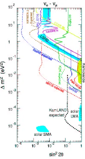
It is convenient to plot ∆m2 versus sin22θto determine the regions that a particular neutrino detector has access to, as shown in Figure 2.1. Several experiments have explored various regions and have not seen evidence of oscillations, thereby excluding these areas as solutions for neutrino oscillations. There are three theoretical solutions to the solar neutrino anomaly whose regions have yet to be explored. They are named the Large Mixing Angle (LMA), Small Mixing Angle (SMA), and Vacuum solutions. The LMA solution is the favored choice with the best fit solution at the time of KamLAND construction showing ∆m2 _{= 1}_.₈_×₁₀−5 _eV2 _{and sin}2₂_θ_{= 0}_._{76 [Bah98].}

KamLAND’s sensitivity to ∆m2_{can be estimated by calculating the upper and lower} limits for reactor neutrinos using Equation 2.13. For the upper limit, the shortest oscillation length Losc is 140 kilometers and the highest possible reactor neutrino energy is 8 MeV.

(22)

CHAPTER 2. THE KAMLAND EXPERIMENT 9 Seventh Meeting of the AAS High Energy Astrophysics Division 4

Figure 2.1: Neutrino exclusion plot as of March 1999. Allowed and excluded regions in the ∆m2₋_sin2₂_θ _{phase space for}_ν

e → νµ oscillation. The existing limits are compared with

(23)

range of ∆m2 _{that can isolate the LMA solution from the others. Thus, KamLAND is} expected to decisively confirm or refute the validity of this solution.

2.2 Detection of the Neutrino

KamLAND uses the charged current reaction of inverse beta decay to identify an electron anti-neutrino capture by the following reaction:

νe+p→n+e+. (2.14)

The positron energy is determined by the incident neutrino energy and the neutron - proton mass difference, Ee = Eν −∆Mn−p, where ∆Mn−p = 1.293 MeV. Therefore, the energy

threshold for this reaction is ∆Mn−p+me'1.8 MeV.

To calculate the interaction cross section for this reaction, the general differential cross section formula is used,

dσ

dΩ(a+b→c+d) = 1

4π2_~4|Mif| 2 p

2

f

υiυf

(2.15) where|Mif|is the matrix element between initial and final states involving integration over

spins and angles of the particles, pf is the center-of-mass system momentum of the final

state particles, and υi and υf are the relative velocities in the center-of-mass system of a

andb and ofc andd. For inverse beta decay, the matrix element is the sum over the Fermi and Gamow-Teller terms, given by

|Mif|2=G

¡

|MF|2+|MGT|2

¢

(2.16) where the Fermi constant G = 1.17×10−5 _GeV−2_, _|M

F|2 ' 1 for total lepton spins = 0

and |MGT|2'3 for total lepton spins = 1.

Using Equations 2.15 and 2.16 and integrating overdΩ, the lowest order cross section for inverse beta decay is given by

σ(νe+p→n+e+) =

G2 π

¡

|MF|2+|MGT|2

¢ p2 υiυf

(24)

Here, υi and υf are ' c and E is the positron energy in MeV [Per00]. For E ≈ 1 MeV,

this is a very small value, corresponding to a mean free path for the anti-neutrino of about 1020 _{cm, and can be compared to the low energy nucleon-nucleon scattering cross section} of 20×10−24 _cm2_.

The reaction in Equation 2.14 results in two signals, one prompt and one delayed that can be used to identify a neutrino event and eliminate many sources of background from consideration. The prompt signal occurs when the positron annihilates with an electron, producing two gamma rays with a total energy of 1.02 MeV plus the energy of the positron. The delayed signal occurs when the neutron thermalizes and is captured by another proton according to the reaction,

n+p→d+γ (2.18)

where the gamma has an energy of 2.2 MeV.

Because this delayed signal is essential for identifying a neutrino event, it is im-portant to know the mean neutron capture time. A simple model developed by Fujikawa [Fuj01] provides an estimate of this capture time in the KamLAND scintillator through the equation

1 τ =

ρNA

P

iniAi

v0 X

i

niσi(v0) (2.19)

whereτ is the capture time, ρ is the density of the scintillator, NA is Avogadro’s number,

ni and Ai are the relative number and atomic weight of isotopes i respectively, v0 is the thermal neutron velocity of 2200 meters per second, and σi is the neutron capture cross

section at v0 for isotope i.

Since KamLAND’s scintillator only contains hydrogen and carbon, Equation 2.19 can be simplified by usingrH, the hydrogen to carbon ratio,

1 τ =

ρNA

rHAH +AC

(25)

scintillator, their capture cross section, and the fraction of neutron captures. Only 1_{H and} 12_{C need to be used, since} _∼_{100% of the captures occurs on these isotopes. The density of} the scintillator is 0.78 g/cm3_{and the hydrogen to carbon ratio for the KamLAND scintillator} is 1.97. Inserting these numbers into Equation 2.20 results in an estimated mean neutron capture time of 205.2 µs [Fuj01].

Table 2.1: Isotopes in the KamLAND scintillator and selected properties. For each isotope, the capture cross section for neutrons with velocityv0 = 2200 m/s and the relative fraction of neutron captures are shown.

Capture Cross Section Fraction of Isotope

(barns per atom) Neutron Captures

1_H _0.3326 _99.45%

2_H _0.000519 ₂_×₁₀−7

12_C _0.00353 _0.55%

13_C _0.00137 ₂_×₁₀−5

The probability of eliminating false events is increased by introducing three cuts on possible neutrino events. Because the thermalization of neutrons can vary, a timing cut is established for the neutron capture. The captures must occur between 10 and 500 microseconds after the prompt signal occurs. The prompt gammas must have a combined energy in the range of 1.0 ≤E ≤8.0 MeV and the capture gamma energy must lie in the range between 1.8 and 2.7 MeV. Finally, the events must occur in close proximity to each other.

2.3 Detector Location and Components

(26)

KamLAND

(27)

The muon flux at the KamLAND site is compared to other underground experiments in Figure 2.3. KamLAND is buffered by over 1000 meters of rock or about 2700 meters water equivalent, which provides shielding from cosmic rays that have energies less than 1.3 TeV at the mountain surface and provides a well known muon attenuation factor of 105. The detector is comprised of two sections, called the Inner and the Outer Detectors and is detailed in Figure 2.4. The Inner Detector is comprised of two sections separated by a 13 m diameter spherical balloon made of 135 µm thick transparent nylon/ethylene vinyl alcohol copolymer composite film. Inside the balloon is approximately one kiloton of ultrapure liquid scintillator with a density of 0.78 g/cm3. It is comprised of 80% Dodecane and 20% Pseudocumene (1,2,4-Trimethylbenzene) for a hydrogen to carbon ratio of 1.97. In addition, 1.5 g/` of PPO (2,5-Diphenyloxazole) is added to act as a fluor. Between the balloon and the 18 m stainless steel shell of the Inner Detector is a buffer of dodecane and isoparaffin oils that provide shielding for the liquid scintillator.

The balloon is supported and kept in an approximate spherical shape by minimizing the differences in density between the scintillator and mineral oil and by a series of support ropes. Along the inside surface of the steel sphere in the mineral oil are 1325 seventeen inch and 554 twenty inch photomultiplier tubes (PMTs). These are arranged in a hexagonal lattice array and face in towards the balloon. The scintillator and mineral oil both produce directional ˘Cerenkov signals while the scintillator also produces large isotropic light signals from ionizing radiation.

(28)

Depth, meters water equivalent

(29)

TOP

BOTTOM SPHERE

BALLOON

17" PMT 20" PMT

TYVEK TYVEK

LOWER UPPER DOME

(30)

to eliminate dead zones. The Tyvek is placed behind the PMTs on the cavity’s surface as well as on the Inner Detector sphere.

(31)

Chapter 3

The Outer Detector

The success of large underground detectors like KamLAND heavily depends on the ability to understand and supress background. KamLAND’s background comes from natural radioactivity and cosmic ray muon-induced processes and the Outer Detector plays an important role in discriminating this background from true events. It actively tags and vetoes through-going cosmic ray muons in offline analysis by detecting their ˘Cerenkov radiation. It also acts as a passive shield by absorbing natural radiation and by moderating and absorbing spallation neutrons, which are produced when muons collide with nuclei in both the rock and the water.

3.1 Cerenkov Radiation

˘

Cerenkov radiation arises from the interaction of a charged particle traveling through a transparent medium, which in the KamLAND Outer Detector is a cosmic ray muon traveling through water. The electric field of the muon causes the nearby water molecules to behave like elementary dipoles by forcing the hydrogen atoms to rotate around the oxygen atom, such that they are further away (closer) to the negatively (positively) charged muon as seen in Figure 3.1. This causes the medium to become polarized about the point P.

(32)

CHAPTER 3. THE OUTER DETECTOR 19

As the muon continues along its track, the shape of the atoms around P returns to normal. Thus, each incremental region along the muon track will receive a very brief electromagnetic pulse in turn as the muon traverses the water. If the muon has a low velocity, the polarization field around the muon is symmetric in all directions. With such symmetry, there is zero resultant field at large distances and therefore, no radiation.

+ - +- + - + -- + + -- + + -+ - + - _{+ -} + - P - + + -+ - ₊ - _{+ -} + - - + +- - + +- - + P

Figure 3.1: The polarization of a dielectric that is set up when a charged particle passes nearby. The figure on the left is for a negatively charged particle traveling with a low velocity, while the figure on the right is for a high velocity particle.

If the muon is moving at a speed that is faster than that of light in the medium, then the picture is different. In this case, the polarization field loses its symmetry along the axis, resulting in a dipole field that is apparent at large distances from the muon track. This dipole field is momentarily set up by the muon in turn in each incremental region. Each region then radiates an electromagnetic wavelet of light over a band of frequencies.

(33)

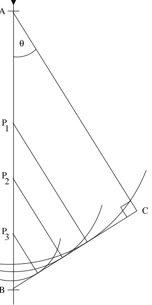
an angle, θ, with respect to the muon track. Although Figure 3.2 has been drawn in two dimensions, the ˘Cerenkov radiation is produced in complete symmetry about the axis of travel and propagates along the surface of a cone with the angle θ.

B

Α

θ

C P

3 P

1

P 2

Figure 3.2: The coherence of the radiated wavelets from arbitrary points, such as P1, P2, and P3, produce a unified wavefront along BC at a specific angle, θ. This angle depends upon the medium through which the charged particle is traveling.

(34)

given by

cosθ= 1

nβ. (3.1)

From this equation, it can be seen that for a particle whose relativistic velocity approaches c, the maximum angle of emission is given by θmax = cos−1(1/n). The radiation that is

produced has wavelengths mainly in the visible and near-visible regions of the spectrum, as long asn >1. Since the medium of the Outer Detector is water, this results inθmax = 41.2◦

with a wavelength in the blue region.

There are three more conditions that must be met in order to achieve coherence. The velocity of the particle must be above a minimum, set by βmin = (1/n), in order to

produce radiation. In order to avoid diffraction, the path length of the particle through the medium must be large compared to the wavelength of the emitted radiation. Finally, the velocity of the particle through the medium must remain constant [Jel58].

3.2 Neutron Spallation

Spallation is a two stage process on the nuclear level. In the first stage, the incident particle collides with nucleons inside the nucleus, which causes a series of intranuclear cascades. The end result is the ejection of various types of nucleons from the nucleus, which is now left in an excited state. As the imparted energy from the original collision is distributed over the nucleus, low energy particles evaporate from the surface as part of the second stage. Finally, the remaining excitation energy is dissipated by the emission of gamma rays.

(35)

(LVD) at Gran Sasso [Agl99] and from various proton decay experiments [Kha83]. In addition, a Monte Carlo simulation [Wan01] is also shown.

1.E-02 1.E-01 1.E+00 1.E+01 1.E+02 1.E+03

0 0.2 0.4 0.6 0.8 1 1.2 1.4 1.6 1.8 2

Neutron Energy (GeV)

Arbitrary Units _LVD

Khalchukov

Wang et al.

Figure 3.3: A comparison of two experimentally derived models (Large Volume Detector at Gran Sasso (LVD) [Agl99] and various proton decay experiments [Kha83]) and a Monte Carlo derived spectrum (Wang et al. [Wan01]) for spallation neutrons. Each model is normalized to unity at 400 MeV.

3.3 Relevance to KamLAND

The Outer Detector detects and tags through-going cosmic ray muons by their tell-tale ˘Cerenkov radiation. For those muons that also pass through the Inner Detector, the Outer Detector acts as an anti-coincidence veto, thereby removing the muons from consideration.

(36)

particles. The ionized particles are immediately slowed and neutralized and the low energy neutrons are absorbed by the water. Due to the very short distances needed to attenuate these types of particles in the Outer Detector, this background is negligible.

However, the high energy neutrons produced by spallation are the dominant source of background, one that can have a major effect on the results of KamLAND. If such a neutron scatters off protons in the Inner Detector, the proton recoils could mimic a positron signal. If the neutron is then captured by another proton and the three data cuts for a neutrino event are satisfied, a fake neutrino event will be recorded. Figure 3.4 shows the Feynman diagrams for real and fake events.

p

γ

d n

p

n

p n

p

γ

d n

ν− W+

e+ n p

Figure 3.4: Feynman diagrams of real and fake events. The top figure shows the process for a real neutrino event: the inverse beta decay of a proton followed by the neutron capture. The bottom figure represents the fake event which is characterized by the proton-neutron scattering process, which can occur several times, followed by the neutron capture. Time increases from left to right.

(37)

spatial and time cuts around the muon path. For this reason, the muon detection efficiency by the Outer Detector must be as high as possible to identify and eliminate neutrons produced by through-going muons.

(38)

Chapter 4

Photomultiplier Tube Testing

At the conclusion of the Kamiokande neutrino experiment in 1995 and prior to the formation of the KamLAND collaboration, approximately 1000 twenty inch PMTs were removed from the experiment site and placed into a nearby storage facility at the Kamioka mine site. During the summer of 1999, a simple testing facility was set up at the storage site to determine the state of these PMTs. They were connected to 1500 volts and the dark noise signal was observed. PMTs denoted ‘good’ had dark pulses less than 10 mV. Good PMTs also had a dark current of approximately 0.55 mA. Dead PMTs were observed to have dark currents of 10 mA or greater. This preliminary testing produced 842 PMTs that were considered good and they were shipped to Sendai, Japan for further testing. An additional 50 untested PMTs were already located in Sendai, giving a total of 892 from which to select the Outer Detector PMTs.

The PMTs were comprised of four different types, with each sucessive model repre-senting an improvement in design. Three types were used in the Kamiokande experiment, labeled ‘A’, ‘B’, and ‘C’. The first two types were developed specifically for that experiment while the ‘C’ type PMTs, which were developed for the upcoming Super-K experiment, were used towards the end of the Kamiokande experiment. The fourth type, denoted ‘SK’, was used only for testing purposes during the design phase of Super-K.

(39)

CHAPTER 4. PHOTOMULTIPLIER TUBE TESTING 26

The main difference between the four types is that the ‘A’ and ‘B’ type PMTs have a 13 stage dynode assembly while types ‘C’ and ‘SK’ have an 11 stage dynode assembly. Types ‘C’ and ‘SK’ also show a clear single photoelectron peak response and have an improved timing response. However, since muon events typically produce more than one photoelectron per PMT and because of the presence of Tyvek in the Outer Detector, these differences in PMT technology do not affect the ability of the Outer Detector to act as a veto for the Inner Detector.

4.1 Test Bench Setup

Due to coverage requirements for the Inner Detector, 600 PMTs (mostly ‘B’ types with some ‘A’ types) were taken from the stock for use in the Inner Detector. In order to supply the best PMTs for the Outer Detector, a thorough analysis of the remaining 290 PMTs (containing all four types) was performed to determine their worthiness for installation. This analysis consisted of first verifying the integrity of a PMT by examining it for evidence of broken components and a loss of vacuum. If it was intact and the resistance in the signal and high voltage cables measured 50 Ω and greater than 5 MΩ respectively, it was deemed fit for use.

(40)

Gate

Laser

TTL−>NIM

Laser Monitor

Discriminator

Monitor 1

Monitor 2

Gate & Delay Generator

Delay Delay Delay Scalar Delay Gate & Delay

Generator Pulser

PMT x 6 Attenuator Amplifier

Attenuator Amplifier

Amplifier Attenuator

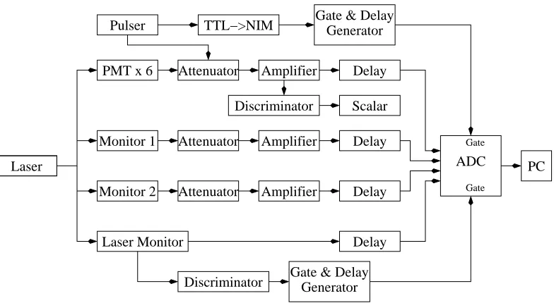
ADC _PC

Figure 4.1: Block diagram of electronics for high voltage testing. The pulser is used for the charge/channel calibration while the laser is used for the high voltage testing.

(41)

Physics Analysis Workshop (PAW) [App95] was used to plot the histograms for the tested PMTs and to obtain Gaussian fits to the peaks. These peak values were recorded on paper and the histogram data were saved to file. When the testing of six PMTs was finished, all associated files are deemed a ‘Set’ and were stored for later analysis.

Figure 4.2 shows a typical laser response spectrum for a PMT (Serial #0245, a type ‘C’ PMT). The channel number of the peak is derived from fitting procedures using PAW for all six PMTs under test and for the three monitor peaks. The program fits the peaks to a Gaussian shape using a range of channel numbers determined by the width at 40% of the height.

Figure 4.2: Fitted histogram for PMT #0245. Laser response spectrum for type ‘C’ PMT, serial #0245, during Set 25, measurement 1. The channel number of the peak,Cp, is derived

(42)

4.2 Gain and Gain Response Function for Photomultipliers

For an n-stage photomultiplier, the response function of the gain, G, with respect to the high voltage,V, is given by

G=δn=κVα (4.1)

whereδ is the average secondary electron emission ratio andκand αare empirically deter-mined constants. The constantα is given by

α=nαo (4.2)

whereαois a coefficient determined by the dynode material and geometric structure [Ham00].

This form of the response is valid in the operating region of the PMT. The gain for a PMT at a specific voltage can be calculated by

G= Qp

eN (4.3)

whereQp is the amount of charge collected by the PMTs in Coulombs,eis the charge per

photoelectron (1.6×10−19_C/_e−_{), and} _N _{is the number of photoelectrons produced by the}

photocathode in response to the incident laser photons. The intensity of the laser signal can be reduced until only a single photoelectron is being produced (N = 1).

The charge,Qp, is given by

Qp =

Cp−Co

m (4.4)

where Cp is the channel number of the laser pulse peak, Co is the constant channel offset

due to the electronics DC level, and m is the conversion factor from channel number to charge. Cp values are measured for several voltages, spanning a range of 500 V for each

PMT, according to the voltage testing procedure.

Values of Co and m are determined by a calibration process whereby square wave

(43)

By measuring the voltage height, V, and the time width, t, of the pulse and knowing the impedance, Z (50 Ω), of the circuitry, the value of the input charge was obtained from

Q= V t

Z (4.5)

Typical numbers were V = 860 mV and t = 40 ns. This calibration was performed with several different voltages at the three attenuations (0, 40, and 52 dB) for all six bins’ electronics.

A fitted calibration plot is shown in Figure 4.3. A linear fit program [Fas88] was used to calculate the conversion factor, m (pC/ch), and the offset, Co (ch). Using these

data, all the peaks from the voltage test were converted to an amount of charge.

The position test was used to determine whether the angle of incidence of the laser affects the number of photons seen by the PMT. One PMT of each type (A - serial #4014, B - #0022, C - #0265) was placed in a bin in a normal manner and a peak channel measurement taken. On subsequent runs, the PMT was tilted at an angle, Θ, rotated an angle, Φ, or a combination of these, as seen in Table 4.1.

Table 4.1: Position of a PMT during position testing

Run # Θ Φ

1 0 0

2 0 90

3 20 90

4 20 180

(44)

CHAPTER

4.

PHOTOMUL

TIPLIER

TUBE

TESTING

31

Charge per Channel Calibration at 52dB (Bin1)

-500 0 500 1000 1500 2000 2500 3000

0 200 400 600 800 1000 1200 1400 1600

Channel #

Charge (pC)

Charge (pC) Linear Fit

Figure 4.3: Charge per channel calibration for Bin 1 at 52 dB. Varying amounts of chargeQwere input into the ADC circuitry. The data were fit to a straight line to yield the slopem(pC/ch) and the channel offsetCo for each bin at each attenuation. With

this information, the peaks from the voltage test were converted into the amount of charge,Qp. The error in the amount of input

(45)

CHAPTER

4.

PHOTOMUL

TIPLIER

TUBE

TESTING

32

Gain vs. Changing Positions

0.40 0.50 0.60 0.70 0.80 0.90

0 1 2 3 4

Measurement #

Gain (e7)

#0265 #0022 #4014

(46)

4.3 Analysis of the Single Photoelectron Peaks

For the purpose of the gain calculation in Equation 4.3, the number of converted photoelectrons,N, induced by the laser illumination must be known. Ideally, this value is determined by a comparison with the single photoelectron (SPE) peak. However, of the four types of PMTs used for the Outer Detector, only the ‘C’ and ‘SK’ types are capable of seeing a single photoelectron peak. The 17” Inner Detector PMTs can also detect the SPE peak. A 20” ‘C’ PMT serial #0245 at 2108 V and a 17” PMT serial #0021 at 2262 V were used to determine the responses. SPE spectra for the type ‘C’ and the 17” PMTs are shown in Figure 4.5.

The Inner Detector electronics setup used the laser pulse to gate the ADC. As a result, the noise spectrum cannot be readily obtained by turning off the laser. Instead, different combinations of laser filters were used to reduce the intensity until the number of photoelectrons produced by the photocathode decreased to one. This was verified when the channel number of the SPE peak stopped decreasing (meaning that the minimum amount of charge had been collected) and the number of counts in the peak for a given collection time started decreasing (indicating that not every laser pulse was producing a photoelectron).

The location of the SPE peak was converted into an equivalent amount of charge using the results of the charge/channel calibration. Equation 4.4 yielded the result of 0.88±0.08 pC for PMT #0245 and 1.37±0.07 pC for PMT #0021. It is necessary to compare these results with the voltage testing data obtained for these PMTs so that the number of photoelectrons, N, induced by the laser illumination during the voltage test is known. These two PMTs were tested together in Set 25, with measurement 1 (Set25m1) having the same voltage as in the SPE test. Using the equation,

1 N =

Q(SPE)

Q(Laser) (4.6)

(47)

(48)

laser illuminates both tested PMTs equally and that the photocathode responses are the same.

Since the noise in the type ‘A’ and ‘B’ PMTs is too high to show a single photo-electron response, they cannot be calibrated in the same way. Instead, it must be assumed that the photocathode responses of all PMTs are the same and that this same laser il-lumination would have yielded an average of N = 375 in all of the PMTs. In practice, the amount of laser illumination does change over time and affects the actual number of photoelectrons detected. This was taken into account by normalizing to the monitor:

N = 375

ρ (4.7)

whereρ is defined by

ρ= monitor value of Set25m1

monitor value of data point (4.8)

In this way, the differences in illumination for each measurement set were accounted for.

4.4 Photomultiplier Tube Testing Results

Using Equations 4.3, 4.4, and 4.7, the gain of a PMT can be calculated for a par-ticular high voltage. A typical set of results is shown in Figure 4.6. The data were fitted to Equation 4.1 and values of κ and α were determined for each PMT. Typical numbers are 10−20 _{to 10}−25 _{and 7.5 to 10.4 respectively. Using Equation 4.2, the data was compared to} the expected value for αo. For 13 dynode stage systems (types ‘A’ and ‘B’), the average

value of αo = 0.71. For the 11 dynode stage systems (types ‘C’ and ‘SK’), the average

value ofαo= 0.75. These results are in agreement with the Hamamatsu predicted range of

0.7< αo <0.8 [Ham00].

The voltage required for a specific gain was calculated by V =

µ G

κ ¶_α1

(49)

CHAPTER

4.

PHOTOMUL

TIPLIER

TUBE

TESTING

36

Gain and Gain Response Function vs. High Voltage for PMT #0245

0 4000000 8000000 12000000 16000000 20000000 24000000

1950 2050 2150 2250 2350 2450 2550

High Voltage

Gain

Gain Values Response Fit

Figure 4.6: Gain versus high voltage plot for PMT #0245 with fit. The gains for six measured voltages are plotted versus voltage, where the gains have an error of 3.8%. These points are then fitted to Equation 4.1. For type ‘C’ PMT (Serial #0245),

(50)

change in high voltage required for a±5% change in the gain, the Hamamatsu voltage value forG= 0.6×107_{, and the PMT dark current rate. In addition, other relevant information} is presented in Appendix B: PMT location, PMT voltage cable labels, and PMT signal cable labels.

The location code for a PMT is of the form R-A-XXX. The first symbol, R, repre-sents the region where the PMT has been installed. The top region is denoted by ‘T’, the side region by ‘S’, and the bottom region by ‘B’. The second symbol,A, labels the PMT row within the region. For both the top and bottom regions, the rows are numbered sequentially starting with the outermost ring of PMTs and proceeding inwards. For the side region, the rows are numbered starting at the top and increasing towards the bottom. The final set of symbols,XXX represents the angle, Φ, of placement. A PMT with tag T-1-207is located in the top region, in the outermost row, at Φ = 207◦_{. A schematic of the PMT locations}

can be seen in Figures 4.7 and 4.8.

Figure 4.9 shows the difference in high voltage values between the measured values and those of Hamamatsu for G = 0.6×107_{. In general, the tested values were slightly} higher, typically of order 20 - 50 volts. This is most likely due to the expected deterioration of the dynodes over time. Large ∆V were taken as evidence of a potential problem and the PMTs were accordingly flagged.

(51)

B−4−XXX

T−3−XXX

S−2−XXX

ROW 2

ROW 6 ROW 5 ROW 4 ROW 3 ROW 1

BOTTOM SIDE TOP

ROW 1 ROW 3 ROW 3 ROW 1

ROW 2 ROW 4 ROW 4 ROW 2

ROW 3

ROW 2 ROW 2

ROW 3

ROW 1 ROW 1

(52)

N

9

27

81

135

45

63

117

99

(53)

CHAPTER

4.

PHOTOMUL

TIPLIER

TUBE

TESTING

40

Fitted - Hamamatsu HV Values

-750 -650 -550 -450 -350 -250 -150 -50 50 150 250 350 450 550 650

Serial #

Difference in Voltage

December Data Double Tested Dec. Double Tested June June Data

(54)

CHAPTER

4.

PHOTOMUL

TIPLIER

TUBE

TESTING

41

Adjusted Fitted - Hamamatsu HV Values

-200 -150 -100 -50 0 50 100 150 200 250

Serial #

Difference in Voltage

December Data Adjusted June Data

(55)

After all the calculations and fitting had been done, there were three additional cases where a PMT was rejected as being unfit for use in KamLAND. Due to factory specified voltage limits, PMTs that had a projected operational voltage greater than 2550 V were rejected. Secondly, PMTs were rejected if the gain response function was irregular. Finally, the dark current rate must be below 50 kHz. In addition, the testing region that includes the expected operating voltage for a gain of 1.0×107 was checked. For four PMTs (Serial #0053, #0272, #0757, and #3938), this voltage value lies beyond the testing range. The high voltage that corresponds to G = 1.0×107 for these four PMTs was determined by extrapolating the gain response function. It should be noted that there is some level of uncertainty in projecting a high voltage since the gain response function will eventually saturate and there will be sensitivity to changes in the local magnetic field.

Of the 278 twenty inch PMTs tested, there were a total of 19 that were rejected (see Table 4.2). Thus, there are 259 PMTs available for use in KamLAND that have a good gain response curve, moderate operational voltage, and low noise. From these 259 PMTs, 225 were selected for installation. The number of each type is as follows: 95 type ‘A’, 60 type ‘B’, 51 type ‘C’, 15 type ‘SK’, and 7 of unspecified type.

Table 4.2: Rejected photomultiplier tubes

Serial # of PMTs Reason for Rejection

3194, 3677 Unable to hold high voltage

3048 Irregular gain response function

0005, 0022, 0072, 0134, 0715, 4014 Dark current rate above threshold − − − Operational high voltage above threshold 0243, 0244, 0250, 0299, 0357, Failed after installation

(56)

Chapter 5

Construction of the Outer Detector

The construction process started in October 1999 and went through the closing of the Outer Detector hatch in April 2001. Several small projects were needed to solve various problems and meet design parameters as the Outer Detector was being built. The projects included refurbishing the PMTs, obtaining cable, developing a splicing design, and installing the PMTs and Tyvek.

5.1 Refurbishment of the PMTs during Testing

During the testing phase in Sendai, several actions were performed to refurbish the PMTs for eventual re-use. It was noted that many PMTs had dust, grime, grease and remnants of epoxy on the glass in the photocathode region. The PMTs were given a preliminary cleaning by the testers and then a final cleaning by members of the Honda-Seiki company.

Waterproofing the PMT bases was also performed during this time since it was known that approximately 20% of Kamiokande’s dead PMTs failed due to water leakage. This leakage is thought to have occured whenever Kamiokande was emptied and refilled, thereby setting up thermal gradients that caused the original sealant to crack. Although KamLAND should experience very few filling cycles, the condition of the original sealant

(57)

CHAPTER 5. CONSTRUCTION OF THE OUTER DETECTOR 44

and the age of the PMTs was a concern. Using a soft urethane based two part epoxy, the Pyrex/PVC interface at the base was coated and allowed to dry.

The last action taken during the testing phase was to remove the excess lengths of signal and high voltage cables for every PMT. During the breakdown of the Kamiokande experiment, the cables were cut for easy removal of the PMTs and they were left with approximately three feet of cable still attached at the base. It was assumed that during the subsequent handling and storage, these cables were likely to have suffered damage. Therefore, to minimize the possibility of failure in a water environment, both the signal and high voltage cables were cut to a length of approximately one foot to allow for cable splicing.

5.2 Cable Requirements and Splicing Design

The next step in preparing the PMTs for installation was to determine the cable routing and lengths for the cables and to decide how to splice the new cable with the original cables. Although the old signal cables were R-174 and the high voltage cables were RG-58, it was deemed best to use RG-58 cable for the signal and RG-59 for the high voltage, since these are standards today. The ‘RG’ denomination represents quarter inch coaxial cable with a resistance of 50 ohms. For added protection against water leakage, it was decided to buy blocked cable, which impedes the flow of water in the cable if there is a hole or cut in the outer jacket insulation. Blocked cable is made during manufacturing by forcing a liquid under the cable jacket which solidifies on the braid of the wire. This type of cable was used in both the Super-Kamiokande and the Sudbury Neutrino Observatory experiments. It was also necessary for the cables to have a polyethylene jacket, since this material does not promote algae growth when placed in a pure water environment.

(58)

the TUNL design would use standard high quality BNC connectors to splice the two sets of cables together. Although blocked cable is slightly thicker due to the extra material, normal BNC connectors can still be attached sucessfully. The BNC connectors are of the two-part crimp style, which is more reliable for electrical connections compared to the one-part crimp or the solder type of connectors. By crimping the ends with the proper tools, there is no reliance on soldering, which can be inconsistent and subject to failure as a result of mechanical or temperature stresses. In addition, a small amount of rubber silicon sealant, RTV-112, is placed into the BNC conector between the outer crimp jacket and the grounded cable shield to provide an additional water block between the outside and the inner connector.

For the high voltage splice, a standard female connector was crimped onto the PMT cable. The water blocked cable had a standard male connector placed on one end for the splice and an SHV connector crimped on the other end for connection to the high voltage power supply.

Because of the need for the inclusion of a 50 Ω terminator in the signal cable, the TUNL design incorporated a unique but simple and cost effective way of implementing this feature. Instead of using internal termination female-female barrels (approximate cost of $26 each), simple female-male-female ‘T’ connectors were modified (cost <$3/connector) by cutting off the male branch and leaving a straight barrel. A small ‘board type’ 1₈ watt 50 Ω resistor was soldered in place across the exposed pin and epoxy was used to enclose the resistor and seal the cut branch. See Figure 5.1 for a diagram of the modified connector. The ends of the signal cables all have a standard male connector.

(59)

CHAPTER 5. CONSTRUCTION OF THE OUTER DETECTOR 46 TOP VIEW TEFLON DIELECTRIC CHIP SOLDERED

TO PIN AND CASE 50 OHM RESISTOR

EPOXY SIDE VIEW

Figure 5.1: A standard ‘T’ connector was modified to produce a 50 Ω terminated straight barrel.

The splicing method was tested at TUNL using both high pressure air and high pressure water. The BNC plug ends were crimped with RTV-112 sealant onto the ends of regular (not water blocked or treated) RG-58 cable. A few cuts were sliced into the outer jacket of the cable in one area. A Swagelock ‘T’ and fittings were placed around these cuts for the attachment of an air hose or water hose. Approximately 60 psi of Argon gas was forced into the cable through the cuts in the outer jacket. The splice and ‘T’ fittings were immersed in water to look for escaping gas bubbles, which would signify a leak. However, there were no leaks around the Swagelock fittings nor from the BNC ends. The test was then continued for a period of three weeks with 40 psi of water without any leaks. Since these pressures were far greater than what is expected at KamLAND, the TUNL splicing method was proven robust.

(60)

was used. Because of this complication, the splicing was done at Sendai during the assembly of the PMTs with frames and shielding. To install the small board, the cable was cut about two feet from the PMT. The outer jacket was pulled back so the high voltage and signal cables could be stripped and then soldered onto the board along with the accompanying water blocked cables. Shrink wrap was heated up to the board, at which point RTV-112 was injected into the wrap around the board. Because two cables come out from the other side of the board, the shrink wrap was slit lengthwise a few inches to allow the wrap to contract around both cables and seal to itself. Heating of this side of the shrink wrap locked in the RTV and provided another layer of protection against water leakage.

5.3 Cable Routing Scheme

It is desirable to have the Outer Detector and Inner Detector PMT signals arrive at the electronics at the same time. Due to velocity matching of the two sets of cables, the Outer Detector signal cables had to be 42 m in length while the Inner Detector cables were 40 m. Since these lengths allowed the cables to just reach the dome area, additional extension cables were needed to reach the electronics hut (e-hut) and connect to the electronics. There were no restrictions on the high voltage cable lengths other than the requirement that they reach the high voltage distributors in the hallway outside the dome entrance.

The cables make their way out of the detector cavity and into the dome by way of two cable holes at 130◦ _{and 298}◦_{. Figure 5.2 shows the locations of the cable holes, the}

e-hut, the high voltage distributors, and the cable routes of the signal and high voltage cables across the dome.

5.3.1 Signal Cables

(61)

CHAPTER 5. CONSTR UCTION OF THE OUTER DETECTOR 48 7 8 9 11 12 10 3 2 1 5 4 6 180 N 0 HV Distributors Outer Detector Cable Trays Inner Detector Cable Trays o o Entrance Dome Rock Wall E-hut

(62)

straight to the nearest cable hole, as seen in Figure 5.3. Supporting frames and beams were used to secure the cables and keep them above the photocathodes and behind the Tyvek to prevent shadowing.

hole 298 cableo

cable hole130

o

0o

pmt

cables

16 meters N

Figure 5.3: Cable routing for top PMTs. Cables travel along each radial beam to the wall, then are routed directly to the nearest cable hole.

(63)

The PMTs on the bottom section were the limiting factor in meeting the length requirement since they are the farthest from the cable holes. The routing scheme used the PMT support beams on the floor to secure the cables and keep them below the photo-cathode. These beams run radially out to the wall, where the cables were then routed around the circumference of the detector cavity to the side PMT supports that are below the cable holes. Each group of cables were secured to this support structure up through the cable hole into the dome. Figure 5.4 shows the routing pattern for each bottom PMT.

Up to 298o hole

130 hole Up to

o

0o

16 meters

pmt

cables

N

(64)

Signal cables that pass through the 298◦ _{hole traveled along the circumference of}

the dome towards the e-hut as shown in Figure 5.2. Cables from the 130◦ _{hole entered the}

dome directly behind the e-hut where they meet with the other signal cables at the cable entrance of the e-hut.

5.3.2 High Voltage Cables

The high voltage cables followed the same routing as the signal cables for each of the three regions to the dome from the Outer Detector cavity. The high voltage cables entering the dome from the 130◦ _{hole enter a cable tray and travel around the circumference to a}

position near the entrance to the dome at 244◦_{. Cables routed to the 298}◦ _{hole also enter a}

cable tray, travel along the circumference of the room to approximately the 270◦ _position,

where they were then routed up and over the dome entrance and then back down to the floor at the 244◦ _{position. At this point all high voltage cables were in one group and}

pass through the wall next to the entrance. The high voltage power supply for the Outer Detector is located in the farthest power supply bin from the dome entrance. Therefore, the cables traveled up and over the supply bins and then back down to the individual plugs in the rear of the Outer Detector bin.

To keep the amount of cable to a minimum, cable lengths were split into three groups: bottom PMTs, lower hemisphere PMTs, and the top and upper hemisphere PMTs. Calculations of the lengths based on the aforementioned routing gave the bottom PMTs a maximum length of 70 m, while the lower hemisphere PMTs and the upper and top PMTs had lengths of 61 and 51 m respectively.

5.4 Cable Production

(65)

to prevent abrasions on the outer jacket, the cable was unrolled from the spools, measured to the various lengths required, and then cut by TUNL personnel. Each cable was then coiled and placed inside an individual plastic bag for further protection.

Next, the two appropriate BNC connectors were crimped onto the cable ends. The quality of the crimp was tested by using a voltmeter to confirm a closed circuit from pin-to-pin and from ground-to-ground and an open circuit from pin-to-ground. In addition, since it would not be known which cable would be connected to which PMT until splicing, small character labels were placed on each end of the coils. In this manner, the correct PMTs could be connected to the right channels in the electronics crate and high voltage power supply. Finally, the bagged cables were packed into crates and shipped directly to the Kamioka mine site in September 2000. Approximately 200 person-hours were used for this process of cutting and crimping.

5.5 PMT Frames and Shielding

During June 2000 in Sendai, those PMTs that were determined to be reliable and in good standing from the gain testing stage underwent further refurbishment. For the ‘A’, ‘B’, and ‘C’ type PMTs, heat shrink tubing was applied to the existing cables before the BNC connectors were crimped on. The crimps were tested by using a voltmeter and measuring 50 Ω on the signal cable and 5 MΩ on the high voltage cable. For the 13 ‘SK’ type PMTs, the actual splice was performed according to the procedure described in Section 5.2. Because these PMTs were newer and had a better seal around the base, it was desired to use these PMTs near the bottom where the water pressure would be greatest. Therefore, cables of 61 m were spliced to six PMTs that were to be placed on the lowest side level and cables of 70 m were spliced to the rest that would be placed on the bottom.

(66)

attached to a metal frame, which would be used to attach the PMT to the support structure in the Outer Detector. Labels which listed the PMT serial number were attached to the frame to aid in identification after installation. The completely refurbished PMTs were then placed in bags and secured in boxes. Approximately 14 person-weeks of TUNL labor was used to complete these tasks. The PMTs were then shipped from Sendai to the mine site in late July 2000.

5.6 Installation of PMTs and Tyvek

In December 2000, the framed PMTs were unpacked in the mine and epoxy was applied around the base of the PMTs at the boundary of the PVC and the old epoxy to further waterproof them. The 170 PMTs for the top and side levels of the Outer Detec-tor were then provided to workers of the Mitsui Shipbuilding Corporation for installation because installation of these PMTs required maneuvering the framed PMTs on scaffolding and through tight spaces. Japanese insurance regulations did not allow for anyone other than the Mitsui workers to carry the PMTs around on the scaffolding. Bottom level PMTs were set aside until after the scaffolding was removed from the cavity and the bottom region cleaned.

After the installation of the side and top level PMTs, the high voltage and signal cables were strung and secured according to the routing schemes and connected to the PMTs’ cables. Because the scaffolding would be removed before the bottom PMTs would be tested, extra cables were strung in the event that they may be needed as replacements at a later date. The PMT serial number, its location within the Outer Detector, and the associated labels for the high voltage and signal cables were recorded. The location code used to describe the PMT position can be found in Section 4.4.

(67)

was checked as well as verifying that the cables being measured were actually connected to the PMT being tested. If these checks passed, then the resistance of the PMT-side cables from the PMT were tested. If the PMT did not pass this test, it was determined to be dead and was replaced. If the resistance was satisfactory across the PMT-side cables, then the resistance of the PMT was measured across the whole length of the water blocked cables. At this point, it could be determined if a strung cable was bad and it was subsequently replaced.

Three PMTs were determined to be inoperable from the top and sides during the post-intallation testing and they were replaced. In addition, three high voltage cables needed to be replaced. Retesting was performed on these PMTs until all installed PMTs were shown to be operable.

With all the PMTs testing satisfactorily, the heat shrink tubing was then heated around the cable splice with a heat gun to ensure a watertight seal. Cables for the bottom PMTs were strung and secured down to the last level of side PMTs. There they were temporarily stored in plastic bags and hung off of the structure to keep them from being damaged during the removal of the scaffolding and the subsequent cleaning of the bottom region.

The KamLAND Outer Detector

Biography

Personal

Education

Academic Positions

Memberships

Publications

Acknowledgements

Contents

List of Figures

List of Tables

Chapter 1

Introduction

Chapter 2

The KamLAND Experiment

2.1

Theory of Neutrino Oscillations

2.2

Detection of the Neutrino

2.3

Detector Location and Components

Depth, meters water equivalent

Chapter 3

The Outer Detector

3.1

Cerenkov Radiation

˘

3.2

Neutron Spallation

3.3

Relevance to KamLAND

Chapter 4

Photomultiplier Tube Testing

4.1

Test Bench Setup

4.2

Gain and Gain Response Function for Photomultipliers

4.3

Analysis of the Single Photoelectron Peaks

4.4

Photomultiplier Tube Testing Results

B−4−XXX

T−3−XXX

S−2−XXX

Chapter 5

Construction of the Outer Detector

5.1

Refurbishment of the PMTs during Testing

5.2

Cable Requirements and Splicing Design

5.3

Cable Routing Scheme

5.4

Cable Production

5.5

PMT Frames and Shielding

5.6

Installation of PMTs and Tyvek