Implementation and Sensitivity Analysis of a Task-Capability Interface Model for Automobile Driver Safety.

(1)

ABSTRACT

LYNCH, CAMERON EDWARD. Implementation and Sensitivity Analysis of a Task-Capability Interface Model for Automobile Driver Safety. (Under the direction of Dr. Mo-Yuen Chow.)

As technologies like GPS navigation systems, smart phones, and advanced on-board

computers increase their presence in the automotive world, it is natural to want to utilize

these resources to aid in improving automobile driver safety. Many current methods for

modeling drivers and driver safety are computationally expensive or inappropriate for

real-time use. To solve the problems of complexity, we wish to create a model that is

simple, understandable, and heuristically sound. In this study we design and implement

a version of the Task-Capability Interface(TCI) Model to accomplish these stated goals.

The TCI designed in this study uses three inputs, sleepiness, rainfall, and relative speed,

to determine task capability, task demand, and uses the difference to signal driver safety.

To compensate for the inexact nature of the problem, the TCI was implemented as a fuzzy

logic rules-based system. Further insight into the models behavior is obtained through

local sensitivity analysis with respect to sixteen of the membership function parameters.

This local sensitivity analysis reveals that four of the sixteen parameters have a significant

impact on the models behavior and should receive extra consideration when tuning the

model. Additionally, we consider the set of inputs that cause capability and demand to

be close in value. We find that these “borderline” inputs occupy a significant portion of

(2)

c

(3)

Implementation and Sensitivity Analysis of a Task-Capability Interface Model for Automobile Driver Safety

by

Cameron Edward Lynch

A thesis submitted to the Graduate Faculty of North Carolina State University

in partial fulfillment of the requirements for the Degree of

Master of Science

Electrical Engineering

Raleigh, North Carolina

2011

APPROVED BY:

Dr. Cranos Williams Dr. Ralph Smith

(4)

DEDICATION

This work is dedicated to my parents Eddie and Rhonda Lynch, as well as my fianc´e

(5)

BIOGRAPHY

Cameron Lynch was born in Wilmington, North Carolina on May 27th, 1985. He

re-ceived his Bachelors of Science in Electrical Engineering, Computer Engineering, and

Applied Mathematics at North Carolina State University in May of 2008. After entering

the Graduate School at North Carolina State University in the Fall of 2008 in pursuit

of a Master’s of Science in Electrical Engineering, he joined the Advanced Diagnosis,

Automation and Control Laboratory (ADAC Lab) under the direction of Dr. Mo-Yuen

Chow in the Fall of 2009 and has been working there ever since. Cameron’s research

interests include control systems, modeling, digital signal processing, and embedded

sys-tems. The defense of this thesis will complete the requirements to receive a Master’s of

(6)

ACKNOWLEDGEMENTS

I would like to take this time to thank my advisor, Dr. Mo-Yuen Chow for his time and

commitment to me throughout this process of conceiving and finishing my thesis project.

His knowledge and guidance proved to valuable resources and this work would not have

been possible without him. Additionally, I would like to thank the other members of my

committee, Dr. Ralph Smith and Dr. Cranos Williams, both of whom have impacted

me greatly as a student. My time here at North Carolina State University has been very

special to me, not only from an academic standpoint, but also on a personal level. I know

I will never forget my experiences here and I will try to stay engaged with the university

community.

This research was supported under NSF-ECS-0823952 Impaired Driver Electronic

Assis-tant (IDEA) project and DOT Massive Sensor Based Congestion Management System

(7)

LIST OF TABLES

Table 3.1 Capability Input Membership Function Parameters . . . 17

Table 3.2 Capability Output Membership Function Parameters . . . 18

Table 3.3 Demand Rainfall Membership Function Parameters . . . 21

Table 3.4 Demand Speed Membership Function Parameters . . . 22

Table 3.5 Demand Output Membership Function Parameters . . . 23

Table 4.1 Sleepiness Membership Function Parameter Sensitivity . . . 36

Table 4.2 Capability Output Membership Function Parameter Sensitivity . . 40

Table 4.3 Rainfall Membership Function Parameter Sensitivity . . . 46

Table 4.4 Speed Membership Function Parameter Sensitivity . . . 50

Table 4.5 Demand Output Membership Function Parameter Sensitivity . . . 54

Table 5.1 SL1 Analysis Results . . . 57

Table 5.5 C1 Analysis Results . . . 60

Table 5.8 R1 Analysis Results . . . 63

Table 5.11 S1 Analysis Results . . . 65

Table 5.14 D1 Analysis Results . . . 67

Table 5.15 D2 Analysis Results . . . 68

(10)

LIST OF FIGURES

Figure 2.1 An example of a membership function u with input x. . . 5

Figure 3.1 Task-capability interface model. . . 13

Figure 3.2 Task difficulty homeostasis. . . 14

Figure 3.3 Capability Input Membership Functions. . . 17

Figure 3.4 Capability Output Membership Functions. . . 18

Figure 3.5 Capability Model Input-Output Mapping . . . 19

Figure 3.6 Demand Rainfall Membership Functions. . . 20

Figure 3.7 Demand Speed Membership Functions. . . 21

Figure 3.8 Demand Output Membership Functions. . . 23

Figure 3.9 Demand Input-Output Mapping . . . 24

Figure 3.10 Simplified Task-Capability Interface. . . 25

Figure 4.1 The input x = 1.2 generates no new information after the param-eter increases in value. . . 28

Figure 4.2 Capability Model Membership Functions. . . 31

Figure 4.3 Sensitivity plots for parameter SL1. . . 32

Figure 4.7 Sensitivity plots for parameter C1. . . 37

Figure 4.10 Demand Model Input Membership Functions. . . 41

Figure 4.11 Demand Model Output Membership Functions. . . 42

Figure 4.12 Sensitivity plots for parameter R1. . . 43

Figure 4.15 Sensitivity plots for parameter S1. . . 47

Figure 4.18 Sensitivity plots for parameter D1. . . 51

Figure 5.1 Borderline Region Inputs, View 1 . . . 71

Figure 5.2 Borderline Region Inputs, View 2 . . . 72

(11)

Chapter 1 Introduction

How can we model human behavior? If this question seems exceptionally broad, that is

because it is. Instead of considering how all human decisions are made, we can restrict

our domain to specific activities. One such activity that engineers and psychologists have

been concerned with for some time now is decision-making while driving an automobile

[1].

While psychologists have primarily studied what factors affect drivers and their ability

to make decisions, engineers have been concerned with modeling the driving process and

how to use these models to design systems that monitor driver behavior and driver status.

Researchers have created and tested many models that attempt to describe and predict

specific driving actions that a person will take, such as turning, stopping, and changing

lanes[2]. These models often become so complex that their creators no longer have the

ability to analyze or utilize them for the intended purpose: creating safer cars and roads.

This thesis attempts to create a model of human driver behavior that is both

il-lustrative and understandable. The genesis of this thesis comes from the psychologist

(12)

Task-Capability Interface Model (TCI)[3]. At its core, this model attempts to describe how a

driver attempts to maintain a balance of their driving capability with the level of

diffi-culty corresponding to the present task. What this model does not do is predict tactical

decisions such as maneuvering, speed, and stopping.

Given the variability in human behavior and the nebulous nature of a concept like

task-capability and demand, fuzzy logic and fuzzy set theory are natural choices to model

such concepts. A fuzzy set, as defined by Ross, can be viewed as “a set containing

elements that have varying degrees of membership in the set”, where the “membership

of an element from the universe in this set is measured by a function that attempts to

describe vagueness and ambiguity [4].” The flexibility of fuzzy logic allows for models to

be designed, tuned, and understood easily.

In addition to creating theTask-Capability Interface Model, local sensitivity analysis

is performed using the discrete derivative. This local sensitivity analysis is primarily

used to determine what effects the membership function parameters of the input sets

and output sets have on the output of the individual capability model and demand

model.

Chapter 2 will be primarily focused on fuzzy set theory and how fuzzy models works

from an input-output perspective. Chapter 3 will discuss what the task-capability

inter-face is and how it was heuristically developed and implemented using MATLAB’sRFuzzy

Logic Toolbox. Chapter 4 will be focused on sensitivity analysis and how it is performed

on this fuzzy model, as well the data gathered from the local sensitivity analysis. Chapter

5 will contain the results of the sensitivity analysis and what implications these results

have for using the model. Chapter 6 will contain any remaining remarks about the model

(13)

Chapter 2 Fuzzy Sets, Fuzzy Logic, and

Modeling

2.1 Set Theories

Voltaire once said, “If you wish to converse with me, define your terms.” This simple

statement cuts to the heart of the ambiguity present in language that is not found in

mathematics. However, when using mathematics to describe the world around us our

inspirations are typically formed from statements conceived with spoken language, or at

the very least formed in our minds with the language with which we are most familiar.

Fuzzy set theory is an attempt to bridge the gap between ambiguity in language and

the precision in logic and mathematics. In his paper, Fuzzy Sets, Zadeh says

Clearly, the “class of all real numbers which are greater than 1,” or “the class

of beautiful women,” or “the class of tall men,” do not constitute classes or

sets in the usual mathematical sense of these terms. Yet the fact remains that

(14)

particularly in the domains of pattern recognition, communication of

infor-mation, and abstraction. [5]

Clearly, a less restrictive set theory is required to adequately classify our observations in

more human-friendly terms.

2.1.1 Zermelo-Fraenkel Set Theory

To better understand fuzzy set theory and why it is useful, we will start by exploring

Zermelo-Fraenkel set theory or ZFC set theory. Zermelo-Fraenkel set theory requires two

things: a universe of discourse, and a crisp boundary that defines the set in the universe

of discourse [4, p. 17]. There are four operations that can be performed with sets to

produce new sets, they are the union, intersection, complement, and difference.

In ZFC set theory, elements of a set A are either members of set A or they are not

members of set A. This membership can be described mathematically by what is called

a characteristic (or indicator) function χA(x), where χA(x) is defined as

χA(x) =

  

 

1, x∈A

0, x /∈A

where “χAexpresses “membership” in setAfor the elementxin the universe of discourse[4,

p. 25].” This “crisp” membership is the reason for ZFC set theory’s strength in logical

domains and its weakness in less precise domains.

2.1.2 Fuzzy Set Theory

In 1965 a paper entitled Fuzzy Sets was published by Lotfi Zadeh in which he proposed

(15)

membership in the set. More specifically, a function µA(x) associates an elementx∈X,

where X is the universe, with a number in the interval [0,1]. The value of the function

µA(x) is the degree of membership of x in A [5]. With fuzzy set theory relying on a

membership function, fuzzy set theory can be regarded as a generalization of

Zermelo-Fraenkel set theory. This relaxed membership criteria provides a rigorous method with

which to classify ambiguous concepts mathematically. Figure 2.1 is an example that

includes triangular and trapezoidal membership functions.

Figure 2.1: An example of a membership function u with input x.

Fuzzy sets possess their own notation distinct from that of ZFC sets. For a fuzzy set

A with a discrete and finite universe of discourse, we denote the contents of the set as

follows:

A=

µA(x1)

x1

+µA(x2)

x2 +· · · = ( X i

µA(xi)

xi

(16)

If the universe of discourse is continuous and infinite, A is denoted as

A=

Z

µA(x)

x

Note that the “fractions” shown in the discrete and finite case are just representations of

the membership value of each xi over the literal value of eachxi; no division is actually

taking place. Also, the plus sign between each element of the set does not denote addition,

rather it is a statement of function-theoretic union; the integral in the continuous and

infinite case is a similar union notation [4, p. 26-27].

Like ZFC sets, fuzzy sets have the operations of union, intersection, and complement.

For fuzzy sets these operations are performed similarly to their binary counterparts, but

there are some important differences. The union of two fuzzy setsA and B is written as

µA∪B(x) = µA(x)WµB(x) = max(µA(x), µB(x)), wheremax(µA(x), µB(x)) is the

mem-bership function corresponding to the maximum value of either µA(x) or µB(x) for some

fixed x. The intersection is denoted as µA∪B(x) = µA(x)

V

µB(x) =min(µA(x), µB(x)),

where min(µA(x), µB(x)) corresponds to the minimum of the membership values. The

complement of a fuzzy set is µ_A¯(x) = 1−µA(x).

2.2 Fuzzy Logic

Now that basic set-theoretic operations have been established, we can consider the topic

of fuzzy logic and how it compares with classical predicate logic. In classical predicate

logic, a propositionP is a collection of elements in a universe of discourse, where the truth

values of the elements of the proposition are all true or all false [4, p. 184]. In predicate

logic, there are five logical connectives and they are the disjunction (W

(17)

(V

), negation (-), implication (→), and equivalence (↔). These connectives allow for the combination of logical propositions so as to create new logical statements where we

can be sure of the truth of the statement.

Predicate logic allows us to make deductions from axioms and theorems in a formal

system where our rules are precisely defined, but as we have seen describing uncertain

phenomenon is not precise, thus we must use fuzzy logic to obtain the desired results.

“Fuzzy propositions are assigned to fuzzy sets. Suppose propositionP is assigned to fuzzy

set A; then the truth value of a proposition, denoted T(P), is given by T(P) = µA(x),

where 0≤µA≤1 [4, p. 198].”

Similar to predicate logic, fuzzy logic contains the logical connectives of negation,

disjunction, conjunction, and implication; Ross provides definitions for these operations

in his book [4]. These logical connectives allow for the building of what are called

rule-based systems; these systems will be described in the next section.

2.3 Modeling with Fuzzy Sets and Fuzzy Logic

After describing the structure of a rule-based system, we will examine the five steps

involved in computing an output from a given input. Note that the inputs and outputs

of a fuzzy system are crisp numbers.

2.3.1 Rule-Based Systems

In order to use fuzzy sets and fuzzy logic to model a process, we must create a

rule-based system. Fuzzy rules are written in terms of natural language and natural language

contains what Zadeh calls atomic terms. Atomic terms are fundamental terms used for

(18)

etc. [6].

There are three canonical rule forms used in rule-based systems: assignment

state-ments, conditional statestate-ments, and unconditional statements. Assignment statements

assign a linguistic variable an atomic value; an example would be “x is big”. The

sec-ond canonical rule form is the csec-onditional statement; a typical csec-onditional statement is

written as “IF (antecedent) THEN (consequent).” The third canonical form is the

un-conditional statement, which contains a statement akin to a command, such as “Multiply

by 10” or “Stop execution.” By combining basic properties and operations defined for

fuzzy sets, any compound rule structure can be reduced to a number of canonical rules

[4, p. 241].

Since the MATLAB Fuzzy Logic Toolbox was used for the construction and

applica-tion of the model in this thesis, the input-output process will be described in the steps

that MATLAB uses to compute outputs from inputs; further details are available in the

MATLAB Fuzzy Logic Toolbox documentation [7].

2.3.2 Step 1: Fuzzification of Inputs

The first step in using a fuzzy system is fuzzifying the input. Fuzzification is accomplished

by the membership functions corresponding to the input of the system discussed in section

2.1.2. Each input of the system will have a set of membership functions associated with

it. The result of fuzzification is a number between 0 and 1 that corresponds with the

(19)

2.3.3 Step 2: Application of Fuzzy Operator

If the rule associated with an input has more than one part in its antecedent, a fuzzy

operator must be applied. These fuzzy operators are the “and (min)” and “or (max)”

operations. By applying these operators, the antecedent of the rule is evaluated and a

fuzzy truth value is generated.

2.3.4 Step 3: Application of Implication Method

The third step takes the fuzzy truth value generated by the antecedent as an input

and reshapes the membership functions associated with the output, or consequent, set

according to “and” and “or” functions.

2.3.5 Step 4: Aggregation of Rules

In order to map the system’s input to an output, the rules must be aggregated according

to two cases: conjunctive system of rules and disjunctive system of rules [4, p. 245].

Since the model constructed herein uses the disjunctive system of rules, only it will be

considered.

A disjunctive system of rules is one where at least one rule must be satisfied; that

is, the rules are connected logically by the “or” operation. This means that the

ag-gregated output of the rules is the fuzzy union of the respective consequents. Written

mathematically,

r=r1∪r2∪ · · · ∪rn

and the membership function of r is

(20)

The output of this aggregation process is a fuzzy set; each output variable has its own

fuzzy set.

2.3.6 Step 5: Defuzzification

The finals step in the input-output mapping is defuzzification. Defuzzification is the

process that maps the fuzzy set generated for each output variable to a crisp number.

There are many methods for defuzzifying a fuzzy set: the max-membership

princi-ple, weighted average, mean-max membership, and the centroid method. According to

Ross, the centroid, or center of gravity, method is most prevalent and since it used in

the implementation of the Task-Capability Interface it is the only method that will be

discussed [4, p. 136].

The centroid of the output set is computed as the integral of the membership function

of the output multiplied by the input, divided by the integral of the membership function,

or

y= R

µoutput(x)·xdx

R

µoutput(x)dx

(21)

Chapter 3 Modeling Driver Capability and

Task Demand

The goal of this thesis is to design, implement, and test something called the

Task-Capability Interface(TCI) Model. The Task-Capability Interface Model is a model

de-signed to show when a driver is in a dangerous situation. Fuller says “In this model, task

difficulty arises out of the dynamic interface between the demands of the driving task and

the capability of the driver [3].” To understand how these goals will be accomplished, we

will examine the motivation and justifications behind the TCI, the architecture of the

model, and the data used to create the fuzzy membership functions.

3.1 Task-Capability Interface Model

Before delving into the details of how the model was designed and implemented, it is

important to understand the philosophy behind the model and how it differs from other

(22)

implemented heuristically using fuzzy logic and the MATLAB Fuzzy Logic Toolbox.

3.1.1 Philosophy of the TCI

As was previously stated, the TCI is an attempt to determine the demand of the driving

task at hand and the capability that a driver possesses. The first question that arises is

where do these notions of task demand and driver capability come from and are they well

grounded? Briefly, task demand is the amount of attention that a driver must dedicate to

select relevant information from available inputs to make control decisions that result in

safe movement. Task demand is determined by environmental factors such as position on

the road, speed, other cars, etc.. Driver capability, the second determining factor in the

TCI, is a measure of the driver’s ability to execute the necessary control decisions that

ensure safety. The examples of the determinants of driver capability are constitutional

characteristics, reaction time, training, and experience. For a more complete discussion

of task demand and capability, consult Fuller and Santos [8].

After determining the task demand and driver capability, the task-capability interface

provides a way to determine if the driver is in control or in danger by the computing

the difference between capability and demand. There are two possible scenarios: if

capability is greater than demand, then the driver is in control, and if demand is greater

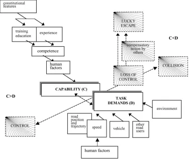
than capability, then the driver is in danger [8]. Figure 3.1, taken from [3], is a graphical

(23)

R. Fuller / Accident Analysis and Prevention 37 (2005) 461–472 465

speed, like driver competence, is subject to the influence of human factor variables.

2.2. Hierarchical nature of driver decision making

Some authors (such asAllen et al., 1971; Michon, 1985; van der Molen and Botticher, 1988; Hollnagel et al., 2004) have emphasized the hierarchical nature of driver decision-making, pointing out the distinctions between strategic de-cisions (route and timing of journey), tactical dede-cisions (manouvering) and operational decisions (executive acts). More recently, Laapotti et al. (2001) have added an even higher level, which pertains to ‘goals for life and skills for liv-ing’. These distinctions are retained in the TCI model where drivers can influence task demand by making choices in rela-tion to each of the factors, which influence it as well as their own speed. Thus, they can make purchase or hire decisions so as to drive a vehicle with particular features (such as ABS), they can select a particular route to a destination (avoiding high density or high speed motorways, for example) and a par-ticular time-of-day (avoiding periods of congestion or driv-ing in darkness—see, for example, Rimmo and Hakamies-Blomqvist, 2002). They can shift towards serial as opposed to parallel use of vehicle controls (Hakamies-Blomqvist et al., 1999) and they can also influence task demand by using di-rectional indicators (and other signals) to affect the behaviour

of other road users. Drivers also have some control over their capability, and decisions here also have a hierarchical struc-ture. Remotest from real-time decisions on the roadway are decisions regarding type, amount and level of training and about the kinds of driving experienced. Closer to real-time driving are decisions about exposure to a range of human fac-tor variables such as fatigue, stress and the effects of alcohol and of other drugs. And on an ongoing basis, drivers can vary their level of effort.

Putting all of these general features of the determinants of driver capability and task demand together, we arrive at the model presented inFig. 2. The elements of the model interact to determine task difficulty and the outcome for the driver in terms of whether or not control is maintained or lost.

2.3. The interaction between task demand and capability

The TCI model as presented inFig. 2gives the impression that task demand and capability are independent elements. However, it must be recognized that this is not necessarily, or even usually, the case. Capability is determined by many variables and one of these is the driver’s level of arousal or activation. The relationship between these two is tradition-ally described by an inverted U curve, with relatively lower levels of capability associated with both very low and very high levels of arousal. Arousal is partly determined by

en-Fig. 2. The task–capability interface model.

Figure 3.1: Task-capability interface model.

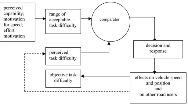
To complete the model, Fuller proposes the notion of task difficulty homeostasis. The

motivation behind task difficulty homeostasis is described by Fuller thusly:

The proposition I want to suggest is that at the outset of a journey, and

sometimes also during it, a driver will determine a range of task difficulty

that she/he is prepared to accept, a kind of target margin or envelope of task

difficulty. A key element of this is the upper boundary of difficulty beyond

(24)

place both choice of route and time of journey and, on an ongoing basis, will

influence speed choice. In fact, once the more strategic decisions have been

made, it will be speed choice, which the driver will predominantly use to

control the level of task difficulty experienced [3].

This idea of homeostasis is rooted in previous work of Wickens and Hollands [9] that

finds workers who have low workloads will tend of add jobs or overworked workers will

shed jobs to reach a more acceptable level of workload. Figure 3.2 from [3] demonstrates

the task difficulty homeostasis process.

R. Fuller / Accident Analysis and Prevention 37 (2005) 461–472 467

3. Task difficulty homeostasis

How might the perception of task difficulty determine driver behaviour? The proposition I want to suggest is that at the outset of a journey, and sometimes also during it, a driver will determine a range of task difficulty that she/he is prepared to accept, a kind of target margin or envelope of task difficulty. A key element of this is the upper bound-ary of difficulty beyond which the driver prefers not to go. That preference may influence in the first place both choice of route and time of journey and, on an ongoing basis, will influence speed choice. In fact, once the more strategic de-cisions have been made, it will be speed choice, which the driver will predominantly use to control the level of task dif-ficulty experienced (seeFig. 4), although as suggested by

Hakamies-Blomqvist et al. (1999), drivers may also change the ‘architecture’ of their performance. What determines the preferred level will be motivation for speed, perceived capa-bility and effort motivation. Motivation for speed arises from variables such as available time for a journey, possible social forces relating to passengers (e.g., desire to ‘show-off’ to peers or to provide a comfortable ride for an elderly person). Perceived capability will be a function of estimates of compe-tence and sensitivity to the effects of human factor variables. It is as if the driver asks herself/himself: what do I have to do here and what am I able to do? The result of this will be an acceptable, preferred range of task difficulty. This concept of task difficulty or workload homeostasis has been alluded to elsewhere in the context of industrial work. As stated by

Wickens and Hollands (2000): “Given some flexibility, op-erators usually work homeostatically to achieve an ‘optimal level’ of workload by seeking tasks when workload is low and shedding them when workload is excessive” (p. 470). In a self-paced task like driving, modifications of speed provide a very flexible and fairly rapid means of control of workload level (see also next section).

Task difficulty is an expression of the separation between task demand and driver capability. From a safety perspective, a key issue is their degree of separation. The closer

capabil-ity is to task demand, the more difficult will be the task and the less reserve capability there will be to accommodate a sudden increase in task demand (such as a child dashing out from behind a parked vehicle). This problem may be partic-ularly salient where journey time is limited, forcing a driver to drive faster than would otherwise be preferred (such as a truck driver attempting to make a just-in-time delivery). In such situations safety may be further challenged by the fact that capability may be simultaneously lowered by the stress of anticipated ‘mission failure’ and a state of height-ened anxiety. But the general principle proposed here is that drivers are motivated to maintain a preferred level of task dif-ficulty. Speed choice is the primary solution to the problem of keeping task difficulty within selected boundaries and, as de-scribed above, those boundaries are subject to motivational influences. This principle explains not only the continuous adjustment of speed to perceived hazards on the roadway (such as approaching a small radius bend) and the general phenomenon of behavioural adaptation (OECD, 1990) but also the effects on driver speed of traffic calming measures (such as throats, chicanes, lane narrowing and gateways).

Hoyos (1986), in discussing a study that measured driver estimates of task demand and their speed, reported that drivers used compensatory speed reductions as demand increased. In a study of the behaviour of older drivers, de Raedt and Ponjaert-Kristoffersen (2000)found that this kind of ‘tacti-cal’ compensation was associated with better drivers, as rated by driving instructors and by number of accidents. They con-cluded that it would be advisable to evaluate compensatory abilities in fitness-to-drive assessments of older drivers and recommended that older drivers should learn such strategies, as well as more ‘strategic’ decisions, such as avoiding high demand situations (driving in dark, fog, etc.). They also sug-gested, in line withHakamies-Blomqvist (1994)and the fun-damental postulate of the TCI model, that “it is probable that the immediate goal of compensation behaviour of older drivers is to reduce mental load, with increased safety a by-productrather than the main goal of the behaviour” (italics mine). In an interesting technical development from this line

Fig. 4. Task difficulty homeostasis.

Figure 3.2: Task difficulty homeostasis.

In summary, the Task-Capability Interface model attempts to describe the level of

danger that a driver is experiencing by considering human factors and the current driving

(25)

3.1.2 Comparison of Driver Models

Now that the TCI has been described, it can be compared with other models used to

study and predict driver behavior. From this comparison we can discover the TCI’s

strengths and weaknesses.

Researchers have employed many tools in their attempts to model driver behavior.

Some of the most notable modeling tools are neural networks, fuzzy logic, hybrid

dy-namical systems, etc. [10] [11] [2]. Each of these modeling strategies are used to achieve

the same goal of improving the safety of the driver, but their results are not universally

applicable. Many of these models are designed to predict specific tactical decisions like

collision avoidance and evaluation of driver skill, while some models take an entirely

different approach and attempt to model the driver’s cognitive process [1].

In summary, theTask-Capability Interface Model’s contribution to driver modeling is

its abdication of predicting tactical driver decisions. The TCI provides the researcher with

a metric to describe the situation that a driver is in and provides a way of determining

if a new tactical decision must be made. When the TCI is viewed in this manner, it can

be used to create a more complete safety-conscious model.

3.2 Implementing the Task-Capability Interface Model

Now that the TCI has been explained and justified, we can consider the heart of this

thesis: the implementation of the TCI. As was stated earlier, the model needs to be

understandable and accurate. In order to satisfy the criteria of understandability, a

fuzzy logic rules-based system was chosen and the membership functions were designed

heuristically. As for accuracy, data regarding driver behavior was found in journals [12]

(26)

In keeping with the research behind the Task-Capability Interface, three important

factors were identified from [8] and data collected from [12] and [13] was used to construct

the membership functions in the rule-based system. Sleepiness, rainfall, and speed were

the three factors chosen because of their ubiquitous nature and the availability of data

with respect to drivers.

For the purposes of implementation, the model was broken up into two smaller models:

the capability model and the demand model. The design of the two models will be

discussed herein.

3.2.1 Capability Model

In keeping with the research behind the TCI, it was decided that the Capability model

would be a single input single output system that depends on the sleepiness of the driver.

In order to simplify the creation of this model, key assumptions had to be made. In order

to make the model manageable, it is assumed that the driver is in good health and has

average training and experience. These assumptions allow the driver’s capability to be

determined solely by the “human factors” element shown in Figure 3.1. Sleepiness was

chosen because of the availability of data and the practicality of measurement.

In [13], researchers had car drivers rate their level of sleepiness on the Stanford

Sleepi-ness Scale, a scale ranging from 1 to 7, and found that drivers who had five or fewer hours

of sleep in the previous 24 hours had a significant increase in risk while driving. The first

step in creating the Capability model is transforming this data into fuzzy membership

functions.

The input membership functions were chosen to partition the level of sleepiness into

three categories: low, medium, and high. Figure 3.3 shows the three trapezoidal

(27)

membership functions were chosen in such a way as to err on the side of caution by

increasing the sleepiness of the driver.

Figure 3.3: Capability Input Membership Functions.

Table 3.1: Capability Input Membership Function Parameters

Name Point 1 Point 2 Point 3 Point 4

Low 0 0 1.452 3.23

Medium 2.01 2.9 3.341 4.65

High 3.786 4.86 7 7

The output membership functions were chosen to partition the driver’s capability into

three categories: low, medium, and high. Unlike the input membership functions, only

(28)

was chosen to be a triangle. Figure 3.4 shows the three membership functions and table

3.2 shows the membership function parameters. These shapes were chosen to reflect the

quick decline in driver capability.

Figure 3.4: Capability Output Membership Functions.

Table 3.2: Capability Output Membership Function Parameters

Low 0 0 0.03833 0.36

Medium 0.3241 0.48 0.578 NA

High 0.444 0.6045 1 1

Three rules were created to map the input to the output and they are listed

(29)

functions and the rules that tie them together.

1. If sleepiness is low then capability is high.

2. If sleepiness is medium then capability is medium.

3. If sleepiness is high then capability is low.

Figure 3.5: Capability Model Input-Output Mapping

The input-output mapping reflects the results of [13], where drivers exhibit increased

(30)

3.2.2 Demand Model

The Demand model was made to account for the effects that the driver experiences due to

the environment. In order to give the demand model greater flexibility, it was constructed

as a two-input single-output system. The two inputs are rainfall in hundredths of an inch

per hour and the car’s speed (as a percentage) relative to the speed limit.

Data for constructing the membership functions was taken from [12]. Researchers

partitioned the amount of rainfall into three different categories: no rain, light, and

heavy. Correspondingly, the input rainfall membership functions were chosen to be zero

(triangle), light (trapezoid), and heavy (trapezoid). Figure 3.6 shows the membership

functions and Table 3.3 contains the parameters for the rainfall membership functions.

Figure 3.6: Demand Rainfall Membership Functions.

In [12], it was found that drivers would slow down 5%-6.5% in light and heavy rain,

(31)

Table 3.3: Demand Rainfall Membership Function Parameters

Zero 0 0 6.071 NA

Light 4.2 6.06 11.07 16.26

Heavy 13.45 15 30 30

rain; this decision was supported by the Risk Homeostasis phenomenon discussed in [3].

The data for speed was used to create three membership functions: low (trapezoid),

normal (triangle), and high (trapezoid). Figure 3.7 contains the membership functions

associated with speed and Table 3.4 contains the membership function parameters.

(32)

Table 3.4: Demand Speed Membership Function Parameters

Low -6.41% -6.41% -4.663% -1.79%

Normal -3% 0% 2% NA

High 1% 3.04% 6.41% 6.41%

The output component of the Demand model was designed heuristically to couple no

rainfall and low speed with low demand, and to couple heavy rainfall and high speed

with high demand. Ultimately, the membership functions for the output were chosen

to partition the demand into three categories: low (triangle), medium (triangle), and

high (trapezoid). Figure 3.8 shows the membership functions and Table 3.5 contains the

(33)

Figure 3.8: Demand Output Membership Functions.

Table 3.5: Demand Output Membership Function Parameters

Low 0 0 0.4 NA

Medium 0.1 0.5 0.9 NA

High 0.64 0.8426 1 1

The rules that form the input-output mapping are as follows:

1. If rainfall is zero and speed is low then demand is low.

(34)

3. If rainfall is zero and speed is high then demand is medium.

4. If rainfall is light and speed is low then demand is medium.

5. If rainfall is light and speed is normal then demand is medium.

6. If rainfall is light and speed is high then demand is high.

7. If rainfall is heavy and speed is low then demand is medium.

8. If rainfall is heavy and speed is medium then demand is high.

9. If rainfall is heavy and speed is high then demand is high.

The input-output mapping that results from these rules is shown in Figure 3.9.

(35)

In total, this implementation of theTask-Capability Interfacedecreases the complexity

of Figure 3.1. Instead of considering eleven inputs, three were chosen. Figure 3.10

represents the new simplified TCI that is implemented herein.

Figure 3.10: Simplified Task-Capability Interface.

When implemented in Simulink, the model can provide “snapshots” of a situation

given all three inputs, or it can provide a “real-time” output if the inputs are described

as functions with respect to time. This allows the TCI to used as a component in a larger

(36)

Chapter 4 Sensitivity Analysis

After designing a model, we require a certain amount of analysis before its predictions

can be trusted. Sensitivity analysis provides the modeler with several tools to gain insight

into the model’s performance with respect to its parameters. Sensitivity analysis can be

broken down into three classes: screening methods, local SA methods, and global SA

methods [14, p. 10]; since local sensitivity analysis is the only method used in this thesis,

we will not discuss other methods. Local sensitivity analysis is used to determine the

local impact that parameters have on the output of a model and how variations of said

parameters affect the output [14, p. 10]. This method of analysis is used by modelers for

many different systems, including oil spills [15], fault analysis [16], etc.. Local SA can be

calculated several ways, but in this case we will use the Finite-Difference Approximation

(37)

4.1 Analysis of the TCI

Since local sensitivity analysis is computed as a finite difference, a way of accessing

and changing membership function parameters was needed. MATLAB’s Fuzzy Logic

Toolbox provides a data structure, called the Fuzzy Inference System, that allows the

user to change the desired membership function parameters and thus provides a method

of implementing the finite-difference approximation. It should be noted that since the

TCI is the linear combination of the output of two independent fuzzy systems, it was

decided that the two systems would be analyzed independently. This decoupling of

models has no impact on the overall results.

4.1.1 Choosing Inputs

Before the outputs can be calculated, we must choose an appropriate input with which

the model can be tested. The nature of the Fuzzy Inference System requires that several

different inputs be tested for each input set so that a more complete data set can be

generated. If, for instance, a trapezoidal membership function’s third parameter is being

analyzed and the parameter reshapes the membership function in such a way that the

fuzzy value corresponding to the input no longer changes, the output will no longer change

and no useful data will be generated. In other words, the output becomes constant and

the derivative will become zero, resulting in a sensitivity of zero. Therefore we must

choose inputs that have values close to that of the membership function parameters that

(38)

Figure 4.1: The inputx= 1.2 generates no new information after the parameter increases

in value.

It was ultimately decided that three different inputs would be chosen for each

mem-bership function and the values of these inputs were chosen based on the value of the

membership function parameter in question.

4.1.2 Computing Model Output

In order to compute the finite-difference approximation, we must choose the parameter

that we wish to vary, how much we will vary the parameter at each iteration, and what

input we will use. It was decided that when performing sensitivity analysis on a fuzzy

(39)

be chosen and those parameters would be perturbed around their original value, i.e.

±5%. After the output is stored, the sensitivity is calculated using the finite-difference

approximation. While two different functions are used to analyze the parameters in input

sets and output sets, the algorithm remains the same. Shown below is the algorithm in

MATLAB to analyze the ith _{membership function parameter.}

Algorithm 1Parameter perturbation algorithm

max←1.05∗pi

min←0.95∗pi

paramDistance←max−min

for k = 0 : ∆p:paramDistance do if mf(i) + ∆p < max then

mf(i)←mf(i) + ∆p

else

mf(i)←max

end if

output(k)←evalf is(f isInput)

end for

4.1.3 Calculating Local Sensitivity

Once the data gathered by the parameter perturbation algorithm is ready, the local

sensitivity analysis can be performed by computing the value of the derivative using

the finite-difference approximation. The Finite-Difference Approximation is computed

thusly,

∂y

∂kj

≈ y(kj + ∆kj)−kj

∆kj

, j = 1, . . . , m.

whereyis the output,kj is thejthmembership function parameter of thekthmembership

(40)

4.2 Sensitivity Data

The sensitivity analysis of the Task-Capability Interface is broken down in two ways;

first, the analysis of the capability model and the demand model are separated, and

secondly the input membership function parameter analysis and output membership

function parameter analysis are separated from one another. Herein the data will be

presented in accordance with the previous breakdown.

4.2.1 Capability Model Sensitivity Data

The capability model consists of three input membership functions and three output

membership functions. In total, there are seven membership function parameters. The

four input membership function parameters tested are SL1, SL2, SL3, SL4. The

remain-ing parameters correspond to the model’s output and they are C1, C2, and C3. All

(41)

Figure 4.2: Capability Model Membership Functions.

The figures 4.3 through 4.9 and tables 4.1 and 4.2 contain all of the data gathered for

the driver Capability model. Included in the data is the parameter name, system input

(42)

(43)

(44)

(45)

(46)

Table 4.1: Sleepiness Membership Function Parameter Sensitivity

Parameter Input Maximum Value Minimum Value

SL1 1.45 0.0198 0

2.5 0.0405 0

3.2 0.0102 0

SL2 2.6 0.0434 3.8284×10−15

2.9 0.0157 0

3 0.0042 0

SL3 3.34 0.0015 0

4.3 0.0479 1.6615×10−15

4.6 0.0140 8.3076×10−16

SL4 4.4 0.0644 0

4.86 0.260 0

(47)

(48)

(49)

(50)

Table 4.2: Capability Output Membership Function Parameter Sensitivity

C1 4.3 0.0113 0

4.6 0.0823 0

5.5 0.0707 0

C2 2.3 0.0687 0

4.1 0.1055 0.0660

4.5 0.0232 0.0088

C3 1 0.2291 0.2137

2 0.1651 0.1544

2.5 0 0

4.2.2 Demand Model Sensitivity Data

The demand model consists of nine membership functions, six dedicated to the input and

three dedicated to the output. The sensitivity analysis is performed on nine membership

function parameters. The rainfall parameters are R1, R2, and R3. The speed parameters

are S1, S2, and S3. Lastly, the demand parameters are D1, D2, and D3. Figure 4.10

shows the input membership functions with labeled parameters and Figure 4.11 shows

(51)

(52)

Figure 4.11: Demand Model Output Membership Functions.

The figures 4.12 through 4.20 and tables 4.3, 4.4, and 4.5 contain the sensitivity data

for the driver Demand model. The information is presented in the same fashion as the

(53)

(54)

(55)

(56)

Table 4.3: Rainfall Membership Function Parameter Sensitivity

R1 (5.5,3) 0.0464 0

(6.1,3) 0.0172 0

(6.5,3) 0 0

R2 (10.5,0) 0 0

(11.07,0) 2.0058×10−15 0

(12,0) 4.0116×10−15 0

R3 (14,0) 0.0921 0

(15,0) 0.0542 0

(57)

(58)

(59)

(60)

Table 4.4: Speed Membership Function Parameter Sensitivity

S1 (0,-4.66) 0.0052 0

(0,-3.2) 0.0145 0

(0,-3.7) 0.0145 0

S2 (0,-1) 5.5511×10−15 ₀

(0,1) 6.6613×10−15 0

(0,1.5) 7.7716×10−15 0

S3 (0,2.5) 2.1912×10−14 ₀

(0,3) 7.3041×10−15 ₀

(61)

(62)

(63)

(64)

Table 4.5: Demand Output Membership Function Parameter Sensitivity

D1 (3,-1) 0 0

(5,4) 0 0

(12.5,4) 0 0

D2 (10,-1) 0.2819 0

(15,-2) 0.0590 0

(20,6) 0 0

D3 (7,-3) 0 0

(12.5,2) 0.1130 0

(65)

Chapter 5 Results of Model Analysis

To aid in the interpretation of the model’s behavior, it was decided that a new metric

was needed to examine the magnitude of the change in output as a percentage. This

new metric was inspired from the percent error calculation commonly used in physics

and chemistry to quantify error present in experiments.

% error = |Theoretical value - Experimental value|

Theoretical value ∗100%

In order to quantify the changes in output over the range of parameter values used in

the sensitivity calculations, we change the percent error calculation thusly, wherepmin is

the model’s output calculated with the minimum parameter value, pmax is the model’s

output calculated with the maximum parameter value, and poriginal is the output value

(66)

Pmax =

|pmax−poriginal|

poriginal

∗100% (5.1)

Pmin =

|pmin−poriginal|

poriginal

∗100% (5.2)

Ptotal =

|pmax−pmin|

poriginal

∗100% (5.3)

Lastly, we will consider the case of capability and demand having values close to one

another. In particular, we will examine the inputs that lead to this situation and what

implications these inputs have for the model and driver safety.

5.1 Capability Model

5.1.1 Sleepiness

There are four membership function parameters in the sleepiness input under

consid-eration when analyzing the sensitivity of the capability model. The following sections

contain the data found for each of the four parameters along with conclusions that can

be drawn from the gathered data.

SL1

Parameter SL1 of the “low” membership function was tested with the inputs I1 = 1.45,

I2 = 2.5, and I3 = 3.2. Table 5.1 contains the data found with the previously listed

inputs.

From examination of the data below, we can see that the capability model is most

(67)

percentage change, the output does not vary appreciably for any of the inputs used in

sensitivity calculations. Note that Savg is the average sensitivity calculated for a fixed

input.

Table 5.1: SL1 Analysis Results

I1 = 1.45 I2 = 2.5 I3 = 3.2

Savg 0.0190 0.0416 0.0108

Pmax 0% 0.3804% 0.1495%

Pmin 0.1447% 0.4545% 0.1743%

Ptotal 0.1447% 0.8349% 0.3237%

SL2

Parameter SL2 of the “medium” membership function was tested with the inputs I1 =

2.6,I2 = 2.9, and I3 = 3.

When changing the parameter SL2, it was found that the model was most sensitive

when the input is in the neighborhood of 2.6. Perturbing SL2 resulted in relatively small

changes according to the Pmax and Pmin metrics. Ultimately it can be concluded that

(68)

I1 = 2.6 I2 = 2.9 I3 = 3

Savg 0.0546 0.0147 0.0039

Pmax 1.0615% 0.4144% 0.0636%

Pmin 1.1997% 0.0402% 0%

Ptotal 2.2611% 0.4547% 0.0636%

SL3

Parameter SL3 of the “medium” membership function was tested with the inputs I1 =

3.34, I2 = 4.3, and I3 = 4.6.

The capability model is most sensitive, with respect to SL3, when the input is in the

neighborhood of 4.3. The change in output found while perturbing SL3 is significant.

I1 = 3.34 I2 = 4.3 I3 = 4.6

Savg -0.0046 0.0340 0.0098

Pmax 0% 2.3319% 1.1492%

Pmin 0.1486% 2.5870% 1.1510%

(69)

SL4

Parameter SL4 of the “high” membership function was tested with the inputs I1 = 4.4,

I2 = 4.86, and I3 = 5.

The maximum sensitivity resulting from changes in SL4 is found when the input is

in the neighborhood of 4.4. Additionally, it is found that perturbations of SL4 result in

the largest changes in model output. It can be concluded that changes in the value of

SL4 can have a significant impact in the capability model.

I1 = 4.4 I2 = 4.86 I3 = 5

Savg 0.0560 0.0205 0.0142

Pmax 4.8824% 4.1294% 1.7569%

Pmin 7.0562% 0.8855% 0%

Ptotal 11.9386% 5.0150% 1.7569%

5.1.2 Capability

The following sections contain the results found while analyzing the sensitivity of the

capability model with respect to three of the output membership function parameters.

As with the previous section concerning the sleepiness parameters, we attempt to draw

(70)

C1

Parameter C1 of the “low” membership function was tested with the inputs I1 = 4.3,

I2 = 4.6, and I3 = 5.5.

The capability model is found to be most sensitive, with respect to output parameter

C1, when the input is in the neighborhood of 4.6. Analysis of the output shows that

perturbations of C1 do not result in a significant change in model output.

Table 5.5: C1 Analysis Results

I1 = 4.3 I2 = 4.6 I3 = 5.5

Savg 0.0127 0.0821 0.0637

Pmax 0.0085% 0.0892% 0.0841%

Pmin 0.0105% 0.1109% 0.1018%

Ptotal 0.0190% 0.2000% 0.1018%

C2

Parameter C2 of the “medium” membership function was tested with the inputsI1 = 2.3,

I2 = 4.1, and I3 = 4.5.

The capability model is found to be most sensitive, with respect to C2, when the input

is in the neighborhood of 4.1. Given the value ofSavg and the percentage deviations, the

(71)

I1 = 2.3 I2 = 4.1 I3 = 4.5

Savg 0.0891 0.0900 0.0099

Pmax 0.1713% 0.5760% 0.1056%

Pmin 0.1416% 0.4100% 0.0737%

Ptotal 0.3129% 0.9859% 0.1793%

C3

Parameter C3 of the “high” membership functions was tested with the inputs I1 = 1,

I2 = 2, and I3 = 2.5.

Sensitivity analysis shows that the model is most sensitive with respect to C3 when

the input is in the neighborhood of 1. The percentage change found is small, but not

negligible; this suggests that small changes to C3 do affect model output to a small

degree.

I1 = 1 I2 = 2 I3 = 2.5

Savg 0.2196 0.1597 0.0133

Pmax 0.8570% 0.6358% 0.0631%

Pmin 0.7100% 0.5204% 0.0481%

(72)

5.1.3 Analysis Summary

In summary, changes to the values of membership function parameters SL3 and SL4

resulted in the largest deviations in model output. Since driver capability should drop

significantly as the driver becomes more sleepy, this result makes heuristic sense.

Addi-tionally, it can be seen in Table 5.3 and Table 5.4 that the largest changes occur when the

parameter values become smaller. In the case of SL3, the capability will decrease for an

input value equal to or greater than the original parameter value as the value decreases.

The large change in output that results from decreasing the value of SL4 comes from the

increased membership values that nearby inputs assume.

5.2 Demand Model

5.2.1 Rainfall

The sensitivity analysis data and the respective conclusions concerning three of the

rain-fall membership function parameters are contained in the following section.

R1

Parameter R1 from the “light” membership function was tested with the inputs I1 =

(5.5,3), I2 = (6.1,3), and I3 = (6.5,3).

The demand model is found to be most sensitive to changes in R1 when the rainfall

input is in the neighborhood of 5.5. The change in model output is small when perturbing

(73)

Table 5.8: R1 Analysis Results

I1 = (5.5,3) I2 = (6.1,3) I3 = (6.5,3)

Savg -0.0424 -0.0154 0

Pmax 1.2785% 0.4337% 0%

Pmin 1.7650% 0% 0%

Ptotal 3.0435% 0.4337% 0%

R2

Parameter R2 from the “light” membership function was tested with the inputs I1 =

(10.5,0), I2 = (11.07,0), and I3 = (12,0).

Given the magnitude of the results found while testing the sensitivity of the demand

model with respect to R2, it can be concluded that small changes to this parameter have

no effect on the model.

I1 = (10.5,0) I2 = (11.07,0) I3 = (12,0)

Savg 0 -5.0146×10−14 0

Pmax 0% 0% 0%

Pmin 0% 2.2204×10−14% 0%

(74)

R3

Parameter R3 from the “heavy” membership function was tested with the inputs I1 =

(14,0), I2 = (15,0), and I3 = (15.5,0).

The demand model is found to be most sensitive to a rainfall input of 14 while

perturbing R3. Changes in R3 can have significant effect on the model’s output when

the rainfall input is not a full member of the “heavy” membership function.

I1 = (14,0) I2 = (15,0) I3 = (15.5,0)

Savg -0.0524 -0.0410 -0.0310

Pmax 3.3984% 4.0432% 1.2234%

Pmin 9.0251% 1.1446% 0%

Ptotal 12.423% 5.1878% 1.2234%

5.2.2 Speed

Data and conclusions regarding the effects of the three Speed membership function

pa-rameters are contained in the following section.

S1

Parameter S1 from the “low” membership function was tested with the inputs I1 =

(0,−4.66), I2 = (0,−3.2), I3 = (0,−3.7).

(75)

the range of -3.7. As evidenced by the percentage change, the model output does not

strongly depend on the value of S1.

Table 5.11: S1 Analysis Results

I1 = (0,−4.66) I2 = (0,−3.2) I3 = (0,−3.7)

Savg -0.0029 -0.0130 -0.0138

Pmax 0% 1.6906% 1.8766%

Pmin 0.5206% 1.8829% 2.2252%

Ptotal 0.5206% 3.5735% 4.1018%

S2

Parameter S2 from the “normal” membership function was tested with the inputs I1 =

(0,−1), I2 = (0,1), andI3 = (0,1.5).

As can be seen in Table 5.12, the model is essentially insensitive to small changes in

(76)

I1 = (0,−1) I2 = (0,1) I3 = (0,1.5)

Savg -3.4694×10−16 6.1679×10−17 -1.5543×10−15

Pmax 1.3323×10−13% 3.3307×10−14% 9.992×10−14%

Pmin 7.7716×10−14% 2.2204×10−14% 2.5535×10−14%

Ptotal 5.5511×10−14% 1.1102×10−14% 1.5543×10−13%

S3

Parameter S3 of the “high” membership function was tested with the inputsI1 = (0,2.5),

I2 = (0,3), andI3 = (0,3.1).

The sensitivity of the model, with respect to S3, is similar to the sensitivity of the

model with respect to S2 in that changes to the value of S3 exhibit little to no sensitivity

in the model and little to no change in model output.

I1 = (0,2.5) I2 = (0,3) I3 = (0,3.1)

Savg -3.9443×10−31 0 0

Pmax 0% 2.2204×10−14% 0%

Pmin 0% 2.2204×10−14% 0%

(77)

5.2.3 Demand

The following section contains the data and conclusions gathered from the analysis of

three membership function parameters in the demand model output.

D1

Parameter D1 of the “low” membership function was tested with the inputsI1 = (3,−1),

I2 = (5,4), andI3 = (12.5,4).

Table 5.14 shows that the demand model is insensitive to small changes in the value

of D1 and that changes to D1 do not affect the output.

Table 5.14: D1 Analysis Results

I1 = (3,−1) I2 = (5,4) I3 = (12.5,4)

Savg 0 0 0

Pmax 0% 0% 0%

Pmin 0% 0% 0%

Ptotal 0% 0% 0%

D2

Parameter D2 of the “medium” membership function was tested with the inputs I1 =

(10,0), I2 = (15,−2), and I3 = (20,6).

The demand model is most sensitive to changes in the value of D2 when the input is

(78)

a small change in the output.

I1 = (10,0) I2 = (15,−2) I3 = (20,6)

Savg 0.2777 0.0556 0

Pmax 1.112% 0.1843% 0%

Pmin 1.381% 0.2265% 0%

Ptotal 2.493% 0.4107% 0%

D3

Parameter D3 of the “high” membership function was tested with the inputsI1 = (7,−3),

I2 = (12.5,2), and I3 = (20,6).

The model is most sensitive to changes in the value of D3 when the input is in the

neighborhood of (20,6), however, the output does not change significantly with small

(79)

I1 = (7,−3) I2 = (12.5,2) I3 = (20,6)

Savg 0 0.1077 0.1702

Pmax 0% 0.4195% 0.6093%

Pmin 0% 0.5448% 0.8772%

Ptotal 0% 0.9642% 1.4865%

5.2.4 Analysis Summary

After performing sensitivity analysis, the data shows that the demand model is most

affected by changes in the parameters R3 and S1. The most significant change in model

output occurs when the “heavy” rainfall membership function’s core is widened. Since a

heavy rainfall should have a significant negative impact in a driving scenario, this result

is heuristically sound. Changes to R2, S2, S3, and D1 were found to have no impact on

model output.

5.3 Borderline Inputs

Referring back to Section 3.1.1, there is a discussion concerning the two cases ofC > D

andD > C. In addition to these two cases, there is a third case of interest: C ≈D. When capability is significantly greater than demand, it is clear that no corrective action must be

taken, and when demand is significantly greater than capability, it is clear that corrective

action must be taken; what is not clear is if any action is necessary when capability and

(80)

expect drivers to spend a significant portion of their time in this ambiguous region. To

aide in the discussion of this region of ambiguity, we will name it the “borderline region.”

Since the driver’s actions in this borderline region are beyond the scope of this thesis,

we will investigate the inputs that map into the borderline region. It was decided that

the borderline region would be defined as the set of outputs generated by the TCI where

the Demand model’s output value is within ten percent of the Capability model’s output

value. It was decided that the borderline region would be defined by a ten percent buffer,

as opposed to a strict equality between capability and demand, due to computational

and safety concerns; by relaxing the equality requirement we allow for a safety margin of

sorts.

To find the set of inputs that map to the borderline region, each input component,

rainfall, speed, and sleepiness, is divided into 100 uniformly partitioned values,

result-ing in 1,000,000 different input combinations tested; of the inputs tested, 72,184 inputs

mapped into the borderline region. Figure 5.1, Figure 5.2, and Figure 5.3 all show the

inputs that map into the borderline region.

Inspection of the inputs reveals that a significant portion of the input space maps

to the borderline region. We find that the majority of borderline inputs exist when the

sleepiness component has a value between three and four. Rainfall inputs near 0.05”

rain/hour define a wall between the “safe” region and the “dangerous” region.

Examina-tion of the affects of the speed input reveals a box-like region where inputs arounds 0%

are still safe, but more positive speeds result in a quick transition to “dangerous” inputs.

In essence, we can see that these inputs occur in situations tend to occur in scenarios

where a driver appears to be moving into a dangerous region of operation and the driver

must be vigilant, as their margin for error is likely to be diminishing. When viewed

(81)

the intentions with which the model was designed.

(82)

(83)

(84)

Chapter 6 Conclusion

The purpose of this thesis was to design, implement, and analyze a model intended to

be used as a metric for automobile driver safety. In order to avoid the complexities

associated with approaches that make use of tactical driver simulators, we chose to go in

a direction that considered the driver and their environment from a holistic viewpoint.

The model chosen to satisfy these requirements was the Task-Capability Interface. The

TCI is a model based on the concepts of task demand, task capability, and task difficult

homeostasis written about by Ray Fuller in [3]. In this thesis the TCI’s complexity

was reduced by considering a reduced set of input factors; additionally, the model was

implemented as a fuzzy logic rules-based system to maintain a simple model architecture.

After surveying the available data, it was decided that the three input factors for

the TCI would be driver sleepiness, rainfall, and automobile speed relative to the posted

speed limit. Sleepiness was chosen to determine driver capability, rainfall was chosen

as a demand input to represent a significant factor outside of the driver’s control, and

relative speed was chosen as a demand input to give the driver an element of control.

Implementation and Sensitivity Analysis of a Task-Capability Interface Model for Automobile Driver Safety.

ABSTRACT

DEDICATION

BIOGRAPHY

ACKNOWLEDGEMENTS

TABLE OF CONTENTS

LIST OF TABLES

LIST OF FIGURES

Chapter 1

Introduction

Chapter 2

Fuzzy Sets, Fuzzy Logic, and

Modeling

2.1

Set Theories

2.1.1

Zermelo-Fraenkel Set Theory

2.1.2

Fuzzy Set Theory

2.2

Fuzzy Logic

2.3

Modeling with Fuzzy Sets and Fuzzy Logic

2.3.1

Rule-Based Systems

2.3.2

Step 1: Fuzzification of Inputs

2.3.3

Step 2: Application of Fuzzy Operator

2.3.4

Step 3: Application of Implication Method

2.3.5

Step 4: Aggregation of Rules

2.3.6

Step 5: Defuzzification

Chapter 3

Modeling Driver Capability and

Task Demand

3.1

Task-Capability Interface Model

3.1.1

Philosophy of the TCI

3.1.2

Comparison of Driver Models

3.2

Implementing the Task-Capability Interface Model

3.2.1

Capability Model

3.2.2

Demand Model

Chapter 4

Sensitivity Analysis

4.1

Analysis of the TCI

4.1.1

Choosing Inputs

4.1.2

Computing Model Output

4.1.3

Calculating Local Sensitivity

4.2

Sensitivity Data

4.2.1

Capability Model Sensitivity Data

4.2.2

Demand Model Sensitivity Data

Chapter 5

Results of Model Analysis

5.1

Capability Model

5.1.1

Sleepiness

5.1.2

Capability

5.1.3

Analysis Summary

5.2

Demand Model

5.2.1

Rainfall