| INVESTIGATION
Quantifying GC-Biased Gene Conversion in Great Ape
Genomes Using Polymorphism-Aware Models
Rui Borges,* Gergely J. Szöllosi,} †and Carolin Kosiol*,‡,1
*Institut für Populationsgenetik, Vetmeduni Vienna, 1210 Wien, Austria,†Department of Biological Physics, MTA-ELTE“Lendulet”
Evolutionary Genomics Research Group, Eötvös University, Pázmány P. stny. 1A, Budapest H-1117, Hungary, and‡Centre for Biological Diversity, School of Biology, University of St Andrews, Fife KY16 9TH, UK ORCID IDs: 0000-0002-5905-3778 (R.B.); 0000-0002-8556-845X (G.J.S.); 0000-0002-3219-6648 (C.K.)
ABSTRACTAs multi-individual population-scale data become available, more complex modeling strategies are needed to quantify genome-wide patterns of nucleotide usage and associated mechanisms of evolution. Recently, the multivariate neutral Moran model
was proposed. However, it was shown insufficient to explain the distribution of alleles in great apes. Here, we propose a new model
that includes allelic selection. Our theoretical results constitute the basis of a new Bayesian framework to estimate mutation rates and
selection coefficients from population data. We apply the new framework to a great ape dataset, where we found patterns of allelic
selection that match those of genome-wide GC-biased gene conversion (gBGC). In particular, we show that great apes have patterns
of allelic selection that vary in intensity—a feature that we correlated with great apes’distinct demographies. We also demonstrate that
the AT/GC toggling effect decreases the probability of a substitution, promoting more polymorphisms in the base composition of great
ape genomes. We further assess the impact of GC-bias in molecular analysis, andfind that mutation rates and genetic distances are
estimated under bias when gBGC is not properly accounted for. Our results contribute to the discussion on the tempo and mode of gBGC evolution, while stressing the need for gBGC-aware models in population genetics and phylogenetics.
KEYWORDSMoran model; boundary mutations; allelic selection; great apes; GC-bias; gBGC
T
HE field of molecular population genetics is currently being revolutionized by progress in data acquisition. New challenges are emerging as new lines of inquiry are posed by increasingly large population-scale sequence data (Casillas and Barbadilla 2017). Mathematical theory describ-ing population dynamics was developed before molecular sequences were available (e.g., Fisher 1930; Wright 1931; Moran 1958; Kimura 1964); now that ample data are avail-able to perform statistical inference, many models have been revisited. Recently, the multivariate Moran model with boundary mutations was developed and applied to exome-wide allele frequency data from great ape populations(Schrempf and Hobolth 2017). However, drift and mutation are not fully sufficient to explain the observed allele counts (Schrempf and Hobolth 2017). It was hypothesized that other forces, such as directional selection and GC-biased gene conversion (gBGC), may also play a role in shaping the dis-tribution of alleles in great apes.
Directional selection and gBGC have different causes but similar signatures: under directional selection, the advanta-geous allele increases as a consequence of differences in survival and reproduction among different phenotypes; under gBGC, GC alleles are systematically preferred. gBGC is a recombination-associated segregation bias that favors GC-alleles (hereafter, strong alleles) over AT-alleles (hereaf-ter, weak alleles) during the repair of mismatches that occur within heteroduplex DNA during meiotic recombination (Marais 2003). gBGC has been studied in several taxa includ-ing mammals (Duret and Galtier 2009; Romiguieret al.2010; Lartillot 2013), birds (Websteret al.2006; Weberet al.2014; Smedset al.2016; Corcoranet al.2017), reptiles (Figuetet al.
2015), plants (Muyleet al.2011; Serres-Giardiet al.2012; Clémentet al.2017; Liuet al.2018), and fungi (Pessiaet al.
Copyright © 2019 by the Genetics Society of America doi:https://doi.org/10.1534/genetics.119.302074
Manuscript received September 13, 2018; accepted for publication May 20, 2019; published Early Online May 30, 2019.
Available freely online through the author-supported open access option.
Supplemental material available at FigShare:https://doi.org/10.6084/m9.figshare. 8180960.
1Corresponding author: Centre for Biological Diversity, University of St Andrews,
2012; Lesecqueet al.2013; Liuet al.2018). However, apart from some studies in human populations (Katzman et al.
2011; Gléminet al.2015; Pouyetet al.2018), a population-level perspective of the intensity and diversity of patterns of gBGC among closely related populations is still lacking.
Several questions remain open regarding the tempo and mode of gBGC evolution. For example, the effect of demog-raphy on gBGC is still controversial. While theoretical results and studies in mammals and birds advocate a positive re-lationship between the effective population size and the in-tensity of gBGC (Nagylaki 1983; Romiguier et al. 2010; Weberet al.2014), Galtieret al.(2018) failed to detect such relationship between animal phyla. These results open the question as to which extent demography shapes the intensity of gBGC in closelyvs.distantly related species/populations. Another aspect that is not completely understood is the im-pact of GC-bias on the base composition of genomes (Phillips
et al.2004; Romiguieret al.2013). In particular, the
individ-ual and joint effect of gBGC and mutations shaping the sub-stitution process remains elusive. Here, we address these two questions by revisiting great ape data (Prado-Martinezet al.
2013) with a Moran model that accounts for allelic selection. The Moran model (Moran 1958) has a central position in describing the evolution of a population in that it models the dynamics of allele frequency changes in afinite haploid pop-ulation. Recently, an approximate solution for the multi-variate Moran model with boundary mutations (i.e., low mutation rates) was derived (Schrempf and Hobolth 2017). In particular, the stationary distribution was shown useful to infer population parameters from allele frequency data (Schrempfet al.2016; Schrempf and Hobolth 2017). Here, we present the Moran model with boundary mutations and allelic selection, derive the stationary distribution, and build a Bayesian framework to estimate population parameters. While De Maioet al.(2013) had previously proposed a Moran model with allelic selection, we introduce further assump-tions on the mutation scheme that permit us to mechanisti-cally describe the relative importance and impact of the population processes mediating the base composition of ge-nomes and expected divergence.
Other approaches making use of allele frequency data to estimate mutation rates and selection coefficients have been proposed in the literature. Gléminet al.(2015) proposed a method to quantify gBGC from the derived allele frequency spectra that incorporates polarization errors, takes spatial heterogeneity into account, and jointly estimates mutation bias. The number of derived alleles is modeled by a Poisson distribution on the mutation rates among weak, strong, and neutral alleles (Muyleet al.2011). Our approach differs from that of Gléminet al.(2015) as it does not require polarized data or need to account for polarization errors. In addition, our method makes use of the information given by thefixed sites—information that is usually discarded by other methods (Gléminet al.2015 included).
Furthermore, our application to great apes shows that most great apes have patterns of allelic selection consistent with
gBGC. Our results suggest further that demography plays a major role in determining the intensity of gBGC among great apes, as the intensity of the obtained selection coefficients correlates significantly with the effective population size of great apes. We also show that not accounting for GC-bias may considerably distort the reconstructed evolutionary process, as mutation and substitution rates are estimated under bias.
Methods
The multivariate Moran model with allelic selection
The modeling framework defined in this work builds on the model described by Schrempfet al.(2016), which, according to some proposed terminology (Vogl and Bergman 2015; Schrempf and Hobolth 2017), can be addressed as the mul-tivariate Moran model with boundary mutations (hereafter,
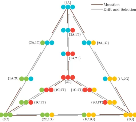
MM). Here, we describe theMMand allelic selection (here-after, MS). The multivariate Moran model can be also re-ferred to as a polymorphism-aware phylogenetic model (PoMo) if we consider the four-variate case (De Maioet al.
2013, 2015; Schrempfet al.2016),i.e., representing the four nucleotide bases (Figure 1).
Consider a haploid population ofNindividuals and a single locus withKalleles:aiandajare two possible alleles. The
population is monomorphicfNaig,i.e., theNindividuals have
the alleleai; differently, if two alleles are present in the
pop-ulation, the population is polymorphic fnai;ðN2nÞajg,
meaning that n individuals have the alleleai and ðN2nÞ
have the alleleaj.n=Nis therefore the frequency of alleleai
in the population.
Allele trajectories are given by the rate matrix Q. Time is accelerated by a factor ofN, and, therefore, instead of de-scribing Moran dynamics in terms of Moran events (Moran 1958), we developed a continuous version in which time is measured as the coalescent in generation time (in units ofN). Drift is defined by the neutral Moran model: the transition rates of the allelic frequency shifts depend only on the allele frequency, and are therefore equal regardless of allele in-creases or dein-creases in the population (Durrett 2008).
qfnai;ðN2nÞajg/fðnþ1Þai;ðN2n21Þajg
¼qfnai;ðN2nÞajg/fðn21Þai;ðN2nþ1Þajg¼nðN2nÞ
N : (1)
We accommodated mutation and selection in the framework of the neutral Moran model by assuming them to be decoupled (Baake and Bialowons 2008; Etheridgeet al.2010).
Mutation is incorporated based on a boundary mutation model, in which mutations occur only in the boundary states.
The boundary mutations assumption is met if the muta-tion rates maiaj are small (and N is not too large). More
specifically, by comparing the expectations of the diffusion equation with the polymorphic diversity under the Moran model, Schrempfet al.(2016) established thatNmaiajshould
be lower than 0.1. In fact, most eukaryotes fulfill this con-dition [see Lynch et al. (2016) for a review of mutation rates]. Another assumption of our boundary mutation model is that the polymorphic states can only be biallelic. However, this assumption is not a significant constraint as tri-or-more allelic sites are rare in sequences with low mu-tation rates.
We employed the strategy used by Burden and Tang (2016), and separated our model into a time-reversible and aflux part. We wrote the mutation rates as the entries of a specific mutation model, the general time-reversible model (GTR) (Tavaré 1986):maiaj¼raiajpaj¼rajaipaj, wherer
rep-resents the exchangeabilities between any two alleles ,andp the allele base composition (Equation 2). Here, we restricted ourselves to the GTR, as this model simplifies obtaining for-mal results (Burden and Tang 2016). Becausep hasK21 free parameters, andrincludes the exchangeabilities for all the possible pairwise combinations ofKalleles, we ended up having KðKþ1Þ=221 free parameters in the GTR-based boundary mutation model.
Until now, we have essentially described the model pro-posed by Schrempf et al. (2016); this work extends this model by including allelic selection. We modeled allelic selection by defining K21 relative selection coeffi -cients s: the selection coefficient of an arbitrary allele (A in our experiments) is fixed to 0. The selection coeffi -cients defined this way guarantee that our multi-allelic model behaves neutrally only under the condition that all the selection coefficients are the same and equal to 0. De-fining thefitness as the probability that an offspring of allele
ai is replaced with probability 1þsai (Durrett 2008), we
can formulate the component of allelic selection alongside with drift, and thus among the polymorphic states (Equa-tion 2).
Altogether, the instantaneous rate matrixQof the multi-variate Moran model with boundary mutations and allelic selection can be defined as
where uand v represent a frequency change in the allele counts (thoughNremains constant). The diagonal elements are defined by the mathematical requirement such that the respective row sum is 0.
As the parameters of the population size, mutation rate, and selection coefficients are confined, it is possible to scale them down to a small value ofNwhile keeping the overall dynamics unchanged (Appendix A). The virtual population sizeNbecomes a parameter describing the number of bins the allele frequencies can fall into. As a result, we can think ofN
either as a population size or a discretization scheme.
The stationary distribution
The stationary distribution of a Markov process can be obtained by computing the vectorcsatisfying the condition
qfuai;ðN2uÞajg/fvai;ðN2vÞajg¼
maiaj¼raiajpaj u¼N;v¼N21 majai¼raiajpai u¼0;v¼1 n
NðN2nÞð1þsaiÞ u¼n;v¼nþ1;0,n,N
n
NðN2nÞð1þsajÞ u¼n;v¼n21;0,n,N
0 ju2vj.1
; 8
> > > > > > > > > > < > > > > > > > > > > :
cQ¼0(Appendix B).cis the normalized stationary vector, and has the solution
kis the normalization constant
k¼X
ai2A
paið1þsaiÞN21
þ X
aiaj2AC
X
N21
n¼1
paipajraiajð1þsaiÞn21ð1þsajÞN2n21 N
nðN2nÞ;
(4)
whereAis the alphabet of theKallelesfa1;...;aKg, representing
the monomorphic states, andACall the possible pairwise combi-nations ofArepresenting theKðK21Þ=2 types of polymorphic statesfa1a2,a1a3,. . .,aK21aKg. For example, for the
four-multivariate case, we writeAas the alphabet of the four nucle-otide basesfA;C;G;TgandACas all the possible pairwise com-binations of the four nucleotide basesfAC;AG;AT;CG;CT;GTg.
For a population of sizeN, we have 4þ6ðN21Þpossible states, four of which are monomorphic (Figure 1).
Expected number of Moran events
From .Q. and c, we can compute the expected number of Moran events (mutations, drift, and selection) or the expected divergence per unit of time (in generations) under theMSmodel (Appendix C):
dMS¼2
k
X
aiaj2AC
XN
n¼1
pairaiajpajð1þsaiÞ n21ð
1þsajÞN2n: (5)
The quantity (5) can also be interpreted as the overall rate of the model. The expected number of Moran events for the neutral model can be easily calculated by lettings/0. To compare the Moran distancedMSwith the standard models of evolution, we
recalculated the Moran distance to account only for substitutions
eventsd*
MS: we correcteddMSby the probability of a mutation and
subsequentfixation under the Moran model (Appendix D)
d*
MS¼
2
k
X
aiaj2AC
paipajraiajð1þsaiÞNð1þsajÞN PN
n¼1ð1þsajÞ
nð
1þsaiÞN2nþ1: (6)
Bayesian inference with stationary distribution
We can define a likelihood function based on the stationary distribution for a set ofSindependent sites inNindividuals by taking the product ofcx over counts of monomorphic and
polymorphic sitescðxÞ, thus:
We employed a Bayesian approach: we define the prior distribu-tions independently, a Dirichlet prior forpand an exponential prior forrands; a Dirichlet and multiplier proposals were set for the aforementioned parameters with tuning parameters
guaranteeing a target acceptance rate of 0.234 (Roberts
et al.1997). We employed the Metropolis-Hastings algorithm
(Hastings 1970) for each conditional posterior in a Markov chain Monte Carlo (MCMC) sequence to obtain random sam-ples from the posterior. The algorithm was coded in the R statistical programing language (R Core Team 2015): the packages MCMCpack and expm were integrated in our code to obtain samples from the Dirichlet density and to com-pute the matrix exponential, respectively (Martin et al.
2011; Gouletet al.2017).
Application: great ape population data
The stationary distribution of the four-multivariate model was employed to infer the distribution of allele frequencies, selec-tion coefficients, and mutation rates from fourfold degenerate sites of exome-wide population data from great apes (Prado-Martinez et al.2013). We used 11 populations with up to
pðcjp;r;sÞ ¼Y
x ccðxÞ
x ¼k2S
Y
ai2A
h
paið1þsaiÞN21 icðfNaigÞ
3
Y
aiaj2AC
Y
N21
n¼1 h
paipajraiajð1þsaiÞn21ð1þsajÞN2n21 N
nðN2nÞ
icðfnai;ðN2nÞajgÞ
: (7)
cx¼
paið1þsaiÞ N21
k21 if x¼ fNaig
paipajraiajð1þsaiÞn21ð1þsajÞN2n21 N
nðN2nÞk
21 if x¼ fna
i;ðN2nÞajg :
8 > > > < > > > :
27 diploid individuals, totaling2.8 million sites per popu-lation (Table 1). Data preparation follows the pipeline de-scribed in De Maioet al.(2015). Estimates of the Watterson’s ugenetic diversity is,0.003 for all the studied populations (Schrempf et al.2016), validating the boundary mutations assumption of 0.1.
Data availability
Data and R scripts necessary to confirm the findings of this article are available on GitHub (https://github.com/pomo-dev/ pomo_selection). Supplemental material available at FigShare: https://doi.org/10.6084/m9.figshare.8180960.
Results
Simulations and algorithm validation
To validate the analytical solution for the stationary distribu-tion of the multivariate Moran model, we compare it to the numerical solution obtained by calculating the probability matrix ofQtfor large enought. We confirmed that the nu-merical solution converges to the analytical solution (Supple-mental Material, Figure S1).
We validated the Bayesian algorithm for estimating popu-lation parameters from the stationary distribution by perform-ing simulations (Figures S2–S5 and Table S2). Our algorithm efficiently recovers the true population parameters from simu-lated allele counts. We tested the algorithms for different num-bers of sites (103, 106;and 109) and state-spaces (N¼5, 10,
and 50). The number of sites does not increase the computa-tional time substantially and is not a limiting factor for genome-wide analysis. In contrast, the size of the state-space influences the computational time. For larger state-spaces,N, more iterations are needed to obtain converged, independent, and mixed MCMC chains during the posterior estimation.
Patterns of allelic selection in great apes
To test the role of allelic selection defining the distribution of alleles in the great apes, we compared the neutral modelðMMÞ
and the model with allelic selection (MS). Using the predic-tive stationary distribution and the observed allele counts, we
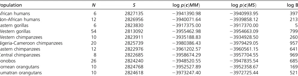
computed the Bayes factors (BF) favoring the more complex model MS (i.e., log BF .0 favors the model with allelic selection) for all populations. It is clear thatMSfits the data considerably better for most of the studied great apes (log BF
.100, Table 1). The only exception is the Eastern gorilla population, for which a lower log BF was obtained (log BF¼5:497, Table 1).
We have also corroborated our BF by inspecting thefit of the predictive distribution of MM and MS with the allele counts (Figure S6, A–K). The allele counts for the polymor-phic states are not symmetrical; generally, one allele is pre-ferred, and thus also the polymorphic states that have it in higher proportions. As expected, we observed thatMSbetter reproduces the skewed distribution of allele counts among great apes.
We further investigated the patterns of allelic selection in great apes by analyzing the posterior distribution of the relative selection coefficients of C, G, and T (sA was set to
0) underMS. A general pattern of allelic selection is observed in great apes: the selection coefficients of C and G are similar (meaning that their posterior distributions largely overlap), but different from the selection coefficient of T, which, in turn, overlaps 0 (approximately equal to the selection coeffi -cient of A) (Figure 2). The only exception is Eastern gorillas, for which the selection coefficients are all only slightly higher than 0 and rather similar (Figure 2). This result corroborates the relatively low BF found for evidence of allelic selection in the Eastern gorilla population.
We further explored this result in order to check if the patterns of GC-bias found among great apes can be associated with gBGC. We correlate the GC-bias per chromosome (by averaging the scaledsCandsG) with the chromosome size and
recombi-nation rate in the non-African human population (Figure S7), for which these data are particularly well characterized (Jensen-Seaman 2004). We found a significant positive correlation between the GC-bias and recombination rate (Spearman’s
r = 0.57,P = 0.006), but a negative correlation with the chromosome length (Spearman’sr = 20.52,P = 0.014).
Although the patterns of selection among great apes are similar qualitatively, they differ quantitatively. For example, Table 1 Evidence of allelic selection among the great ape populations.
Population N S log pðcjMMÞ log pðcjMSÞ log BF
African humans 6 2827135 23941390.98 23940993.95 397
Non-African humans 12 2826956 23940071.64 23939858.12 213
Eastern gorillas 6 2823830 23917375.00 23917370.00 5
Western gorillas 54 2813092 23955462.98 23954663.09 799
Western chimpanzees 10 2823911 23935188.83 23934928.50 260
Nigeria-Cameroon chimpanzees 20 2825739 23980386.43 23979429.05 957
Eastern chimpanzees 12 2822976 23961202.57 23960561.15 641
Central chimpanzees 8 2822685 23958674.29 23957704.55 969
Bonobos 26 2824240 23948520.55 23947835.54 685
Bornean orangutans 10 2824768 23952527.89 23952358.67 169
Sumatran orangutans 10 2824618 23973247.40 23972725.44 521
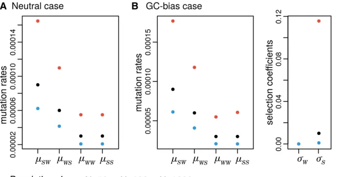
the Central chimpanzees have patterns of GC-bias6.17/4.05 (sC=sG, Table S3 and Figure 2; scaled according to Equation
11), while the closely related population of Western chim-panzees shows less strong patterns (2.21/2.30). Likewise, the GC-bias content in African and non-African human pop-ulations contrasts: 4.47/2.86 and 1.83/1.76, respectively. These results show that the patterns of allelic selection vary greatly among great apes, even among closely related populations.
It has been hypothesized that gBGC is a compensation mechanism for the mutational bias that exists in favor of the weak alleles, A and T (Duret and Galtier 2009; Philippe
et al.2011)—the AT/GC toggling effect. We observed that
mutation rates from strong to weak alleles are more fre-quent (by a factor of 2.80; 3.26 if the stationary frequen-cies are accounted for), while no mutational bias was found between alleles of the same type (1.02; 0.98 if the stationary frequencies are accounted for; Table S3). As the estimated selection coefficients have a clear pattern of GC-bias in most great apes, we can conclude that our
anal-yses are congruent with the expectations of the AT/GC toggling effect.
Furthermore, we compared our method with that of Glémin et al. (2015), by considering only two alleles [the strong (S) and weak (W) alleles] using human allele counts from thefirst human chromosome, divided into 51 regions of 1 million sites (data taken from Glémin et al. 2015). We compared estimates of the gBGC rate coefficient as predicted by our model and that of Glémin et al.(2015) (sS and B,
respectively), and observed that they are negatively corre-lated (Spearman’sr¼ 20:37,p2value = 0.012). Interest-ingly,Bcorrelates significantly with our estimates ofmWS(the
mutation rate of weak to strong alleles;r¼0:50,p2value = 0.001). We have further checked the influence of thefixed sites in our estimates of gBGC, and, as expected, we observed that sS correlates positively with the percentage of
mono-morphic sites (r¼0:36,p2value = 0.012); intriguingly,B
is negatively correlated (r¼ 20:46, p2value = 0.001). Scatter plots of the mentioned correlation tests can all be found in Figure S8.
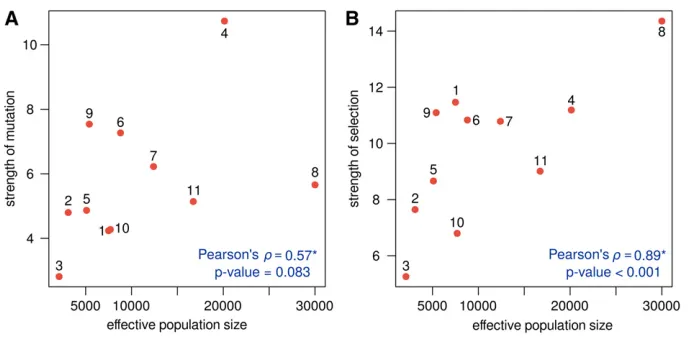
Neand the total rate of mutation and selection in great
apes
It is widely known that the intensity of mutation and selection reflect population demography. To check whether the esti-mated mutation and selection coefficients among great ape populations may be explained by demography, we tested the correlation between the total rate of mutation and selection andNe(obtained from Tenesaet al.(2007); Prado-Martinez
et al.(2013)). Positive correlations between the total
muta-tion and selecmuta-tion rates and the effective populamuta-tion size were obtained (Figure 3): Pearson’s correlation coefficient of 0.57 (P = 0.089) and 0.89 (P , 0.001), respectively. These correlations were obtained using independent contrasts (Felsenstein 1985) accounting for the great apes phylogeny as predicted in Prado-Martinezet al.(2013).
This result shows thatNe plays an important role in
de-termining the intensity of selection. In particular, it becomes clear that the different patterns of GC-bias found among great apes are due, in part, to different demographies. For example, Central chimpanzees have the highest GC-bias among the studied great apes, and they are indeed the pop-ulation that was estimated with the largest Ne (30,000;
Prado-Martinezet al.2013). Eastern gorillas showed the op-posite pattern; this population had no evidence of GC-bias (with very homogeneous selection coefficients) and congru-ently Prado-Martinezet al.(2013) estimated itsNe as only
2000—the lowest of the studied populations.
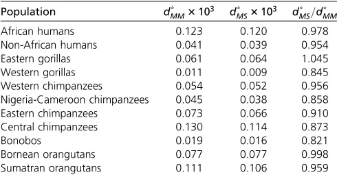
Comparing the expected number of substitutions in great apes
We calculated the expected number of substitutions under
MM and MS to evaluate the impact of allelic selection (in particular, GC-bias) in the evolutionary process. With Equa-tion 6, we calculatedd*
MM andd*MS using the posterior
esti-mates of the respective model parameters. We observe that, for most great ape populations, the expected number of sub-stitutions is lower when allelic selection is accounted for (Ta-ble 2); Eastern gorillas are an exception, and the opposite pattern was observed. We also calculated the ratio between
the expected number of substitutions in both models (i.e.,
d*
MS=d*MM), and we obtained minor (99.8% in Bornean
orang-utans) to major (82.1% in bonobos) deviations; the average difference is27.3% (Table 2). These results suggest that not accounting for GC-bias may distort the reconstructed evolu-tionary process by overestimating the expected number of substitutions.
We complement this result by comparing the posterior distribution of the mutations rates inMMandMS. Because we wanted to identify the mutational types that may be esti-mated differently between these models, we calculated the relative difference between the mutation rate from alleleaito
alleleajusing the following ratio:raiaj¼m MS aiaj=m
MM
aiaj. Ifraiaj.1
for a certain mutation rate aiaj, then this mutation rate is
being underestimated in MM when compared with MS
(and vice versa if raiaj,1); if raiaj1 the mutation rates
are equally estimated in both models.
We observed a systematic bias among great apes. While weak-to-weak and strong-to-strong mutation rates are gen-erally nondeferentially estimated in both models (most of theirroverlap 1, Figure 4) the strong-to-weak and weak-to-strong mutation rates are generally biased inMM. In par-ticular, we obtained that weak-to-strong mutation rates are augmented, while mutations rates from strong-to-weak al-leles are deprecated (Figure 4), which suggests that not ac-counting for GC-bias may bias the estimation of mutation rates. Eastern gorillas behave differently by not showing sig-nificant differences between the estimated mutations rates (allraiajoverlap 1, Figure 4).
Discussion
coefficients) from population data. This work accomplishes tasks set by Schrempf and Hobolth (2017), who observed derivations from neutrality without having a model in place to enlighten the causes.
Variable patterns of gBGC among great apes
A genome-wide application to the great apes provides impor-tant insight into the strength and magnitude of GC-bias patterns and also the impact of gBGC in the evolutionary process. To our knowledge, this is the first work giving a population perspective of the patterns of GC-bias in nonhu-man populations.
Here, we focus on GC-bias because it is a genome-wide effect. Mathematically speaking, it is difficult to disentangle gBGC from directional selection: they may have different biological explanations, but represent the exact same process modeling-wise (i.e., one allele is preferred over the others). Therefore, existing signatures of directional selection are most likely canceling out, when several site-histories (2.8 million sites in our case) are summarized to perform inferences.
In agreement with previous studies in mammals and hu-mans (Spenceret al.2006; Capraet al.2013; Lartillot 2013; Lachance and Tishkoff 2014; Gléminet al.2015), we found that gBGC is weak on average. Indeed, among great apes, the effect of GC-bias is 2.7561.27 (value obtained by averaging scaledsCandsG), consistent with the nearly neutral scenario
(Ohta and Gillespie 1996; Vogl and Bergman 2015). Other studies provided estimates of the scaled conversion coeffi -cient in coding regions: Lynch (2010) estimated 4Nes as
0.82 in humans and Lartillot (2013) adopted a phylogenetic approach that predicted scaled conversion coefficients,1 in all apes. Our estimates are comparatively higher; however, ours methods and those of Lynch (2010) and Lartillot (2013) have different underlying assumptions. In particular, our method employs the Moran model, which has a rate of ge-netic drift twice as fast as the Wright-Fisher model. There-fore, we expect to estimate selection coefficients that are twice as high as those in the studies cited.
We found no quantitative agreement between our esti-mates of the gBGC rate coefficient and those derived from the method of Gléminet al.(2015). In addition, we found that our model attributes to mutation what Gléminet al.(2015) attributes to gBGC. This might be a consequence the use of monomorphic sites in our method. Indeed, unlike those of Glémin et al.(2015), our estimates of gBGC correlate posi-tively with the percentage offixed sizes. In general, the gBGC rate coefficient should promote greaterfixation by boosting the purging of polymorphic sites (at least for low mutation rates, as those observed in humans). On the other hand, Glémin et al.(2015) also considered a varying GC-content, which may explain why their estimates of gBGC do not cor-relate with the percentage offixed sites. We have preliminary evidence showing that monomorphic sites can significantly impact estimates of population parameters. Nevertheless, a more comprehensive model accounting for bothfixed states and variable GC-content would be necessary to disentangle their relative contribution to explaining allele counts.
The patterns of GC-bias we found in great apes are in concordance with the well-known process of gBGC. As expected, we observed that the larger the recombination rate or the lower the chromosome length, the higher the GC-effect. Evidently, recombination promotes gBGC; however, a nega-tive association between gBGC and chromosome size is expected [in most organisms, small chromosomes undergo more recombination per unit of physical distance than large chromosomes (Kaback et al. 1989)]. We performed these analyses in non-African humans, for which these data are available; however, we are confident that the patterns of GC-bias found in great apes are due to gBGC.
It has been hypothesized that GC-bias is a compensation mechanism for the mutational bias that exists in favor of the weak alleles, A and T (Duret and Galtier 2009; Galtieret al.
2009; Philippeet al.2011). Congruent with this expectation, we observed that mutation rates from strong to weak alleles are higher, but rather similar between alleles of the same type. Interestingly, as we have demonstrated, this symmetric manner by which mutations and selection act in great apes leads the number of substitutions to decrease on average. This suggests that AT/GC toggling may increase population variability by promoting more polymorphic sites; however, further studies would be necessary to clarify this prediction.
Intensity of gBGC and demography in great apes
Gléminet al.(2015) hypothesized that differences in GC-bias intensity among human populations were due to the effects of demography. We also advance that demography regulates the intensity of gBGC in great apes. We obtained a positive correla-tion between the total rate of seleccorrela-tion andNein great apes. An
important conclusion of our study is that patterns of gBGC can change rapidly due to demography, even among closely related populations. In fact, most of the studied populations are known to have diverged,0.5 MYA (Prado-Martinezet al.2013).
Here, we showed that GC-bias determines the genome-wide base composition of genomes in a factor proportional to Table 2 Expected number of substitutions per unit of time
Population d*
MM3103 dMS* 3103 d*MS=d*MM
African humans 0.123 0.120 0.978
Non-African humans 0.041 0.039 0.954
Eastern gorillas 0.061 0.064 1.045
Western gorillas 0.011 0.009 0.845
Western chimpanzees 0.054 0.052 0.956
Nigeria-Cameroon chimpanzees 0.045 0.038 0.858
Eastern chimpanzees 0.073 0.066 0.910
Central chimpanzees 0.130 0.114 0.873
Bonobos 0.019 0.016 0.821
Bornean orangutans 0.077 0.077 0.998
Sumatran orangutans 0.111 0.106 0.959
The expected number of substitutions for the four-variate Moran model with boundary mutationsd*
MMand allelic selectiondMS* were calculated based on the
posterior distributions of the model parameters and Equation 6. The relative differ-ence between the average number of events between the two modelsðd*
MS=dMM* Þ
ð1þsC=GÞN21 [or ð1þsÞNe21 in the true dynamic].
There-fore, by either changingNe ors, we are able to change the
AT/GC composition of genomes. Because we were able to correlateNewith the intensity of allelic selection (Pearson’s r = 0.89), we are convinced that demography plays a major role determining the base composition of great ape genomes. Studies using life history traits (i.e., body size) in mammals (Romiguieret al.2010) and ancestral reconstructions of the effective population size in birds (Weber et al. 2014) also advocated for correlations between Ne and GC-content
[al-though not as strong as that found here;r0:3020:55 in Weberet al.(2014)].
In contrast, Galtieret al.(2018) did notfind this correla-tion in a data set covering 31 species of distinct metazoa phyla (including vertebrates, insects, molluscs, crustaceans, echinoderms, tunicates, annelids, nematodes, nemertians, and cnidarians). This is most likely happening because as-pects of the recombination landscape, such as genome-wide recombination rate, length of gene conversion tracts, and repair biases, may also affect the intensity of gBGC (Duret and Galtier 2009; Lesecqueet al.2014; Galtieret al.2018). As the recombination landscape varies significantly across
species, but not so much across closely related populations (e.g., the karyotype is very conserved among great apes, with humans having 46 diploid chromosomes whereas other great apes having 48), we expected stronger correlations between the intensity of gBGC and demography.
Knowing to what extent variations inNeorsdetermine the
base composition of genomes will require further study. In particular, determiningsexperimentally in different popula-tions/species would help assess the real impact of gBGC. If we assume thatsvaries slightly among closely related pop-ulations/species, then we might attribute different intensi-ties of GC-bias almost solely to demographic effects, which simplifies the task of accommodating gBGC in population models.
gBGC calls for caution in molecular and phylogenetic analyses
The effects of gBGC in molecular analysis have been described extensively in the literature [reviewed in Romiguier and Roux (2017)]. We complement these results by showing how GC-bias affects the base composition of genomes, and how the mutation rates and genetic distances may be biased if Figure 4Relative difference in the mutation rates estimated un-der the neutral and non-neutral Moran model.raiaj represents the
ratio between the mutation from alleleai to alleleajin the model with allelic selection and the model with boundary mutations: raiaj¼m
MS aiaj=m
MM
aiaj. The 12
GC-bias is not properly accounted for. In particular, we ob-served that mutation rates from weak-to-strong and strong-to-weak alleles are systematically over and underestimated, respectively.
The idea that gBGC may distort the reconstructed evolu-tionary process comes mainly from phylogenetic studies. For example, it is hypothesized that gBGC may promote substi-tution saturation (Romiguier and Roux 2017). We have shown that the number of substitutions may be significantly overestimated if we do not account for GC-bias, meaning that gBGC may indeed promote branch saturation. Based on this and other gBGC-related complications [e.g., GC-bias pro-motes incomplete lineage sorting (Hobolth et al. 2011)], some authors advocate that only GC-poor markers should be used for phylogenetic analysis (McCormacket al.2012; Romiguier et al. 2013). Contradicting this approach, our results show that we may gain more inferential power if GC-bias is accounted for when estimating evolutionary distances.
Here, we have not performed phylogenetic inference, but previous applications of the Moran model to phylogenetic problems (i.e., PoMo) (De Maioet al.2015; Schrempfet al.
2016) show that it can be done. Therefore, a necessary future work would be to test the effect of allelic selection (or, more specifically, GC-bias) in phylogeny reconstruction; in partic-ular, it would be of major interest to determine how much of its signal can account for the increase in accuracy of tree estimation.
Recently, a nucleotide substitution process that accounts for gBGC was proposed by Lartillot (2013). In this latter model, a scaled conversion coefficient is used to correct sub-stitution rates in a manner similar to that used here to calcu-late the expected number of substitutions for the Moran distance (i.e., assessing the relativefixation probabilities un-der GC-bias, File S3). Therefore, these models should per-form similarly, with the exception that PoMo should be able to disentangle the contribution of selection and mutation to the observed diversity, as it additionally accounts for poly-morphic sites.
Conclusions
Despite widespread evidence of gBGC in several taxa, several questions remain open regarding the role of gBGC in de-termining the base composition of genomes. In this work, we provide a mechanistic model and theoretical results that allow quantification of patterns of gBGC in nonhuman closely related populations, providing a new layer of understanding of the tempo and mode of gBGC evolution in vertebrate genomes.
In addition, our multivariate Moran model with allelic selection makes a significant contribution to the endeavor of estimating population parameters from multi-individual population-scale data. Importantly, our analysis showed that gBGC may significantly distort estimates of population pa-rameters and genetic distances, highlighting that gBGC-aware models should be used when employing molecular
phyloge-netics and population gephyloge-netics analyses. We stress that, although our application to great apes show evidence of GC-bias, our framework can be employed more generally to estimate patterns of nucleotide usage and associated mech-anisms of evolution.
Acknowledgments
We thank Dominik Schrempf, Claus Vogl, and Sylvain Glémin for helpful discussions, and the three anonymous reviewers for comments improving the manuscript. This work was funded by the Vienna Science and Technology Fund (WWTF) through project MA16-061. G.J.S. received funding from the European Research Council under the Eu-ropean Unions Horizon 2020 research and innovation pro-gram under grant agreement no. 714774.
Literature Cited
Baake, E., and R. Bialowons, 2008 Ancestral processes with selec-tion: branching and Moran models. Banach Center Publications 80: 33–52.https://doi.org/10.4064/bc80-0-2
Burden, C. J., and Y. Tang, 2016 An approximate stationary so-lution for multi-allele neutral diffusion with low mutation rates. Theor. Popul. Biol. 112: 22–32. https://doi.org/10.1016/j.tpb. 2016.07.005
Capra, J. A., M. J. Hubisz, D. Kostka, K. S. Pollard, and A. Siepel, 2013 A model-based analysis of GC-biased gene conversion in the human and chimpanzee genomes. PLoS Genet. 9: e1003684.https://doi.org/10.1371/journal.pgen.1003684
Casillas, S., and A. Barbadilla, 2017 Molecular population genetics. Genetics 205: 1003–1035.https://doi.org/10.1534/genetics.116. 196493
Clément, Y., G. Sarah, Y. Holtz, F. Homa, S. Pointet et al., 2017 Evolutionary forces affecting synonymous variations in plant genomes. PLoS Genet. 13: e1006799. https://doi.org/ 10.1371/journal.pgen.1006799
Corcoran, P., T. I. Gossmann, H. J. Barton, J. Great Tit HapMap Consortium, Slateet al., 2017 Determinants of the efficacy of natural selection on coding and noncoding variability in two passerine species. Genome Biol. Evol. 9: 2987–3007.
De Maio, N., C. Schlötterer, and C. Kosiol, 2013 Linking great apes genome evolution across time scales using polymorphism-aware phylogenetic models. Mol. Biol. Evol. 30: 2249–2262.https:// doi.org/10.1093/molbev/mst131
De Maio, N., D. Schrempf, and C. Kosiol, 2015 PoMo: an allele frequency-based approach for species tree estimation. Syst. Biol. 64: 1018–1031.https://doi.org/10.1093/sysbio/syv048
Duret, L., and N. Galtier, 2009 Biased gene conversion and the evolution of mammalian genomic landscapes. Annu. Rev. Genomics Hum. Genet. 10: 285–311. https://doi.org/10.1146/annurev-genom-082908-150001
Durrett, R., 2008 Probability Models for DNA Sequence Evolution
(Probability and its Applications Series, Vol. 34). Springer, New York.https://doi.org/10.1007/978-0-387-78168-6
Etheridge, A. M., R. C. Griffths, and J. E. Taylor, 2010 A coales-cent dual process in a Moran model with genic selection, and the lambda coalescent limit. Theor. Popul. Biol. 78: 77–92.
https://doi.org/10.1016/j.tpb.2010.05.004
Felsenstein, J., 1985 Phylogenies and the comparative method. Am. Nat. 125: 1–15.https://doi.org/10.1086/284325
the coding sequences of reptiles and vertebrates. Genome Biol. Evol. 7: 240–250.https://doi.org/10.1093/gbe/evu277
Fisher, R. a., 1930 The genetical theory of natural selection. Ge-netics 154: 272.
Galtier, N., L. Duret, S. Glémin, and V. Ranwez, 2009 GC-biased gene conversion promotes thefixation of deleterious amino acid changes in primates. Trends Genet. 25:1–5. (erratum: Trends Genet. 25: 287)
Galtier, N., C. Roux, M. Rousselle, J. Romiguier, E. Figuet et al., 2018 Codon usage bias in animals: disentangling the effects of natural selection, effective population size, and GC-biased gene conversion. Mol. Biol. Evol. 35: 1092–1103.https://doi.org/ 10.1093/molbev/msy015
Glémin, S., P. F. Arndt, P. W. Messer, D. Petrov, N. Galtieret al., 2015 Quantification of GC-biased gene conversion in the hu-man genome. Genome Res. 25: 1215–1228. https://doi.org/ 10.1101/gr.185488.114
Goulet, V., C. Dutang, M. Maechler, D. Firth, M. Shapira et al., 2017 expm:matrixexponential, log,’etc’. R package version 0.999–2.
Hastings, W. K., 1970 Monte Carlo sampling methods using Mar-kov chains and their applications. Biometrika 57: 97–109.
https://doi.org/10.1093/biomet/57.1.97
Hobolth, A., J. Y. Dutheil, J. Hawks, M. H. Schierup, and T. Mailund, 2011 Incomplete lineage sorting patterns among human, chim-panzee, and orangutan suggest recent orangutan speciation and widespread selection. Genome Res. 21: 349–356. https:// doi.org/10.1101/gr.114751.110
Jensen-Seaman, M. I., 2004 Comparative recombination rates in the rat, mouse, and human genomes. Genome Res. 14: 528– 538.https://doi.org/10.1101/gr.1970304
Kaback, D. B., H. Y. Steensma, and P. de Jonge, 1989 Enhanced meiotic recombination on the smallest chromosome of Saccha-romyces cerevisiae. Proc. Natl. Acad. Sci. USA 86: 3694–3698.
https://doi.org/10.1073/pnas.86.10.3694
Katzman, S., J. A. Capra, D. Haussler, and K. S. Pollard, 2011 Ongoing GC-biased evolution is widespread in the hu-man genome and enriched near recombination hot spots. Ge-nome Biol. Evol. 3: 614–626. https://doi.org/10.1093/gbe/ evr058
Kimura, M., 1964 Diffusion models in population genetics. J. Appl. Probab. 1: 177–232.https://doi.org/10.2307/3211856
Kluth, S., and E. Baake, 2013 The Moran model with selection:
fixation probabilities, ancestral lines, and an alternative particle representation. Theor. Popul. Biol. 90: 104–112. https:// doi.org/10.1016/j.tpb.2013.09.009
Lachance, J., and S. A. Tishkoff, 2014 Biased gene conversion skews allele frequencies in human populations, increasing the disease burden of recessive alleles. Am. J. Hum. Genet. 95: 408– 420.https://doi.org/10.1016/j.ajhg.2014.09.008
Lartillot, N., 2013 Phylogenetic patterns of GC-biased gene con-version in placental mammals and the evolutionary dynamics of recombination landscapes. Mol. Biol. Evol. 30: 489–502.https:// doi.org/10.1093/molbev/mss239
Lesecque, Y., D. Mouchiroud, and L. Duret, 2013 GC-biased gene conversion in yeast is specifically associated with crossovers: molecular mechanisms and evolutionary significance. Mol. Biol. Evol. 30: 1409–1419.https://doi.org/10.1093/molbev/mst056
Lesecque, Y., S. Glémin, N. Lartillot, D. Mouchiroud, and L. Duret, 2014 The red queen model of recombination hotspots evolu-tion in the light of archaic and modern human genomes. PLoS Genet. 10: e1004790. https://doi.org/10.1371/journal.pgen. 1004790
Liu, H., J. Huang, X. Sun, J. Li, Y. Huet al., 2018 Tetrad analysis in plants and fungi finds large differences in gene conversion rates but no GC bias. Nat. Ecol. Evol. 2: 164–173. https:// doi.org/10.1038/s41559-017-0372-7
Lynch, M., 2010 Rate, molecular spectrum, and consequences of human mutation. Proc. Natl. Acad. Sci. USA 107: 961–968.
https://doi.org/10.1073/pnas.0912629107
Lynch, M., M. S. Ackerman, J.-F. Gout, H. Long, W. Sunget al., 2016 Genetic drift, selection and the evolution of the mutation rate. Nat. Rev. Genet. 17: 704–714. https://doi.org/10.1038/ nrg.2016.104
Marais, G., 2003 Biased gene conversion: implications for genome and sex evolution. Trends Genet. 19: 330–338.https://doi.org/ 10.1016/S0168-9525(03)00116-1
Martin, A. D., K. M. Quinn, and J. H. Park, 2011 MCMCpack: Markov chain Monte Carlo in R. J. Stat. Softw. 42: 22.
https://doi.org/10.18637/jss.v042.i09
McCormack, J. E., B. C. Faircloth, N. G. Crawford, P. A. Gowaty, R. T. Brumfield et al., 2012 Ultraconserved elements are novel phylogenomic markers that resolve placental mammal phylogeny when combined with species-tree analysis. Ge-nome Res. 22: 746–754.https://doi.org/10.1101/gr.125864. 111
Moran, P., 1958 Random processes in genetics. Math. Proc. Camb. Philos. Soc. 54: 60.https://doi.org/10.1017/S0305004100033193
Muyle, A., L. Serres-Giardi, A. Ressayre, J. Escobar, and S. Glémin, 2011 GC-biased gene conversion and selection affect GC con-tent in the Oryza genus (rice). Mol. Biol. Evol. 28: 2695–2706.
https://doi.org/10.1093/molbev/msr104
Nagylaki, T., 1983 Evolution of a finite population under gene conversion. Proc. Natl. Acad. Sci. USA 80: 6278–6281.https:// doi.org/10.1073/pnas.80.20.6278
Ohta, T., and J. Gillespie, 1996 Development of neutral and nearly neutral theories. Theor. Popul. Biol. 49: 128–142.https:// doi.org/10.1006/tpbi.1996.0007
Pessia, E., A. Popa, S. Mousset, C. Rezvoy, L. Duret et al., 2012 Evidence for widespread GC-biased gene conversion in eukaryotes. Genome Biol. Evol. 4: 675–682. https://doi.org/ 10.1093/gbe/evs052
Philippe, H., H. Brinkmann, D. V. Lavrov, D. T. J. Littlewood, M. Manuelet al., 2011 Resolving difficult phylogenetic questions: why more sequences are not enough. PLoS Biol. 9: e1000602.
https://doi.org/10.1371/journal.pbio.1000602
Phillips, M. J., F. Delsuc, and D. Penny, 2004 Genome-scale phy-logeny and the detection of systematic biases. Mol. Biol. Evol. 21: 1455–1458.https://doi.org/10.1093/molbev/msh137
Pouyet, F., S. Aeschbacher, A. Thiéry, and L. Excoffier, 2018 Background selection and biased gene conversion affect more than 95% of the human genome and bias demographic inferences. eLife 7: pii: e36317.https://doi.org/10.7554/eLife. 36317
Prado-Martinez, J., P. H. Sudmant, J. M. Kidd, H. Li, J. L. Kelley
et al., 2013 Great ape genetic diversity and population history. Nature 499: 471–475. https://doi.org/10.1038/ nature12228
R Core Team, 2015 R: A Language and Environment for Statistical Computing. R Foundation for Statistical Computing, Vienna. Roberts, G. O., A. Gelman, and W. R. Gilks, 1997 Weak
conver-gence and optimal scaling of random walk Metropolis algo-rithms. Ann. Appl. Probab. 7: 110–120.
Romiguier, J., and C. Roux, 2017 Analytical biases associated with GC-content in molecular evolution. Front. Genet. 8: 16.https:// doi.org/10.3389/fgene.2017.00016
Romiguier, J., V. Ranwez, E. J. P. Douzery, and N. Galtier, 2010 Contrasting GC-content dynamics across 33 mammalian genomes: relationship with life-history traits and chromosome sizes. Genome Res. 20: 1001–1009. https://doi.org/10.1101/ gr.104372.109
mammals. Mol. Biol. Evol. 30: 2134–2144. https://doi.org/ 10.1093/molbev/mst116
Schrempf, D., and A. Hobolth, 2017 An alternative derivation of the stationary distribution of the multivariate neutral WrightFisher model for low mutation rates with a view to mutation rate estimation from site frequency data. Theor. Popul. Biol. 114: 88–94.https://doi.org/10.1016/j.tpb.2016. 12.001
Schrempf, D., B. Q. Minh, N. De Maio, A. von Haeseler, and C. Kosiol, 2016 Reversible polymorphism-aware phylogenetic models and their application to tree inference. J. Theor. Biol. 407: 362–370.https://doi.org/10.1016/j.jtbi.2016.07.042
Serres-Giardi, L., K. Belkhir, J. David, and S. Glémin, 2012 Patterns and evolution of nucleotide landscapes in seed plants. Plant Cell 24: 1379–1397. https://doi.org/10.1105/ tpc.111.093674
Smeds, L., C. F. Mugal, A. Qvarnström, and H. Ellegren, 2016 High-resolution mapping of crossover and non-crossover recombination events by whole-genome Re-sequencing of an avian pedigree. PLoS Genet. 12: e1006044. https://doi.org/ 10.1371/journal.pgen.1006044
Spencer, C. C. A., P. Deloukas, S. Hunt, J. Mullikin, S. Myerset al., 2006 The influence of recombination on human genetic
diver-sity. PLoS Genet. 2: e148.https://doi.org/10.1371/journal.pgen. 0020148
Tavaré, S., 1986 Some probabilistic and statistical problems in the analysis of DNA sequences. Lect. Math Life Sci. 17: 57–86. Tenesa, A., P. Navarro, B. J. Hayes, D. L. Duffy, G. M. Clarkeet al.,
2007 Recent human effective population size estimated from linkage disequilibrium. Genome Res. 17: 520–526.https://doi.org/ 10.1101/gr.6023607
Vogl, C., and J. Bergman, 2015 Inference of directional selection and mutation parameters assuming equilibrium. Theor. Popul. Biol. 106: 71–82.https://doi.org/10.1016/j.tpb.2015.10.003
Weber, C. C., B. Boussau, J. Romiguier, E. D. Jarvis, and H. Ellegren, 2014 Evidence for GC-biased gene conversion as a driver of between-lineage differences in avian base composition. Genome Biol. 15: 549.https://doi.org/10.1186/s13059-014-0549-1
Webster, M. T., E. Axelsson, and H. Ellegren, 2006 Strong re-gional biases in nucleotide substitution in the chicken genome. Mol. Biol. Evol. 23: 1203–1216.https://doi.org/10.1093/molbev/ msk008
Wright, S., 1931 Evolution in Mendelian populations. Genetics 16: 97–159.
Appendix A
Virtual Population Size
Consider two populations,AandA9;with different population size,NandM, respectively. We want to mimic the dynamics of populationA, relying on the population parameters of a populationA9of different size (larger or smaller). Both populations have the same number of monomorphic states (equaling the number of allelesK) and so we assume them equally frequent in both populations. The number of polymorphic states differs: there areKðN21Þpolymorphic states in populationA, whileA9 hasKðM21Þ. Because we cannot make polymorphic states equivalent, we assume that the sum of polymorphic states for each pairwise comparison of theKalleles should be equal in both populations. These conditions can be written in the following system of equations
(
pfNaig¼p9fMaig
XN21
n¼1pfnai;ðN2nÞajg¼
XM21
m¼1p9fmai;ðM2mÞajg
: (8)
As we have derived an estimator of the site frequency spectrum, we can write this conditions for the multivariate Moran model with boundary mutations and selection as
paið1þsaiÞ N211
k¼p9aið1þs9Þ
M211 k9
paipajraiaj k
XN21
n¼1ð1þsaiÞ
n21ð
1þsajÞN2n21 N
nðN2nÞ¼p9aip9aj r9aiaj
k9
XM21
m¼1ð1þs9aiÞ
m21ð
1þs9ajÞM2m21 M
mðM2mÞ
8 > > < > >
: :
(9)
This system hasKþKðK21Þ=2 conditions and 2K22þKðK21Þ=2 parameters and therefore cannot be solved. However, we know that the entries ofp are constrained in ½0;1and should sum up to 1 in both populations, therefore we make the additional assumption thatpai¼p9ai. In addition, and by definition, the reference allelea
*
i is considered to evolve neutrally in
both systems, which permits the conclusion that the normalization constantskandk9are equal. Simplifying,
pai¼p9ai
ð1þsaiÞN21¼ ð1þs9aiÞM21
raiajXNn¼211ð1þsaiÞn21ð1þsajÞN2n21 N
nðN2nÞ¼r9aiaj
XM21
m¼1ð1þs9aiÞ
m21ð
1þs9ajÞM2m21 M
mðM2mÞ
: 8
> > > > < > > > > :
(10)
we obtain that the population parameters of populationA9can be expressed in terms of the parameters of populationA
p9ai¼pai
ð1þs9aiÞ ¼ ð1þsaiÞMN2211
r9aiaj¼raiaj
PN21
n¼1ð1þsaiÞ
n21ð
1þsajÞN2n21 N
nðN2nÞ
PM21
m¼1ð1þsaiÞ
N21
M21ðm21Þð1þsajÞ N21
M21ðM2m21Þ M
mðM2mÞ
8 > > > > > > > > < > > > > > > > > :
: (11)
This expression looks tedious, but the neutral caseðsai¼0Þcan be very intuitive. In this scenario, mutation rates of populations AandA9change by a factor that is simply the ratio of two harmonic numbers, each of which determined by the population size of the respective population. Intuitively, ifN.M;thenr9aiaj.raiaj, meaning that, in order to compensate the smaller number
of individuals,M(i.e.stronger effect of genetic drift), mutation rates are augmented in populationA9. Figure 5 depicts the effect of the effective population size on the mutation rates and selection coefficients.
Appendix B
Proof of the Stationary Vector
Letcbe a stationary vector ofQ; withcnaiaj andcibeing the elements of the stationary vector corresponding to the states
occurring only in the boundary states, permitting the monomorphic states to communicate with the polymorphic states, while drift and selection are both acting among the polymorphic states. The detailed balance conditions can be defined and lead to equations for the monomorphic and the polymorphic states. In the boundary states, an alleleaiis eitherfixedðn¼NÞor absent
(n¼0,i.e. ajisfixed), for which we may write
ciqNaiaj/N21¼caiajN21qaiajN21/N cjq0aiaj/1¼c1aiajq1aiaj/0; (12)
while, between the polymorphic states, the general condition is valid
cn
aiajqnaiaj/nþ1¼caiajnþ1qnaiajþ1/n : (13)
Condition (13) can be rewritten in the recursive form
cnþ1
aiaj ¼cnaiaj
qn/nþ1
aiaj qnaiajþ1/n
(14)
and then combined with Equation 12
ciqNaiaj/N21¼cnaiajq n/nþ1
aiaj qnaiajþ1/n
. . .q
N22/N21
aiaj
qN21/N22
aiaj
qNaiaj21/N¼cnaiajqnaiaj/nþ1 Y
N21
r¼nþ1
qraiaj/rþ1
qr/r21
aiaj
: (15)
The product can be further simplified by recognizing that, forr¼N21,qN/N21
aiaj ¼maiaj¼pajraiaj, while forr,N21, the rates
inside the product are just the combined rate of drift and selection [according to expression (2)]. We can now rewrite Equation 14 in order to thecn
aiajelement of the stationary vector ofQ
cn aiaj¼
cipajraiaj qnaiaj/nþ1
ð1þsaj 1þsaiÞ
N2n21 :
(16)
Because c0aiaj ¼cj and q
0/1
aiaj ¼mji¼pairaiaj, we obtain a possible solution for the monomorphic states of the stationary
distribution by makingn¼0 in Equation 16
cj ci¼
paj paið
1þsaj 1þsaiÞ
N21:
(17)
The stationary solution for the polymorphic states can be obtained from Equation 16 by noting that ci¼paisNai21 and
qn/nþ1
aiaj ¼ nðN2nÞ
N ð1þsaiÞ
cn
aiaj ¼paipajraiajð1þsaiÞn21ð1þsajÞN2n21 N
nðN2nÞ : (18)
The stationary distribution obtained here can be related with the stationary vector of the neutral boundary multivariate Moran model. We observe that, whens¼0, we obtain the solution computed by Schrempfet al.(2016) for the multivariate Moran model with drift only
ci¼pai cn
aiaj ¼paipajraiaj N
nðN2nÞ : (19)
Appendix C
Proof of the Expected Number of Moran Events per Unit of Time
To assess the impact of allelic selection in branch length estimation (or the total rate of the process), we computed the expected number of events per unit of time for the multivariate Moran model with selection
dMSðt¼1Þ ¼ 2X
u
cuquu ; (20)
Wherecis the stationary vector andquuthe diagonal elements ofQ. Equation 20 can be solved by observing that a
mono-morphic state can be escaped only by mutation, while a polymono-morphic state can be escaped only by selection and drift
dMS¼X
ai2A
X
j6¼i
cimaiajþ X
aiaj2AC
X
N21
n¼1
cn aiaj
nðN2nÞ
N ð1þsaiþ1þsajÞ: (21)
The stationary vector is known from Equations 17 and 18
dMS¼1
k
X
ai2A
X
j6¼i
ð1þsaiÞ
N21pairaiajpa jþ
1
k
X
aiaj2AC
X
N21
n¼1
pairaiajpaj
h
ð1þsaiÞ nð
1þsajÞ
N2n21þ ð
1þsaiÞ n21ð
1þsajÞ N2ni;
(22)
wherekis the normalization constant defined in Equation 4. Expression (22) can be further simplified by observing that the sum in n results in doubling every ð1þsaiÞ
n21ð
1þsajÞ N2n
element. Therefore, the expected number of events can be simplified to
dMS¼2
k
X
aiaj2AC
XN
n¼1
pairaiajpajð1þsaiÞn21ð1þsajÞN2n: (23)
Appendix D
Proof of the Moran Distance in Number Substitutions
The Moran distancedMSaccounts for several events (mutation, driftnewpage, and selection), and differs from the standard
evolutionary distances because they are calculated in terms of the expected number of substitutionsd*
MS.
d*MS¼dMS3s; (24)
wheresis the probability of a substitution.scan be calculated multiplying the probabilitymof an event being a mutation, by the probabilityhof that mutation gettingfixed in the population
s¼ X
aiaj2AP
sai/aj¼
X
aiaj
mai/aj3hjji ; (25)
Solving mai/aj
The probability of an event being a mutation is simply the ratio between the rate of mutation and the total rate (i.e., the rate of mutation plus the rate of drift and selection). In stationarity, we know that the total raterT¼dMSð1Þis simply the expected
number of events of the Moran model and follows Equation 23. The rate of aai/ajmutation is the rate of escaping the
monomorphic statefNaig, from which we can write
mai/aj¼
ri/j
rT ¼
paipajraiajð1þsaiÞN21
2Paiaj2AC
PN
n¼1paipajraiajð1þsaiÞ n21ð
1þsajÞ
N2n: (26)
We can see thatmai/ajdiffers frommaj/aionly due to the selection coefficient in the numerator.
Solving haijaj
According to Kluth and Baake (2013), thefixation probability of an allele withfitness 1þsis for the Moran model
h¼ ð1þsÞ
N21 PN21
n¼0ð1þsÞn
: (27)
As we are using the multivariate Moran model, we have to extend the denominator of (27) to account for the different possible combinations of two selection coefficients. In particular, we may have
haijaj¼
ð1þsaiÞN PN
n¼1ð1þsaiÞ
nð
1þsajÞN2n and hajjai¼
ð1þsajÞN PN
n¼1ð1þsajÞ
nð
1þsaiÞN2n: (28)
We further redefine the denominators in order to make them equal
haijaj¼
ð1þsaiÞNð1þsajÞ PN
n¼1ð1þsaiÞ
nð
1þsajÞN2nþ1 and hajjai¼
ð1þsajÞNð1þsaiÞ PN
n¼1ð1þsajÞ
nð
1þsaiÞN2nþ1: (29)
Solving s
The probability of aai/ajsubstitution under the multivariate Moran model with boundary mutations and selection can be
computed as
sai/aj¼mai/aj3hajjai¼
paipajraiajð1þsaiÞNð1þsajÞN 23Paiaj2ACPNn¼1paipajra
iajð1þsaiÞ n21ð
1þsajÞN2n3PNn¼1ð1þsajÞnð1þsaiÞN2nþ1: (30)
We see thatsai/aj¼saj/ai, which is an expected consequence of stationarity. We can now generalizesai/ajfor all the
sub-stitution types by using Equation 25
s¼P 1
aiaj2AC
PN
n¼1paipajraiajð1þsaiÞ
n21ð
1þsajÞN2n X
aiaj2AC
paipajraiajð1þsaiÞNð1þsajÞN PN
n¼1ð1þsajÞ
nð
1þsaiÞN2nþ1: (31)
The relationship between the Moran distance in events and substitutions can be defined based on Equation 24,
d*MS¼dMSP 1
aiaj2AC
PN
n¼1paipajraiajð1þsaiÞ n21ð
1þsajÞ N2n
X
aiaj2AC
paipajraiajð1þsaiÞNð1þsajÞN
PN
n¼1ð1þsajÞ nð
1þsaiÞ
N2nþ1: (32)
This quantity can be evaluated for neutral regimes:i.e.s/ð0;0;0;0Þ. We obtain the probability of a substitutions under the neutral Moran model, and it matches the result computed by Schrempfet al.(2016):
d*
MS¼dMS
1