of Quintic Threefolds. (Under the direction of Amassa Fauntleroy).
Quintic threefolds are some of the simplest examples of Calabi-Yau varieties. An interesting relationship, discovered by string theorists, is that every Calabi-Yau vari-ety Y has a mirror Calabi-Yau varivari-ety Y. In fact mirror symmetry is a relationship which relates complex structure moduli space of Y to the complexified K¨ahler moduli of its mirrorY . The purpose of this dissertation is to describe the complex structure moduli space from the point of view of geometric invariant theory (GIT).
by
Chirag M. Lakhani
A dissertation submitted to the Graduate Faculty of North Carolina State University
in partial fullfillment of the requirements for the Degree of
Doctor of Philosophy
Mathematics Raleigh, North Carolina
2010
APPROVED BY:
Dr. Larry Norris Dr. Seth Sullivant
DEDICATION
BIOGRAPHY
ACKNOWLEDGMENTS
I would like to begin by thanking my advisor Dr. Amassa Fauntleroy. I am very grateful for his willingness to take me on as a student as an undergraduate and continuing to be my advisor in graduate school. I am very grateful for his willingness to explain algebraic geometry concepts to me over and over and over again. I am also grateful for the wisdom he has imparted about how to do research in mathematics. I will certainly try to heed your advice about not getting stuck in abstract algebraic geometry wonderland but rather find concrete problems which illuminate the abstraction.
To the other members of my committee Dr. Lada, Dr. Norris, and Dr. Sullivant I would like to thank them for their help. To Dr. Lada, I would like to thank him for my first exposure to homological algebra. Little did I know, at the time, that the time spent learning category would actually be useful. I would also like to thank him for the support to attend a conference in Italy. Hopefully, a future paper on L∞
-deformation theory will show the conference was not in complete vain. To Dr. Norris, I would like thank him for all of the patience and time he has given me as I learned geometry. For willing to spend many semesters helping me learn symplectic geometry as well. To Dr. Sullivant, for his advice and willingness to help even in the short amount of time I have known him. I would also like to thank him for organizing such a great tropical geometry seminar. It was one of the most informative seminar series I have ever participated in during graduate school. I am sure many future graduate students will similarly benefit from his enthusiasm and energy.
mathematics I have had with him at Bruegger’s Bagels, the Carmichael gym track and in the mailroom. I am also very grateful to all of the other faculty members in the math department at NCSU. I will certainly treasure how helpful so many professors have been in the course of my time at NCSU.
To the administrative staff at NCSU I am very thankful for all of your help. I am especially thankful to Denise Seabrooks for making my life as a graduate student much easier. I cannot thank her enough for all of help in the job application process as well as fixing bureaucratic messes I would make with the graduate school. To all of the other graduate students I would like to thank you for being so generous and kind during my years at NCSU. The graduate student in the math department are some of the kindest and helpful people I have meet. I treasure the memories and wonderful discussions (mathematical and non-mathematical) that I have had.
TABLE OF CONTENTS
LIST OF TABLES . . . viii
LIST OF FIGURES . . . ix
Chapter 1 Introduction . . . 1
Chapter 2 Geometry of Quintic Threefolds . . . 4
2.1 Geometry of Hypersurfaces . . . 4
2.1.3 Singularities of Hypersurfaces . . . 5
2.2 Parameter Space of Quintic Threefolds . . . 10
2.3 Calabi-Yau Condition . . . 10
Chapter 3 Geometric Invariant Theory . . . 12
3.1 Reductive Groups . . . 12
3.2 Notions of Quotients . . . 14
3.3 Stability and Semistability for Projective Varieties . . . 17
3.4 Hilbert-Mumford Criterion . . . 20
3.5 Minimal Orbits . . . 22
3.6 Quotient Construction for Quintic Threefolds . . . 24
Chapter 4 Semistable Locus . . . 25
4.1 Hilbert-Mumford Criterion for Hypersurfaces . . . 25
4.2 Combinatorics of Maximal Semistable Families . . . 29
4.3 Unstable Families . . . 47
4.4 Bad Flags . . . 47
4.5 Geometric Interpretation of Maximal Semistable Families . . . 49
4.6 Stable Locus . . . 56
Chapter 5 Minimal Orbits . . . 58
5.1 Degenerations . . . 58
5.2 Luna’s Criterion . . . 62
5.3 First Level of Minimal Orbits . . . 64
5.3.1 Minimal Orbit A . . . 64
5.3.3 Minimal Orbit B . . . 69
5.3.5 Minimal Orbit C . . . 71
5.3.7 Minimal Orbit D . . . 72
5.4 Second Level of Minimal Orbits . . . 74
5.4.1 MO2-I . . . 74
5.4.3 MO2-II . . . 75
5.4.7 MO2-IV . . . 81
5.4.9 MO2-V . . . 82
5.4.11 MO2-V . . . 82
5.4.13 MO2-VII . . . 84
5.4.15 MO2-VIII . . . 85
5.4.17 MO2-IX . . . 86
5.4.19 MO2-X . . . 87
Bibliography . . . 90
Appendix . . . 93
Appendix A Code for Poset Structure . . . 94
LIST OF TABLES
Table 4.1 Strictly Semistable Families SS1 - SS4 . . . 31
Table 4.2 Strictly Semistable Families SS5 - SS7 . . . 36
Table 4.3 Strictly Semistable Families SS1 - SS7 . . . 46
Table 4.4 Destabilizing Flags of SS1-SS7 . . . 48
Table 5.1 Corresponding Degenerations of SS1 - SS7 . . . 59
Table 5.2 First Level of Minimal Orbits MO-A - MO-D . . . 59
LIST OF FIGURES
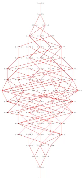
Figure 4.1 Poset structure of quintic monomials . . . 28
Figure 4.2 Poset structure of family SS1 . . . 32
Figure 4.3 Poset structure of family SS2 . . . 33
Figure 4.4 Poset structure of family SS3 . . . 34
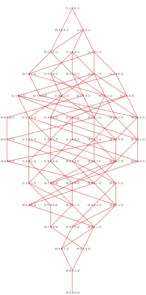
Figure 4.5 Poset structure of family SS4 . . . 35
Figure 4.6 Poset structure of family SS5 I . . . 37
Figure 4.7 Poset structure of family SS5 II. . . 38
Figure 4.8 Poset structure of family SS5 III . . . 39
Figure 4.9 Poset structure of family SS6 I . . . 40
Figure 4.10 Poset structure of family SS6 II. . . 41
Figure 4.11 Poset structure of family SS6 III . . . 42
Figure 4.12 Poset structure of family SS7 I . . . 43
Figure 4.13 Poset structure of family SS7 II. . . 44
Figure 4.14 Poset structure of family SS7 III . . . 45
Figure 5.1 Poset structure of degree 3 monomials . . . 66
Chapter 1
Introduction
Quintic threefolds are a class of projective varieties which occupy a special place in algebraic geometry. They are some of the simplest examples of Calabi-Yau varieties. Calabi-Yau varieties have received a great deal of attention in the last 30 years because they give the right geometric conditions for some superstring compactifications [4]. A surprising geometric relationship found for Calabi-Yau varieties, due to string theory, is a phenomenon called mirror symmetry. Mirror symmetry, in its original form, states that a Calabi-Yau varietyY has a mirror varietyY where the complex structure moduli space of Y is the same as the complexified K¨ahler moduli space of Y. This was explicitly calculated in [5] for the case of quintic threefolds. The purpose of this dissertation is to give an explicit description of the space of complex structure moduli space for Calabi-Yau quintic threefolds using geometric invariant theory (GIT).
polynomial F ∈ C[x0, x1, x2, x3, x4]. In this case, all of the complex structures of
X correspond to deforming the coefficients of the polynomial F [9]. The advantage of this correspondence is that complex structures of quintic threefolds correspond to degree 5 polynomials F ∈ C[x0, x1, x2, x3, x4]. Two polynomials F and F represent
the same complex structure if there is a coordinate transformation which transforms one polynomial into the other. This coordinate transformation on quintic threefolds is given by aSL(5,C) action on the set of degree 5 polynomials. The classification of
complex structures reduces to classifying polynomials F up to a SL(5,C) coordinate
transformation. GIT is a natural tool that can be used to study this problem. GIT is a tool in algebraic geometry used to construct quotient varieties. If a group G acts on an algebraic variety X then, using GIT, one can find the quotient variety X//G. The quotientX//Gis meant to be a variety whose points correspond to unique G-orbits ofX. Unfortunately, this does not always occur. In GIT there can be points
in X//G which represent multiple G-orbits. This means that multiple G-orbits may map to the same point in X//G. Despite this mapping it is still possible to find a unique G-orbit which represents a point in X//G. This unique orbit is called the minimal orbit and its purpose is to give a representative orbit inXwhich corresponds to a point in X//G.
In the preface of [16] the original developer, David Mumford, states that one of his main intentions in developing GIT was so that it can be used to create moduli spaces. Moduli space is a general term that means a space which classifies a class of geometric objects up to some equivalence relation. In the setting of GIT, the variety X would represent the parameter space of all objects which are to be classified. The group G represents the equivalence relations between objects in this parameter space, so the quotient X//G parameterizes objects up to equivalence relation. This approach to constructing moduli spaces has some advantages and disadvantages but it is still a useful method for constructing moduli spaces. This approach has been used to classify certain low degree hypersurfaces in certain Pn [1, 12, 19, 25]. The
in the GIT problem. The quotient variety of the set of smooth hypersurfaces is an open variety. By allowing certain singular hypersurfaces this moduli space can be compactified. One of the goals of this dissertation is to describe which singularities need to be allowed in order to compactify the moduli space of quintic threefolds. The parameter spaces of hypersurfaces have very nice properties which can be used to describe their moduli spaces. A combinatorial method for finding the set of maximal semistable families is explained in Mukai’s book [15] and applied to the case of cubic fourfolds by Laza [12]. This set of maximal semistable families are used to classify the allowable singular hypersurfaces in the moduli space. The combinatorial methods of Mukai and Laza have been used in this dissertation to find the moduli space of quintic threefolds.
Chapter 2
Geometry of Quintic Threefolds
Quintic threefolds are a class of projective varieties which occupy a special place in algebraic geometry. They are some of the simplest examples of Calabi-Yau varieties. Calabi-Yau varieties have received a great deal of attention in the last 30 years because they give the right geometric conditions for some superstring compactifications [4]. A surprising geometric relationship found for Calabi-Yau varieties, due to string theory, is a phenomenon called mirror symmetry. Mirror symmetry, in it’s original form, states that a Calabi-Yau varietyY has a mirror varietyY where the complex structure moduli of Y is the same as the complexified K¨ahler moduli of Y. This was explicitly calculated in [5] for the case of quintic threefolds. The purpose of this dissertation is to give an explicit description of the complex structure moduli for Calabi-Yau quintic threefolds using GIT.
2.1
Geometry of Hypersurfaces
All varieties will be over the complex numbers C.
A quintic threefold is a hypersurfaces in P4 which is defined as the zero locus of a
degree 5 homogeneous polynomial F ∈ C[x0, x1, x2, x3, x4]. Hypersurfaces in Pn are
d hypersurface in Pn if it is the zero locus of a homogeneous degree d polynomial F ∈C[x0, x1, . . . , xn]. The ideal of X is generated by F.
The space Pn is defined as Pn := (Cn+1\[0,0, . . . ,0])/ ∼ where the equivalence
relation is given byx∼yifx= [a0, a1, . . . , an] andy= [λa0, λa1, . . . , λan] forλ∈C∗. Since F ∈C[x0, x1, . . . , xn] is homogeneous it respects the equivalence relation of Pn, so it can be thought of as a hypersurface inCn+1or it descends to a hypersurface inPn. Since hypersurfaces are described by homogeneous polynomials then the geometric characteristics of a hypersurface will be stated in terms of conditions on F.
Remark 2.1.2. We will interchangeably use the fact that a hypersurface X is also given as the zero set of a homogeneous polynomial F. If a homogeneous polynomial F is described as a threefold then it means that the threefold is the zero locus ofF.
2.1.3
Singularities of Hypersurfaces
The study of the different types of singularities which arise in quintic threefolds will be a very important aspect of studying the GIT compactification. One goal will be to classify the types of singularities which will be allowed in the GIT compact-ification. The idea of the GIT compactification is that given the space of smooth quintic threefolds, singular hypersurfaces need to be included in order to compactify the space of quintic threefolds. In the case of cubic threefolds [1] only hypersurfaces with at worst An or D4 isolated singularities need to be included in the GIT
com-pactification. In the case quintic threefolds there will be hypersurfaces which have isolated and non-isolated singularities which must be included in order to compactify the space. This section will give an overview of the singularity terminology which will be used throughout the dissertation.
Given a homogeneous polynomialF, the set of singular points ofF can be defined as the set of points which cause all partial derivatives to vanish. This set of points is defined by the Jacobian ideal ofF.
Definition 2.1.4. Given a homogeneous polynomialF ∈C[x0, x1, . . . , xn] the
singu-lar locus of F is the zero set of the Jacobian ideal hF, ∂F ∂x0,
∂F ∂x1, . . . ,
If a hypersurfaceF of degreedis singular at an isolated point then by a coordinate transformation the singular point can be moved to [1 : 0 : · · · : 0] ∈ Pn. The
homogeneous polynomial can be expanded in terms powers of x0 as follows:
F(x0, x1, . . . , xn) =xd
−1
0 f1(x1, . . . , xn) +. . .+fd(x1, . . . , xn), (2.1) where fi(x1, . . . , xn) is a homogeneous polynomial of degree i in x1, . . . , xn. In order for [1 : 0 : . . . : 0] to be a point in F, the monomial xd
0 can not be included. The
polynomial F is singular at [1 : 0 : . . . : 0] if the the highest power of x0 is xd0−2.
This is the case because the partial derivatives will not vanish at [1 : 0 :. . .: 0] if the power xd−1
0 is present in the polynomial and hence will not be in the Jacobian ideal.
The classification of the singularities, such as the point [1 : 0 : . . . : 0], involve understanding the tangent cone of the singularity. In geometry, the tangent space is the set of all tangent vectors at a point. In general the dimension of the tangent space at a point is the same as the dimension of the space. At a singularity this correspondence breaks down because there are tangent vectors which are not uniquely defined at a singular point. The tangent cone can be thought of as a generalization of the tangent space which provides some information about the singularity.
Definition 2.1.5 (Tangent cone at F). Let [1 : 0 : . . . : 0] be a point of a degree d polynomial F. The tangent cone of [1 : 0 : . . . : 0] at F is the zero locus of the lowest degree polynomial (fi) in the following decomposition. The polynomial F has the decomposition
F :=xd−i
0 fi(x1, . . . , xn) +xd0−i−1fi+1(x1, . . . , xn) +. . .+fd(x1, . . . , xn). (2.2) The degree of the tangent cone is i.
If [1 : 0 :. . .: 0] is non-singular then the tangent cone is the tangent spacef1 ofF.
than or equal to i [2]. Intersection multiplicity is used to count the degeneracy of intersections of two varieties in complimentary dimensions.
Definition 2.1.6(Intersection Multiplicity c.f. [2] p.103). For two projective varieties X,Y ∈Pnwhere dimX + dimY =n, let I(X) andI(Y) be the homogeneous ideals defining X and Y. For a point of intersection p∈X∩Y the intersection multiplicity
of p is
mp(X, Y) :=dimC OPn,p/(I(X) +I(Y))
, (2.3)
wheredimC means dimension as a complex vector space andOPn,p is the structure
sheaf localized at the point p.
This definition is used to generalize the familiar notion that a curve of degree d and curve of degree e intersect inde points.
Theorem 2.1.7 (Bezout’s theorem [2] ch.4). For two curves C1, C2 ∈P2 of degree d
and degree e respectively, if they intersection in finite points then following relation holds,
X
p∈C1∩C2
mp(C1, C2) =de. (2.4)
Theorem 2.1.8 (Generalized Bezout’s Theorem [2] ch.4). For two Cohen-Macaulay projective varieties X, Y ∈ Pn where dim X + dim Y=n and having degree d and
degree e respectively, the following relation holds,
X
p∈X∩X
mp(X, Y) =de. (2.5)
points of intersection of a line with a degree d hypersurface will sum up to d when intersection multiplicity is taken into account.
The geometric interpretation of the tangent cone gives a method for classifying singularities. The first coarse classification of singularities that arise in quintic three-folds is to classify singularties by describing their tangent cones. The higher the degree of the tangent cone the more complicated the singularity. Unfortunately clas-sifying tangent cones is not enough to completely describe the singularities that arise in quintic threefolds. The decomposition (2.2) can also give some finer data about intersection multiplicities. As stated earlier, the zero locus of fi give the set of points whose lines with [1 : 0 : . . . : 0] which intersect F . The iintersection multiplicity of this line with F is least i. The decomposition (2.2) gives a filtration for higher multiplicity intersections with [1 : 0 :. . .: 0]. The set of lines which have intersection multiplicity at least i+ 1 is given by the zero locus of bothfi and fi+1.
Proposition 2.1.9 ( [2] p.110). Given a degree d polynomial F with [1 : 0 : . . . : 0]
as its singular point, degree i tangent cone, and decomposition of the form (2.2), the set of lines whose intersection multiplicity with [1 : 0 : . . .: 0] is at leastr is given by the zero locus of fi =fi+1=. . .=fi+r where i≤r≤d−i−1.
This proposition will be important when classifying singularities of quintic three-folds in chapter 4. The classification of singularities will include characterizing the tangent cone to the singularity as well it’s higher order intersection multiplicities. When restricting to the case of polynomials in P4, a polynomial is of the form
F ∈ C[x0, x1, x2, x3, x4]. The degree of the tangent cone and decomposition (2.2)
for a polynomial F also give information about the maximum multiplicity of the the ideal hx1, x2, x3, x4i which contains F.
Definition 2.1.10. Given the a homogeneous polynomial F with singular point [1 : 0 : 0 : 0 : 0], the singular point is a
1. double point if the degree of the tangent cone is 2 i.e. F ∈ hx1, x2, x3, x4i2,
3. and a quadruple point if the degree of the tangent cone is 4 i.e. F ∈ hx1, x2, x3, x4i4.
The definitions double point, triple point, and quadruple point can be extended to non-isolated singularities. If F has a non-isolated singularity such as a line or plane then, by a change of coordinates, it can be mapped to lines and planes in standard coordinates. We will focus only on lines and planes since they are the singularities which arise in the GIT quotient of quintic threefolds. A line can be represented by coordinates [a : b : 0 : 0 : 0] ∈ P4 the ideal for this line is hx
2, x3, x3i. A plane can
be representated by the coordinates [a : b : c : 0 : 0]∈ P4 the ideal for this plane is
hx3, x4i. Singular lines and planes, similar to the case of points, can be defined using
their ideals.
Definition 2.1.11. Given the a homogeneous polynomial F with singular line [a:b: 0 : 0 : 0], the singular line is a
1. double line if F ∈ hx2, x3, x4i2,
2. triple line if F ∈ hx2, x3, x4i3,
3. and quadruple line if F ∈ hx2, x3, x4i4.
Definition 2.1.12. Given the a homogeneous polynomial F with singular plane [a:b:c: 0 : 0], the singular plane is a
1. double plane if F ∈ hx3, x4i2,
2. triple plane if F ∈ hx3, x4i3,
3. and a quadruple plane if F ∈ hx3, x4i4.
Remark 2.1.13. In algebraic geometry if a hypersurface is contained in an ideal F ∈ hxa1, xa2, . . . , xari
d then it is known that the zero locus of hx
a1, xa2, . . . , xari
d
denoted V(hxa1, xa2, . . . , xari
d) is contained in the zero locus of F denoted V(F) i.e. V(hxa1, xa2, . . . , xari
d)⊆V(F). We will use these notions interchangeably. The state-ment ”X contains the ideal hxa1, xa2, . . . , xari
These singularities will give a complete classification of singularities which arise in the GIT compactification of quintic threefolds.
2.2
Parameter Space of Quintic Threefolds
In P4 there are 9 5
= 126 degree 5 variables. An arbitrary quintic threefoldF can be written in the following form
F(x0, x1, x2, x3, x4) :=
X
i+j+k+l+m=5
aijklmxi0x
j
1x
k
2x
l
3x
m
4 . (2.6)
The 126 coefficients aijklm can be thought as coordinates of a 126 dimensional vector space which represent the polynomialF. As a representation this vector space is denoted Sym5(C5). Since the hypersurfaces are in projective space thenF and λF
represent the same polynomial therefore Sym5(C5) needs to be projectivized.
Definition 2.2.1. The parameter space of quintic threefolds isP(Sym5(C5))
The vector space Sym5(C5) is an SL(5,C)-reprsentation, which comes from the
natural action ofSL(5,C) onP4. The GIT compactification, as discussed in the next
chapter, corresponds to quotienting P(Sym5(C5)) by SL(5,C).
2.3
Calabi-Yau Condition
As stated earlier, quintic threefolds are some of the simplest example of Calabi-Yau varieties. If a Calabi-Calabi-Yau variety is a manifold then there are many equivalent definitions of a Calabi-Yau manifold.
Definition 2.3.1. A smooth and compact K¨ahler manifoldX is Calabi-Yau if it has the following equivalent properties:
3. the holonomy group of X isSU(n),
4. there exists a K¨ahler metric on X with vanishing Ricci curvature.
The various equivalences between these statements have been proven such as in Yau [24]. One of the more difficult equivalences to be proved was (2)⇒(4). This was the conjecture proposed by Calabi and proven by Yau [24]. For the case of quintic threefolds the adjunction formula can be used to show that ωX is trivial.
Proposition 2.3.2 (Adjunction formula [18] p.40). Let X ⊆ Y be a non-singular hypersurface. ThenωX = (ωY⊗OY(X))|X, whereOY(X)is the line bundle associated
to the hypersurface X.
If X is a degree d hypersurface and Y = P4 then ω
Y ∼= OP4(−5) and OY(X) ∼=
OP4(d). By the adjunction formula
ωX = (OP4(−5)⊗ OP4(d))|X = (OP4(d−5))|X. (2.7)
For the quintic threefold ωX = (OP4(0))|X =OX, so X satisfies the condition to
Chapter 3
Geometric Invariant Theory
In this section we will describe the theory of geometric invariant theory. Broadly speaking, given a groupG acting on a variety X, geometric invariant theory gives a method of constructing a quotient variety X//G. The varietyX//G, as the quotient of the parameter space of quintic threefolds, is supposed to parameterize G-orbits of points on X. In the general setting, there are bad orbits which must not be included in the construction of X//G and there may be several orbits which map to same point in X//G. In order to give a precise description of these caveats the notion of semistable, stable and unstable points will be introduced. In this chapter various definitions of quotients, various definitions of stability, and how quotients are formed will all be discussed.
3.1
Reductive Groups
Definition 3.1.1. Alinear algebraic groupGoverCis a closed subgroup ofGL(n,C).
Definition 3.1.2. Areductive linear algebraic group is a linear algebraic group whose radical (connected component of the maximal normal solvable subgroup which con-tains the identity) is diaganolizable.
One of the advantages of using reductive linear algebraic groups is that their repre-sentations are completely reducible. This property was very important in Mumford’s development of GIT.
Definition 3.1.3 (c.f. [11] p.98 ). If G is a linear algebraic group with a rational representation (ρ, V) then the representation is completely reducible if for every G-invariant subspace W ⊆V there exists a G-invariant subspace U where V =W⊕U. Proposition 3.1.4(c.f. [11] p.98). Every rational representation of a reductive linear algebraic group is completely reducible.
Reductive linear algebraic groups also have the nice property that if such a group G acts on a ring A, which is finitely generated over C, then the ring of invariants,
AG, is finitely generated. This is important in GIT because the ring of invariantsAG will be the ring used to construct the quotient space.
Theorem 3.1.5 (Nagata’s Theorem). [ [6] p.41] If G is a reductive linear algebraic group which acts on a ring A then the ring of invariants AG, from this action, is
finitely generated.
Nagata’s Theorem gives a natural way to map an affine varietyX = Spec(A) with a linear reductive group actionGinto a G-invariant space. SinceAG ⊆Aon the level of rings, this inclusion reverses to give
Φ :X →Spec(AG). (3.1)
Since AG is finitely generated by Nagata’s theorem, the quotient Spec(AG) is an
This induced map Φ is a dominant morphism (the image Φ(X) is dense in Spec(AG).
Nagata’s theorem is also important when looking at quotients of projective vari-eties. In the case of a projective variety X = Proj(A) the inclusionAG ⊆A generates a map Φ :X = Proj(A)→ Proj(AG). This map is only a rational map. In order to
get a morphism for this map, we need to restrict to a subset of points onX called the semistable points (Xss) which will map into Proj(AG). This will be explained further
in the next sections.
3.2
Notions of Quotients
For the remainder of this dissertation we will assume all groups are reductive linear algebraic groups unless otherwise specified.
In GIT there are various types of quotients. Following Lakshmibai [11] we will give describe three standard types of quotients: the categorical quotient, good quotient, and geometric quotient. We will also describe the relationships between these different notions of quotients . In the previous section it was shown that some notion of a quotient space can be constructed by taking Spec or Proj of the ring of invariants. In the next sections we will describe precisely how Spec and Proj are related to categorical, good, and geometric quotients.
Definition 3.2.1 (Categorical quotient [11] p.102). Given a group action of G on a variety X, acategorical quotient is a variety Y and aG-invariant morphism
Φ :X →Y (3.2)
X Φ˜ // Φ ? ? ? ? ? ? ?
? Y˜
Y τ ? ?
commutes. Denote the categorical quotient Y := X//G. It is unique up to iso-morphism.
The universal property shows that allG-invariant morphisms must factor through Φ therefore a categorical quotient X//G for a G-action on X is unique. A more restrictive class of categorical quotients are good quotients. In this dissertation we will more concerned with good quotients.
Definition 3.2.2 (Good quotient [11] p.103)). Given a group G acting on a variety X, a good quotient of the G-action of X is a variety Y and a G-invariant morphism Φ :X→Y with the following properties:
1. Φ is surjective;
2. For any open subset U ⊆ Y, Φ−1(U) ⊆ X is open and affine if and only if
U ⊆Y is open and affine;
3. for any open subset U ⊆Y the homomorphism of rings;
Φ∗
:OY(U)→ OX(Φ
−1(U)) (3.3)
is an isomorphism onto O(Φ−1(U))G;
4. if W ⊆X isG-stable and closed then Φ(W) is closed;
5. if W1 and W2 are two disjoint G-stable closed subsets ofX, then
Φ(W1)∩Φ(W2) =∅.
From the definitions it is not obvious that good quotients satisfy the universal mapping property (3.2.1) in the categorical quotient definition. Since good quotients behave well locally it can be shown that they satisfy the universal mapping property. Proposition 3.2.3 (c.f. [11] p.104). A good quotient is a categorical quotient. Remark 3.2.4. In the case of aG-action on an affine varietyX = Spec(A) the quotient X//G = Spec(AG) from (3.1) is a good quotient.
Definition 3.2.5 (Orbit Space). Given a group G acting on a variety X, a variety Y and G-invariant morphism Φ :X →Y is an orbit space if each y∈Y corresponds to a unique G-orbit in X i.e. Φ−1(x) is a G-orbit.
Definition 3.2.6 (Geometric quotient [11] p.105). A good quotient (Y,Φ) which also an orbit space is called a geometric quotient. We will denote the geometric quotient as X/G
A geometric quotient is an ideal type of quotient in GIT. Along with the properties of a good quotient, a geometric quotient parameterizes precisely the G-orbits of X. This is not the case for a good quotient, where it is possible for two different orbits to map to the same point in the good quotient.
Definition 3.2.7. For a G-action on X if x ∈ X then Gx := {gx|g ∈G} is the G-orbit of x. The spaceGx is the closure of Gx in X.
Proposition 3.2.8 (c.f. [11] p. 104). For a G-action on a variety X if (X//G,Φ) is a good quotient then Φ(x1) = Φ(x2) if and only if Gx1∩Gx2 6=∅.
Lemma 3.2.9 (Closed orbit lemma [3, 11]). For a G-action on a variety X each
G-orbit Gx is a smooth variety which is open in its closure. The boundary of the
G-orbit, Gx\Gx, is a union of strictly smaller dimensional G-orbits. The orbits of minimal dimension are closed.
Definition 3.2.10. For a G-action on X, a minimal orbit is a closed G-orbit of smallest dimension in Gx.
If a G-orbit is closed then it is a minimal orbit because there are no other orbits in it’s closure. In this dissertation we will be concerned with finding minimal orbits in the closure of non-closed orbits. The minimal orbit will be considered a degeneration of the larger non-closed orbit.
Definition 3.2.11. Given a G-action on X and a x∈X, a degeneration of Gx is a minimal orbit in Gx
3.3
Stability and Semistability for Projective
Va-rieties
In the case of affine varieties it is easy to describe quotient spaces. The map (3.1) is a morphism of varieties from X to a quotient. If X = Proj(A) is a projective variety then the corresponding quotient
Definition 3.3.1 (Linearization of G-action). Given a G-action on a projective va-riety X, a linearization of the G-action is a representation
ρ:G→GL(V) (3.5)
where X ⊆ P(V) is closed in P(V) and the G-action on X is induced by the
representation given by (3.5).
The extra data that a linearization provides is an embedding of X into some projective space P(V) and the extension of the G-action of X onto this ambient
projective space. In the case of quintic threefolds the linear action is canonically defined. As shown in chapter 2, the space of quintic threefolds is P(Sym5(C5)). The
linearization of SL(5,C)-action on P(Sym5(C5) is naturally defined in this situation.
Definition 3.3.2. Thelinearization of the SL(5,C) action on P(Sym5(C5)) is given
by the 5th symmetric power (Sym5) representation of the standard SL(5,C)
repre-sentation on C5.
Given a linearization, a point x ∈ X ⊆ P(V) can be viewed as an element in
V up to projective equivalence. This correspondence gives a precise definition for semistability.
Definition 3.3.3 (Semistable). Given a G-action on X with a linearization V, a point x∈X is semistable if there is a representative ˆx∈V of x where 0∈/ Gˆxin V. The set of semistable points in X will be denoted Xss.
Definition 3.3.4 (Unstable). Given a G-action on X with a linearization V, a point x ∈ X is unstable if it is not semistable. The set of unstable points in X will be denoted Xus.
for good quotients of projective varieties. They will be precisely the points which are thrown away in order to make (3.4) into a morphism of varieties. To define a geometric quotient the set of semistable points must be further restricted to stable points.
Definition 3.3.5 (Stable). Given a G-action on X with a linearization V, a point x∈X isstable if there is a representative ˆx∈V of x such that:
1. 0 ∈/ Gˆx;
2. the orbit Gˆx is closed;
3. the isotropy group, Gx, of ˆxis finite.
The set of stable points in X will be denoted Xs. Note: Xs ⊆Xss due to condition 1.
Definition 3.3.6 (Strictly semistable). Given a G-action on X with a linearization V, a point x∈X is strictly semistable if it is semistable but not stable.
These definitions give precisely the conditions needed to determine the geometric quotient and good quotient for a G-action on X.
Theorem 3.3.7 (c.f. [11, 17] ). Let there be a G-action on X = Proj(A) with a linearziation X ⊆P(V). The set of semistable points Xss have a good quotient
Φ :Xss→X//G:=Xss//G= Proj(AG). (3.6)
The good quotient X//G is a projective variety and Φ is surjective.
Theorem 3.3.8 (c.f. [11, 17] ). Let there be a G-action on X = Proj(A) with a linearziation X ⊆P(V). The set of stable points Xs have a geometric quotient
Φ :Xs →Xs/G. (3.7)
Remark 3.3.9. It is also important to note that these definitions of stable, semistable, and unstable depend on the choice of linearization. A different choice of linearization may change the set of semistable points. A very interesting connection to varying the choice of linearization and birational transformations of quotients is given in the papers of Thaddeus [22] and Dolgachev-Hu [7]
In the case of projective varieties the geometric quotient Xs/Gis the orbit space which represents all of the ”nice orbits” in the GIT quotient. The good quotient X//G gives a compactification ofXs/G. The boundary X//G\Xs/G correspond to the most degenerate orbits in the GIT quotient.
3.4
Hilbert-Mumford Criterion
Using only the definitions it is, in general, very difficult to determine precisely which points are semistable and stable. One of Mumford’s innovative ideas in GIT was to provide a numerical method for determining which points are semistable and stable. The criterion uses the set of one parameter subgroups (1-PS) of G.
Definition 3.4.1 (One-parameter subgroup (1-PS)). Given a groupG a1-PS λ is a homomorphism
λ:C∗
→G. (3.8)
A 1-PS can be thought of as a function λ(t) where t∈C∗
.
Given a linearizedG-action onXand a pointx∈Xwith representative ˆx∈V, the Hilbert-Mumford criterion gives a method for determining whether x is semistable or stable using the set of 1-PS of G. Given a 1-PS λ the vector space V can be decomposed into weight spaces
V =M i∈Z
Wi (3.9)
ˆ x=X
i
wi. (3.10)
The decomposition of the point ˆx using a 1-PS λ is needed to define Mumford’s numerical function.
Definition 3.4.2 (Mumford’s numerical function). Given a G-action on X with a linearizationV, a point x∈X, and a 1-PSλ,Mumford’s numerical function is
µ(x, λ) = −min{i, wi 6= 0}. (3.11) The vectors wi come from the decomposition (3.10) associated to the 1-PS λ.
A 1-PS λ has a diagonalized action on the vector space V. This decomposes the point ˆx into a sum of weight vectors. The Hilbert-Mumford numerical function’s value on ˆx is the negative of the lowest weight of that point with respect to the diaganolization. The Hilbert-Mumford criterion states that x ∈ X is semistable or stable precisely when x satisfies certain properties of the numerical function.
Theorem 3.4.3 (Hilbert-Mumford criterion [11,16,17]).Given aG-action onX with a linearization V, a point x∈X is
1. semistable if and only if µ(x, λ)≥0 for all 1-PS λ in G; 2. stable if and only if µ(x, λ)>0 for all 1-PS λ in G.
The numerical function must be nonnegative or positive for all 1-PSλ. One way of thinking of a semistable or stable point is that it has some positive and some negative weights since the criterion must be satisfied by allλand its inverseλ−1. One difficulty
of Mumford’s criterion is that the numerical function must be checked for all 1-PS λ of G. There is one property of the numerical function that allows one to restrict the number of 1-PS λ that need to be checked.
Lemma 3.4.4 ( [11]). For a point x∈X and a 1-PS λ
µ(x, λ) = µ(gx, gλg−1) (3.12)
This property is useful if one is concerned with classification of G-orbits rather than just one particular point. One interpretation is that all 1-PSλcan be conjugated togλg−1while still saying in the sameG-orbit. Despite the ability to restrict the class
of 1-PSλ it is still quite cumbersome to calculate the stability or semistability for a point x ∈ X. By taking the negation of the Hilbert-Mumford criterion, the criteria for determining whether a point is unstable or strictly semistable points results from the existence of a 1-PS λ which causes the Hilbert-Mumford criterion to fail.
Proposition 3.4.5. Given a G-action on a variety X with linearization V, a point
x∈X is
1. unstable if and only if there exists a 1-PSλ such that µ(x, λ)<0;
2. strictly semistable if and only it is not unstable and there exists a 1-PS λ such that µ(x, λ) = 0.
In the case of quintic threefolds the existence of such a 1-PSλ can be determined using linear programming which will be explained in the next chapter.
3.5
Minimal Orbits
Proposition (3.4.5) shows that a strictly semistable point x ∈ X has a 1-PS λ where µ(x, λ) = 0. This means that given the weight decomposition (3.10) the point ˆ
x will have all nonnegative weights.
Definition 3.5.1 (Destabilizing 1-PS). Given a G-action onX with linearizationV, a strictly semistable point x∈X has a destabilizing 1-PS λ if µ(x, λ) = 0.
Since the weight decomposition of x, induced by a destabilizing 1-PS λ, has all nonnegative weights then one can take the closure of the λ orbit of x.
Definition 3.5.2 (Degeneration of Strictly Semistable Point). Given a strictly semistable point x with destabilizing 1-PSλ the degeneration of xis
λx:= lim
From previous sections it was discussed that closure of orbits map to the same point in a good quotient. If it is known that a point x ∈ X is strictly semistable and λ is its destabilizing 1-PS then the point x and λx will map to the same point in the geometric quotient. For the GIT compactification, the minimal orbits give unique representative of points in the boundary X//G\Xs/G. Minimal orbits can be systematically found using degenerations. In the weight space decomposition of a strictly semistable point x the degeneration λx causes all weight vectors which have non-zero weights to vanish. When determining minimal orbits this significantly reduces the complexity of the problem since only the weight vectors which have weight 0 need to be analyzed.
Proposition 3.5.3. Given a strictly semistable point x∈X with destabilizing 1-PS
λ, the degeneration λx is invariant under λ.
Proof. Let x be a strictly semistable point with destabilizing 1-PS λ. Using the decomposition (3.10) the action of λ on ˆx is of the form
λ(t)ˆx=X i∈Z
tiw
i. (3.14)
Since µ(x, λ) = 0 then all i ≥0. Then in λˆx the ti go to zero unless i= 0. The only weight vectors of λˆx which are still left correspond to vectors with weight 0. Therefore, they are invariant underλ.
3.6
Quotient Construction for Quintic Threefolds
As stated in Chapter 2, the parameter space for quintic threefolds is the space
P(Sym5(C5)). The natural action of SL(5,C) on the coordinates of P4 induces a
representation on the linearzation V = Sym5(C5). The GIT compactification of
in-terest in this dissertation is the quotientP(Sym5(C5))//SL(5,C). To give an explicit
description of the quotientP(Sym5(C5))//SL(5,C) the problem of determining which
Chapter 4
Semistable Locus
This section will describe the semistable locus of the GIT compactification. In particular, using the Hilbert-Mumford numerical criterion, we will explicitly descibe the strictly semistable points of the GIT compactification. The advantage of using the Hilbert-Mumford criterion is that a strictly semistable or unstable point is detected by showing the existence a 1-PS which causes the criterion to fail. By restricting to a certain family of 1-PS one can use the Hilbert-Mumford criterion to find the maximal strictly semistable families of hypersurfaces. One can then study the singularities of these families using the principle of bad flags. These results can, in turn, be used to give a partial description of hypersurfaces in the stable locus.
4.1
Hilbert-Mumford Criterion for Hypersurfaces
Given the linearization V =Sym5(C5), a point v ∈V represents a quintic
hyper-surface. A modification of the Hilbert-Mumford criterion explicitely determines the set of semistable points.
Proposition 4.1.1. Given a G-action on a variety X with linearization V, a point
v ∈V is
2. and strictly semistable if and only it is not unstable and there exists a 1-PS λ
such that µ(v, λ) = 0.
This modification of the Hilbert-Mumford criterion shows that determining whether v is semistable or unstable amounts to finding a 1-PS which satisfies the right condi-tions on the numerical function.
Definition 4.1.2. A destabilizing 1-PS λ : C∗
→ SL(5,C) of a strictly semistable
(unstable) point v, is a 1-PS such that µ(v, λ) = 0 (µ(v, λ)<0). The G-equivariant property of the numerical function µ, namely,
µ(gv, gλg−1) =µ(v, λ), (4.1)
can be used to restrict the class of 1-PS.
If the standard torus T ⊆ SL(5,C) is fixed then a 1-PS λ : C∗
→ T acts on xi
0x
j
1xk2xl3xm4 by the following action:
λ(t)xi 0x j 1x k 2x l 3x m
4 =t
ai+bj+ck+dl+emxi
0x j 1x k 2x l 3x m
4 . (4.2)
Every such λ can be represented by a vector ha, b, c, d, ei, which are the weights of the C∗
-action on each degree 1 monomial. One simplyfying assumption that can be made is that every 1-PS λ can be conjugated to a standard 1-PS.
Proposition 4.1.3. Given a 1-PS λ : C∗ →
SL(5,C) it can be conjugated (gλg−1)
to a 1-PS λ:C∗
→T represented by the vector ha, b, c, d, ei where a ≥b≥c≥d≥e
and a+b+c+d+e= 0. This class of 1-PS will be called a normalized 1-PS.
Since we are interested in finding strictly semistable hypersurfaces, up to aSL(5,C)
coordinate transformation, the G-equivariance of the Hilbert-Mumford numerical function allows us to restrict to a normalized 1-PS given by the proposition 4.1.3. By restricting to normalized 1-PS there is an ordering that can be put on the mono-mials which determine a poset structure on the set of quintic monomono-mials. We will represent a monomial xi
0x
j
Definition 4.1.4. For a monomial [i, j, k, l, m] if there is a normalized 1-PS λ = ha, b, c, d, ei which acts on the monomial via the diagonal action shown above then, by the definition of the numerical function,
µ([i, j, k, l, m],ha, b, c, d, ei) =ia+jb+kc+ld+me (4.3) i.e. the dot product of the vectors.
Definition 4.1.5. The set of monomials [i, j, k, l, m] has a partial order given by [i0, i1, i2, i3, i4]≥[j0, j1, j2, j3, j4] if
µ([i0, i1, i2, i3, i4], λ)≥µ([j0, j1, j2, j3, j4], λ) (4.4)
for all normalized 1-PS λ of Prop. 4.1.3.
The following lemma gives a numerical method for determining the poset structure on monomials.
Lemma 4.1.6(c.f. [15] p.225). For two monomials[i0, i1, i2, i3, i4]and[j0, j1, j2, j3, j4]
[i0, i1, i2, i3, i4]≥[j0, j1, j2, j3, j4]⇐⇒
i0 ≥j0
i0 +i1 ≥j0+j1
i0 +i1+i2 ≥j0+j1+j2
i0 +i1+i2+i3 ≥j0+j1+j2+j3
4.2
Combinatorics of Maximal Semistable
Fami-lies
In this section we will show how the poset structure can be used to determine the set of maximal semistable families. The restriction to normalized 1-PS from Prop 4.1.3 allows us to use linear programming to find these maximal semistable families. We can precisely define these maximal stable families using terminology from posets. Definition 4.2.1 (c.f. [20] section 3.1). Given a poset P with a partial ordering ≥, a subset I ⊆P is called an ideal if ∀x, y ∈P where x∈I and x≥y, then y∈I. Definition 4.2.2. For a monomial [i, j, k, l, m] define the set
I([i, j, k, l, m]) := {[a, b, c, d, e]|[i, j, k, l, m]≥[a, b, c, d, e]}. (4.5) From the definition I([i, j, k, l, m]) is an ideal of the poset.
The set I([i, j, k, l, m]) represent all vectors below [i, j, k, l, m] in the poset. The set of polynomials associated to I([i, j, k, l, m]) is denoted P(I([i, j, k, l, m])).
Definition 4.2.3. The setP(I([i, j, k, l, m])) represents all polynomials of the form X
a+b+c+d+e=5
rabcdexa0xb1xc2xd3xe4 (4.6)
where [a, b, c, d, e]∈I([i, j, k, l, m]).
Lemma 4.2.4. For a polynomial F ∈P(I([i, j, k, l, m])) and normalized 1-PS λ
µ(F, λ) = µ([i, j, k, l, m], λ). (4.7)
Definition 4.2.5. Given a normalized 1-PSλ let
M(λ) := {[i, j, k, l, m]|µ([i, j, k, l, m], λ)≤0}. (4.8) A maximal semistable family is precisely a set M(λ) where there exists no λ where M(λ)⊆ M(λ).
Due to the poset structure, there is a set of maximal monomials which define each set M(λ). This property is useful because the maximal monomials can be used to describe the general form of the equation for some familyM(λ).
Lemma 4.2.6. For a fixed 1-PS λ, the family M(λ) has a set of monomials
[i1
0, i11, i12, i13, i41], [i20, i21, i22, i23, i24], . . . [ir0, i1r, ir2, ir3, ir4] where
M(λ) =I([i1 0, i
1 1, i
1 2, i
1 3, i
1
4])∪I([i 2 0, i
2 1, i
2 2, i
2 3, i
2
4]). . .∪I([i
r
0, i
r
1, i
r
2, i
r
3, i
r
4]). (4.9)
The maximal monomials are the set of monomials [i, j, k, l, m] ∈ M(λ) where there are no other monomials[a, b, c, d, e]such that I([i, j, k, l, m])⊆I([a, b, c, d, e])⊆ M(λ).
Proof. Given a monomial [i, j, k, l, m]∈M(λ), by the definition of the ordering rela-tion, every element [a, b, c, d, e]∈I([i, j, k, l, m]) has
µ([i, j, k, l, m], λ)≥ µ([a, b, c, d, e], λ). Therefore I([i, j, k, l, m])⊆ M(λ). Since there are a finite number of monomials [i, j, k, l, m] in M(λ) there are a finite set of
I([i, j, k, l, m])⊆M(λ). So M(λ) is of the form (4.9).
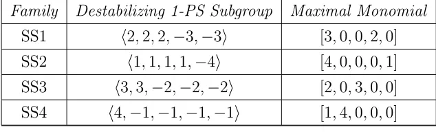
Using this procedure it is determined that the monomials [3,0,0,2,0], [4,0,0,0,1], [2,0,3,0,0], and [1,4,0,0,0] are the maximal monomials which have µ≤0.
Table 4.1: Strictly Semistable Families SS1 - SS4
Family Destabilizing 1-PS Subgroup Maximal Monomial
Figure 4.5: Poset structure of family SS4
Table 4.2: Strictly Semistable Families SS5 - SS7
Family Destabilizing 1-PS Subgroup Maximal Monomial
Figure 4.14: Poset structure of family SS7 III
monomials in each family can be used to give the general polynomial form for each family.
Remark 4.2.7. The polynomials will be written in the following forms
qa(xp. . . xr) polynomial of degree a in the variablesxp. . . xr qa,b(xp. . . xr kxt. . . xs) linear combination of monomials of degree a
inxp. . . xr and degree b inxt. . . xs
Proposition 4.2.8. Y is strictly semistable or unstable if it is equivalent, via coor-dinate transformation, to a hypersurfaces in one of the following families:
Table 4.3: Strictly Semistable Families SS1 - SS7
Family Destabilizing 1-PS Subgroup Maximal Monomial
SS1 h2,2,2,−3,−3i [3,0,0,2,0]
q3,2(x0, x1, x2kx3, x4) +q2.3(x0, x1, x2kx3, x4) +q1,4(x0, x1, x2kx3, x4) +q5(x3, x4)
SS2 h1,1,1,1,−4i [4,0,0,0,1]
x4q4(x0, x1, x2, x3, x4)
SS3 h3,3,−2,−2,−2i [2,0,3,0,0]
q2,3(x0, x1kx2, x3, x4) +q1,4(x0, x1kx2, x3, x4) +q5(x2, x3, x4)
SS4 h4,−1,−1,−1,−1i [1,4,0,0,0]
x0q4(x1, x2, x3, x4) +q5(x1, x2, x3, x4)
SS5 h1,0,0,0,−1i [0,5,0,0,0],[1,3,0,0,1],[2,1,0,0,2]
x2
0(x24q1(x1, x2, x3, x4)) +x0x4q3(x1, x2, x3, x4) +q5(x1, x2, x3, x4)
SS6 h4,4,−1,−1,−6i [1,0,4,0,0],[3,0,0,0,2],[2,0,2,0,1]
x2
4q3(x0, x1) +x4q2,2(x0, x1kx2, x3, x4) +q1,4(x0, x1kx2, x3, x4) +q5(x2, x3, x4) SS7 h6,1,1,−4,−4i [0,4,0,1,0][1,2,0,2,0][2,0,0,3,0]
x2
0q3(x3, x4) +x0(q2,2(x1, x2kx3, x4) +q1,3(x1, x2kx3, x4) +q4(x3, x4)) +q4,1(x1, x2k x3, x4) +q3,2(x1, x2kx3, x4) +q2,3(x1, x2kx3, x4) +q1,4(x1, x2kx3, x4) +q5(x3, x4) .
4.3
Unstable Families
families which makes it very tedious and not very illustrative. Another approach would be to find and characterize the minimal orbits as is done in Chapter 5. The idea of the minimal orbit approach is that each maximal semistable family will degenerate, via the destabilizing 1-PS λ, to a smaller family of hypersurfaces. It is then much easier to distinguish between unstable and strictly semistable hypersurfaces in the smaller family. See Chapter 5 for a complete characterization of strictly semistable and unstable orbits.
4.4
Bad Flags
Having found the maximal semistable families, one can give a geometric descrip-tion by characterizing the types of singularities found on a generic member of one of these families. The existence of a destabilizing 1-PS λ gives rise to a ”bad flag” of the vector spaces H0(P4,OP
4(1)) ∼=C5. A general principal given by Mumford ( [16]
p.48) is that these ”bad flags” pick out the singularities which cause the family to become semistable or unstable.
Using the approach given by Laza ( [12] p.7) it can be shown that a 1-PSλ:C∗
→
T gives a weight decomposition ofH0(P4,OP
4(1)) =⊕5
i=0Wi based on the eigenvalues of λ acting on H0(P4,OP4(1)).
Definition 4.4.1. For a 1-PS λ = ha, b, c, d, ei let mi be a subset of {a, b, c, d, e} which have the same weights and let ni be the weight.
Wmi :=
M
iwhereWihas eigenvalueni
Wi (4.10)
The standard flag is given by
∅ ⊆F1 = (x1 =x2 =x3 =x4 = 0)⊆F2 = (x2 =x3 =x4 = 0)⊆
F3 = (x3 =x4 = 0)⊆F4 = (x4 = 0)⊆P4
Definition 4.4.2. Given a 1-PS λ = ha, b, c, d, ei let m1, m2. . ., ms represent the collection of common weights of λ. Let mi be ordered by increasing value of weights (i.e. m1 has lowest weight). The associated flag for λ is
Fλ : ∅ ⊆Fms :=
s M
i=1
Wmi ⊂Fms−1 :=
s−1
M
i=1
Wmi ⊂. . .⊆Fm1 :=Wm1 ⊆P
4. (4.12)
This is a subflag of the standard flag (4.12).
For the maximal destabilizing families SS1-SS7 the associated ”bad flags” are Table 4.4: Destabilizing Flags of SS1-SS7
Family Destabilizing 1-PS Subgroup Flag Fλ
SS1 h2,2,2,−3,−3i ∅ ⊆(x3=x4= 0)⊆P4
SS2 h1,1,1,1,−4i ∅ ⊆(x4= 0)⊆P4
SS3 h3,3,−2,−2,−2i ∅ ⊆(x2=x3=x4= 0)⊆P4
SS4 h4,−1,−1,−1,−1i ∅ ⊆(x1=x2=x3=x4= 0)⊆P4
SS5 h1,0,0,0,−1i ∅ ⊆(x1=x2=x3=x4= 0)⊆(x4= 0)⊆P4 SS6 h4,4,−1,−1,−6i ∅ ⊆(x2=x3=x4= 0)⊆(x4= 0)⊆P4 SS7 h6,1,1,−4,−4i ∅ ⊆(x1=x2=x3=x4= 0)⊆(x3=x4= 0)⊆P4.
4.5
Geometric Interpretation of Maximal Semistable
Families
In order to determine the singularities of the families SS1-SS7 we can intersect the general form of the equation with the flag arising from its destabilizing 1-PS. This will give some description of the types of singularities which occur in each family. A precise description of each such family is given in the propositions below.
Proof. LetY be of type S1 then it is equivalent, via a coordinate transformation, to the hypersurface
q3,2(x0, x1, x2 kx3, x4) +q2.3(x0, x1, x2 kx3, x4)
+q1,4(x0, x1, x2 kx3, x4) +q5(x3, x4).
(4.13)
This hypersurface contains the ideal hx3, x4i2 which is a double plane inP4.
Let Y be a hypersurface which contains a double plane. By a coordinate trans-formation we can assume the double plane is hx3, x4i2. The most general equation
which contains the ideal hx3, x4i2 is (4.13).
Proposition 4.5.2. A hypersurface Y is of type SS2 if and only if Y is a reducible variety, where a hyperplane is one of the components. In particular, the singularity
is the intersection of the hyperplane with the other component which is generically a degree 4 surface.
Proof. LetY be of type S2 then it is equivalent, via a coordinate transformation, to the hypersurface
x4q4(x0, x1, x2, x3, x4) (4.14)
This hypersurface has the hyperplane hx4i as a component.
Let Y be a reducible hypersurface where a hyperplane is a component. The polynomialf ∈C[x0, x1, x2, x3, x4] definingY can be factored intof =gh, wherehis
a degree 1 polynomial. By a coordinate transformation we can map the hyperplane defining htox4. Without loss of generalityf =x4h. Since sincef is of degree 5 then
by neccesity h is of degree 4 thereforef is of the form (4.14).
Proof. Let Y be of type SS3 then it is equivalent, via a coordinate transformation, to the hypersurface
q2,3(x0, x1 kx2, x3, x4) +q1,4(x0, x1 kx2, x3, x4) +q5(x2, x3, x4) (4.15)
This hypersurface contains the ideal hx2, x3, x4i3 which is a triple line in P4.
LetY be a hypersurface which contains a triple line. By a coordinate transforma-tion, we can assume the triple line is hx2, x3, x4i3. The most general equation which
contains the ideal hx2, x3, x4i3 is (4.15).
Proposition 4.5.4. A hypersurface Y is of type SS4 if and only if Y contains a quadruple point.
Proof. Let Y be of type SS4 then it is equivalent, via a coordinate transformation, to the hypersurface
x0q4(x1, x2, x3, x4) +q5(x1, x2, x3, x4) (4.16)
This hypersurface contains the idealhx1, x2, x3, x4i4 which is a quadruple point inP4.
Let Y be a hypersurface which contains a quadruple point. By a coordinate transformation we can assume the quadruple point is hx1, x2, x3, x4i4. The most
general equation which contains the idealhx1, x2, x3, x4i4 is (4.16).
Proposition 4.5.5. A hypersurface Y is of type SS5 if and only if Y has a triple point p with the following properties:
i) the tangent cone of p is the union of a double plane and another hyperplane;
Proof. Let Y be of type SS5 then it is equivalent, via a coordinate transformation, to the hypersurface
x20
x24q1(x1, x2, x3, x4)
+x0x4q3(x1, x2, x3, x4) +q5(x1, x2, x3, x4) (4.17)
This hypersurface contains the triple point hx1, x2, x3, x4i3. The tangent cone is the
hypersurface defined by
x2
4q1(x1, x2, x3, x4) (4.18)
which is the union of a double hyperplane hx4i2 and another general hyperplane
q1(x1, x2, x3, x4). The points whose lines passing through the triple point which have
intersection multiplictity 5 with the hypersurface, is the locus ofhx2
4q1(x1, x2, x3, x4)i
andhx4q3(x1, x2, x3, x4)i. Sincex4 is a component of both terms then a line emanating
from the hyperplane hx4i to the triple point will have multiplicity 5.
Let Y be a hypersurface which contains a triple point. By a coordinate transfor-mation we can assume the triple point is hx1, x2, x3, x4i3. The most general equation
which contains the ideal hx1, x2, x3, x4i3 is
x2 0
q3(x1, x2, x3, x4)
+x0
q4(x1, x2, x3, x4)
+q5(x1, x2, x3, x4). (4.19)
If the tangent cone is the union of a double plane and another hyperplane then
q3(x1, x2, x3, x4) = f2g (4.20)
where f and g are linear forms. By a coordinate transformation which keeps the triple point fixed we can map the hyperplane f to x4. So without loss of generality
If a general line from the hyperplane hx4i to the triple point has multiplicity 5
then
x4 =q4 = 0. (4.22)
This occurs only if q4 has x4 as a component so
q4 =x4q3 (4.23)
which is precisely of the form (4.17).
Proposition 4.5.6. A hypersurface Y is of type SS6 if and only if Y has a double line L where every point p∈L has the following properties:
i) the tangent cone of each point p∈L is a double plane Pp;
ii) each point p∈L has the same double plane tangent cone i.e. Pp =P for some
double plane P;
iii) the line connecting the point on the tangent cone Pp and a point p ∈ L has
intersection multiplicty 4 with the hypersurface.
Proof. Let Y be of type SS6 then it is equivalent, via a coordinate transformation, to the hypersurface
q3(x0, x1)x24
+
x4q2,2(x0, x1 kx2, x3, x4)
+q1,4(x0, x1 kx2, x3, x4) +q5(x2, x3, x4)
(4.24)
This hypersurface contains the double linehx2, x3, x4i2. For any point [λ :ν : 0 : 0 : 0]
of the double line the tangent cone is the same double plane given by hx4i2. The
hx4i2 and hx4q2,2(λ, ν k x2, x3, x4)i. Since x4 is a component of both terms then the
line emanating from the hyperplane hx4i to any point of the double line will have
multiplicity 4.
Let Y be a hypersurface which contains a double line. By a coordinate trans-formation we can assume the double line is hx2, x3, x4i2. The most general equation
which contains the ideal hx2, x3, x4i2 is
q3,2(x0, x1 kx2, x3, x4) +q2,3(x0, x1 kx2, x3, x4) +q1,4(x0, x1 kx2, x3, x4) +q5(x2, x3, x4)
(4.25) If the tangent cone at every point on the double line is the same double plane then
q3,2(x0, x1 kx2, x3, x4) =q3(x0, x1)f(x2, x3, x4)2 (4.26)
where f is a linear form. By a coordinate transformation, which keeps the double line fixed, the hyperplane f is mapped to x2
4. So without loss of generality,
q3,2(x0, x1 kx2, x3, x4) = q3(x0, x1)x24. (4.27)
If the line going from the hyperplane hx4i to any point of the double line has
multiplicity 4 then
x4 =q2,3(λ, ν kx2, x3, x4) = 0. (4.28)
This occurs only if q2,3(x0, x1 kx2, x3, x4) has x4 as a component so
q2,3 =x4q2,2(x0, x1 kx2, x3, x4) (4.29)
Proposition 4.5.7. A hypersurface Y is of type SS7 if and only if Y contains a triple point p and a plane P, where p∈P has the following properties:
i) the tangent cone of p contains a triple plane of P;
ii) the singular locus of Y, when restricted to P, is the intersection of two quartic
curves q1 and q2;
iii) the point p is a quadruple point of q1 and q2.
Proof. Let Y be of type SS7 then it is equivalent, via a coordinate transformation, to the hypersurface
x2
0q3(x3, x4) +x0
q2,2(x1, x2 kx3, x4) +q1,3(x1, x2 kx3, x4) +q4(x3, x4)
+
q4,1(x1, x2 k x3, x4) +q3,2(x1, x2 kx3, x4) +q2,3(x1, x2 kx3, x4)
+q1,4(x1, x2 kx3, x4) +q5(x3, x4)
(4.30)
This hypersurface contains the triple point pgiven by the ideal hx1, x2, x3, x4i3 and a
plane P given by hx3, x4i. The tangent cone is the hypersurface defined byq3(x3, x4)
which which contains the triple plane hx3, x4i3 of P. When the differential of Y is
restricted to the plane hx3, x4ithe only non-trivial contribution comes from the term
q4,1(x1, x2 kx3, x4) = q4(x1, x2)x3+ ˜q4(x1, x2)x4. (4.31)
The differential, when restricted to the plane, is zero when
q4(x1, x2) = ˜q4(x1, x2) = 0. (4.32)
Therefore, the plane contains two quartic curves q4(x1, x2) and ˜q4(x1, x2) which
contain p as the quadruple point.
and the plane is hx3, x4i. The most general equation which contains the ideal
hx1, x2, x3, x4i3 and hx3, x4i is
x2 0
q2,1(x1, x2 kx3, x4) +q1,2(x1, x2 kx3, x4) +q3(x3, x4)
+x0
q3,1(x1, x2 kx3, x4) +q2,2(x1, x2 kx3, x4) +q1,3(x1, x2 kx3, x4) +q4(x3, x4)
+
q4,1(x1, x2 kx3, x4) +q3,2(x1, x2 kx3, x4) +q2,3(x1, x2 kx3, x4)
+q1,4(x1, x2 kx3, x4) +q5(x3, x4)
(4.33) If the tangent cone contains the triple plane ofP then it contains the idealhx3, x4i3.
Then the coeffecients of the x2
0 term of (4.33) contains only theq3(x3, x4) term. The
differential of (4.33), when restricted to the plane hx3, x4i, contains the equations of
the form x0q3(x1, x2) +q4(x1, x2) andx0q˜3(x1, x2) + ˜q4(x1, x2). If the singular locus of
Y in the plane is the intersection of two quartic curves then
x0q3(x1, x2) +q4(x1, x2) =x0q˜3(x1, x2) + ˜q4(x1, x2) = 0. (4.34)
So x0q3(x1, x2) +q4(x1, x2) and x0q˜3(x1, x2) + ˜q4(x1, x2) are the quartic curves. If
pis a quadruple point of both quartic curves thenq3 and ˜q3 are 0, so Y is of the form
(4.30).
4.6
Stable Locus
singularities which arise on the boundary of the moduli space. This gives some description of the singularities which arise in the stable locus. Ideally, the stable locus would only be smooth hypersurfaces and the boundary would include hypersurfaces with singularities. As shown in [1, 12] even in the case of cubic threefolds and cubic fourfolds this is not the case. As the degree and dimension of hypersurfaces increases more singularities will be included in the stable locus. In [16] there is a general proposition which states that a smooth hypersurface will always be stable.
Proposition 4.6.1 ( [16] Prop. 4.2). A smooth hypersurfaceF in Pn with degree≥2
is a stable hypersurface.
A complete classification of all possible singularities in the stable locus has not been found. Using the results of the previous section a partial list of singularities can be determined.
Proposition 4.6.2. If X is a quintic threefold with at worst a double point then it is stable.
Proof. SupposeX is not stable, then it is strictly semistable or unstable. So it belongs to one of the families SS1 - SS7, but X does not satisfy the singularity criteria for any of these families. Hence, it is stable.
Proposition 4.6.3. If X is a quintic threefold with at worst a triple point whose tangent cone is an irreducible cubic surface and X does not contain a plane then it
is stable.
Proof. SupposeX is not stable, then it is strictly semistable or unstable. So it belongs to one of the families SS1 - SS7. The only families which have at worst a triple point are families SS5 and SS7. Since the tangent cone ofX is irreducible then it is not in SS5. Since X does not contain a plane it is not in SS7, therefore it belong to neither family. Hence, it is stable.
Proof. SupposeX is not stable, then it is strictly semistable or unstable. So it belongs to one of the families SS1 - SS7. SS6 is the only family which has at worst a double line as a singularity. Since the tangent cone of X at each point is irreducible then it is not in SS6. Hence, it is stable.