INVESTIGATION
Evolutionary Branching in a Finite Population:
Deterministic Branching
vs.
Stochastic Branching
Joe Yuichiro Wakano*,†,1and Yoh Iwasa‡ *Meiji Institute for Advanced Study of Mathematical Sciences, Meiji University, Kawasaki 214-8571, Japan,†Japan Science and Technology, Precursory Research for Embryonic Science and Technology, Tokyo 102-8666, Japan, and‡Department of Biology, Kyushu University, Fukuoka 812-8581, Japan
ABSTRACT Adaptive dynamics formalism demonstrates that, in a constant environment, a continuous trait mayfirst converge to a singular point followed by spontaneous transition from a unimodal trait distribution into a bimodal one, which is called“evolutionary branching.”Most previous analyses of evolutionary branching have been conducted in an infinitely large population. Here, we study the effect of stochasticity caused by thefiniteness of the population size on evolutionary branching. By analyzing the dynamics of trait variance, we obtain the condition for evolutionary branching as the one under which trait variance explodes. Genetic drift reduces the trait variance and causes stochasticfluctuation. In a very small population, evolutionary branching does not occur. In larger popula-tions, evolutionary branching may occur, but it occurs in two different manners: in deterministic branching, branching occurs quickly when the population reaches the singular point, while in stochastic branching, the population stays at singularity for a period before branching out. The conditions for these cases and the mean branching-out times are calculated in terms of population size, mutational effects, and selection intensity and are confirmed by direct computer simulations of the individual-based model.
I
N addition to models using quantitative genetics (Lande 1981; Barton and Turelli 1991; Iwasaet al.1991; Pomiankowski et al.1991), adaptive dynamics formalism has revealed di-verse behaviors of evolutionary dynamics associated with continuous traits in various organisms (Metz et al. 1992; Dieckmann and Law 1996; Geritz et al. 1997, 1998). This approach allows us to analyze the evolution of many eco-logical traits for which frequency-dependent selection is prevalent without specifying the derlying genetic systems controlling the trait. Even in a perfectly constant environ-ment, a population may show intriguing temporal behavior. For example, if the trait evolves by accumulation of mu-tations of small magnitude and if the fitness is frequency dependent, a continuous trait may show convergence to a singular point followed by spontaneous splitting of a unimodal trait distribution into a bimodal (or multimodal) one, referred to as“evolutionary branching”(Metzet al.1992, 1996; Geritz et al.1997). Evolutionary branching is predicted to occurat an evolutionarily singular point that is approaching stable (or convergence stable, CS) but not evolutionarily stable (ES), and it is actually observed in individual-based simulations in many models for the evolution of ecologi-cal traits.
In evolutionary branching, an evolving population spon-taneously changes its trait distribution from unimodal to bimodal (or multimodal). Although evolutionary branching has been regarded as a model of sympatric speciation by some authors (Dieckmann and Doebeli 1999; Doebeli and Dieckmann 2000), the relationship between evolutionary branching in adaptive dynamics formalism and speciation events has been the focus of much debate (for review, see Waxman and Gavrilets 2005).
Most previous analyses of adaptive dynamics have assumed an infinite population size and that the fitness landscape acts as the deterministic driving force of evolu-tion. However, in afinite population, stochasticfluctuations are unavoidable. For example, an individual with a lower
fitness may be able to produce more offspring just by chance. Thus, a finite population can evolve against the selection gradient. As a result, stochasticity allows a popula-tion to jump from a low local peak to a higher peak. Hence, stochastic fluctuation can be an important factor in the outcome of evolution. The importance of stochasticity, or
Copyright © 2013 by the Genetics Society of America doi: 10.1534/genetics.112.144980
Manuscript received August 17, 2012; accepted for publication October 22, 2012 Available freely online through the author-supported open access option.
1Corresponding author: Meiji Institute for Advanced Study of Mathematical Sciences,
genetic drift, has been studied in detail in the context of quantitative population genetics (e.g., Lande 1976; Tazzyman and Iwasa 2000). On the other hand, in population genet-ics, random drift is known to decrease the genetic diversity of a population (e.g., Ewens 2004), which tends to slow down the action of natural selection. Hence, the effect of genetic drift is important to understand evolutionary dy-namics, including evolutionary branching, infinite popula-tions. In fact, Claessenet al.(2007) analyzed evolutionary branching in a model including three species and reported that genetic drift tends to cause a delay in evolutionary branching. However, a more detailed study of the relation-ship between evolutionary branching and genetic drift is needed.
In this article, we study the effect of stochasticfluctuation caused by the finiteness of population size (random genetic drift) on evolutionary branching. As an illustrative example, we adopt a model of a public goods game studied by Doebeli et al. (2004), who investigated evolutionary branching by using a corresponding individual-based simulation. The game model deals with a situation that is both biologically and socially interesting: a self-organized differentiation of play-ers into a highly cooperative group and a noncooperative group. Concerning the genetics, we in effect assume that the population is haploid and that the focal trait is con-trolled by a locus with many alleles. By focusing on this simplest case, we can analyze the effect of random genetic drift on the evolutionary outcome most clearly. We first show the results of individual-based simulations, using dif-ferent population sizes. We show that genetic drift is espe-cially important when the population size is small and that evolutionary branching does not necessarily occur even when the standard theory of adaptive dynamics predicts that it should. We also derive deterministic and stochastic ver-sions of the dynamics of the trait variance. We reveal that there are two different manners in which evolutionary branch-ing occurs: in deterministic branchbranch-ing, branchbranch-ing may occur quickly after the population reaches the singular point, while in stochastic branching, the population stays at a singularity for a period before branching out suddenly. We derive the conditions and mean branching-out times for these cases and confirm our predictions by direct computer simulations of the individual-based model.
Evolutionary Branching in a Game in a Finite Population
Individual-based model
As a full stochastic model of a population under natural selection, mutation, and random genetic drift, we consider the following stochastic process. The population consists of N individuals reproducing asexually. Each individual has a genetically determined trait value z2 ½0;1. At each dis-crete time stept, an individualiobtains a fecundityFifrom
pairwise interactions with the otherN21 individuals. Each interaction is a two-player game where a payoff given to an
individualimatched with an individualjis given byfðzi;zjÞ.
Its fecundityFiis denoted by
Fi¼
X
j6¼i
fðzi;zjÞ: (1)
Our framework is valid for any payoff functionfðzi;zjÞ. As an
example, we adopt a model by Doebeli et al. (2004) in which traitzrepresents the amount of investment into pub-lic goods shared by both players. In this game, the payoff function is represented by
fðzi;zjÞ ¼1þBðziþzjÞ2CðziÞ; (2a)
where the benefit function is
Bðz1þz2Þ ¼b1ðz1þz2Þ þb2ðz1þz2Þ2; (2b)
and the cost function is
CðzÞ ¼c1zþc2z2: (2c)
To keep the population size constant, the fitness of an individual with traitzi is denoted as
wðziÞ ¼
Fi
ð1=NÞPjFj: (3)
When the population size is infinitely large, Doebeli et al. (2004) have shown that the singular strategy z*¼ ðc12b1Þ=ð4b222c2Þ is convergence stable when
QCS¼4b222c2,0 and evolutionarily stable when
QES¼2b222c2,0. The singular strategy is referred to as
an evolutionary branching point whenQCS,0 andQES.0.
They have observed evolutionary branching in an individual-based simulation of a large population (N= 10,000).
In afinite population, the model includes random genetic drift, and the details of the updating rule and the order of different stages in population dynamics become impor-tant. Here, we assume a Wright–Fisher process. At each time step, fecundity is calculated for all N individuals. Then all individuals die and are replaced by their off-spring, which are sampled multinomially, with the prob-ability of an individual being the parent of each offspring individual proportional to the fecundity of the focal individual.
After reproduction, there is a small chance of mutationm, and the mutant has a trait value slightly different from that of the parent. To be specific, it follows a normal distribution with a mean equal to the parent’s and a variances2. Mutants
are constrained to be between 0 and 1, which confines traitz within an interval [0, 1].
Evolutionary branching depends on the population size
point). Thus, evolutionary branching is expected when the population size is infinitely large.
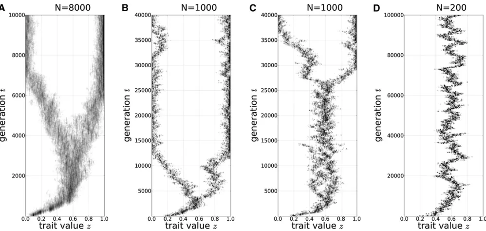
When the population size is large (N= 8000), evolution-ary branching occurs as soon as the trait evolves to reach the CS valuez* (Figure 1A). For an intermediate population size (N= 1000), the population lingers around the CS value,z*, before itfinally shows evolutionary branching. The waiting time until the evolutionary branching varies considerably among different simulation runs with the same parameter values (Figure 1, B and C). For a small population size (N = 200), we do not observe evolutionary branching and the population seems to stay around z*, even though z* is not evolutionarily stable (Figure 1D) (see also Wakano and Lehmann 2012).
The evolutionary branching dynamics are characterized by an abrupt increase or explosion of the variance of the focal phenotype (the trait variance). If all the parameters for the interactions are the same, a small population does not branch, an intermediately large population shows delayed branching, and a large population branches immediately. The intuitive reason for the smallness of the population size to suppress evolutionary branching is that genetic diversity is reduced by genetic drift every generation. In the following sections, we provide approximate dynamics for the trait variance to understand these simulation results.
Dynamics of Trait Variance
The full (individual-based) model is analytically intractable. Therefore, we derive a reduced simplified dynamical system here, which is tractable and gives predictions on the behavior
of the full model. One generation in the reduced model consists of two substeps.
Substep 1: Natural selection and mutation
LetuðzÞdenote a distribution of traitz, which is normalized to satisfyRuðzÞdz¼1. When afitness functionwðzÞis given and selection and mutation are sufficiently weak, the trait distribution in the offspring pool after mutation, denoted by
xðzÞ, can be approximated by the following replicator equa-tion plus a mutaequa-tion term,
xðzÞ ¼uðzÞ þwðzÞ2wuðzÞ þms
2
2
@2
@z2uðzÞ; (4)
where w is the population average of fitness values. The second term on the right-hand side represents the effect of selection and the third term represents the effect of muta-tion. The Taylor expansion of thefitness function around the average trait valuezis denoted as
wðzÞ¼wðzÞ þw1ðz2zÞ þw2 2ðz2zÞ
2; (5)
where the coefficients w1 and w2 are determined by the
current state z. The coefficientw1 represents the selection
gradient. The coefficientw2 indicates stabilizing selection if
it is negative and indicates disruptive selection if it is posi-tive. The derivation ofw2from the payoff functionfðzi;zjÞis
explained in Appendix A. For parameter values used in our simulations, we havew20:1, implying that disruptive
se-lection is operating. The population average and the vari-ance of trait values in the offspring trait distributionxðzÞare respectively denoted as
Avx½z¼zþw1m2þ
w2
2 m3; (6a)
Varx½z¼m22ðw12þw2
2Þm2
2þw
1m3þw2
2 m4þms
2;
(6b)
wheremkdenotes thekth centralized moment ofuðzÞ. The
above approximation is derived by neglectingm5 and
higher-order moments (seeAppendix B).
Substep 2: Random sampling (or random genetic drift)
From the offspring pool xðzÞ, N individuals are indepen-dently sampled to become adults. Hence, even for a fixed
xðzÞ, different distributions of adult phenotypes are realized according to a probability distribution (probability measure) over all possible trait distributions. After samplingN individ-uals independently fromxðzÞ, the expectation of the average trait value is identical to the average trait value inxðzÞ. In contrast, the expectation of the trait variance is decreased by a factor (N21)/N(Ewens 2004). Hence, we have the following:
E½Av½Z¼Avx½z
E½Var½Z¼N21 N Varx½z:
(7)
Combining the two substeps, the expected changes in the population average and the variance in one generation are given by
E½DAv½Z ¼w1m2þw2
2 m3; (8a)
E½DVar½Z ¼NN21hm2þw1m32w12m22þw2
2ðm42m2
2Þ þms2i2m 2:
(8b)
We are particularly interested in the dynamics of the variance of the trait distribution. To analyze Equation 8 further, we here assume that the trait distribution is close to a normal distribution whose mean and variance obey the dynamics given by Equation 8. For normal distributions,m3 ¼0 and
m4¼3m22. Using these relationships, we have the
follow-ing recursive equations for the mean and variance of the trait.:
Dz¼w1m2 (9a)
Dm2¼
N21
N ðw22w1
2Þm 222
1 Nm2þ
N21 N ms
2: (9b)
Thefirst, second, and third terms on the right-hand side of Equation 9b represent the effect of natural selection, the loss of diversity due to genetic drift, and the increase of diversity due to mutation, respectively. Without selection, the vari-ancem2 converges toðN21Þms2.
Condition for the Explosion of Trait Variance
As long as the selection gradient does not vanish (w1 6¼0),
the mean trait value changes according to Equation 9a, which is a standard result of population genetics (Ewens 2004) and corresponds to the canonical equation in adaptive dynamics theory (Dieckmann and Law 1996; Champagnatet al.2006). If a singular pointz*, where the selection gradient vanishes (w1 ¼0), is convergence stable, then the system approaches
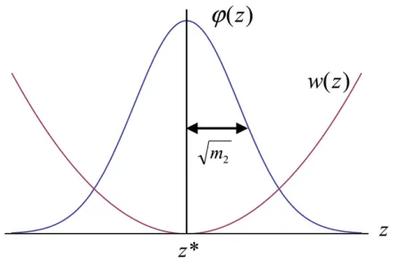
the singular point with time (Geritz et al.1997). Once the mean trait (i.e., thefirst moment of trait distribution) rea-ches the singularity, it will not change any longer. However, the trait variance (i.e., the second centralized moment of the distribution) may change with time. See Figure 2 for a sche-matic illustration. Here we focus on the recursion for the trait variance,
Dm2¼
N21 N w2m2
221
Nm2þ N21
N ms
2; (10)
which indicates that the one-generational change in the trait variance is equal to the sum of three terms: the natural se-lection term, the genetic drift term, and the mutation term. The right-hand side of Equation 10 represents the “force” acting on the trait variance (Figure 3). Note that the orders of the three terms in Equation 10 are m22, m2, and 1,
re-spectively. When the variance is small, the mutation (the third term) is dominant, and it increases the trait variance. As the variance increases, the genetic drift (the second term) in-creases its magnitude and it reduces the trait variance. The balance between these two processes would result in the equilibriumm2*Nms2, which represents the variance
de-termined by mutation–drift balance. When the trait variance is large, selection (thefirst term) becomes dominant. Selec-tion decreases the trait variance when w2,0 (stabilizing
selection), but it increases the trait variance when w2.0
(disruptive selection).
Combining these, we have three different cases, depend-ing on the parameters.
Case i: Whenw2,0, stabilizing selection is at work. Then the
dynamics of the trait variance (Equation10) have a single positive equilibrium
m2*5
1þ
ffiffiffiffiffiffiffiffiffiffiffiffiffiffiffiffiffiffiffiffiffiffiffiffiffiffiffiffiffiffiffiffiffiffiffiffiffiffiffiffiffiffiffi 124ðN21Þ2w2 ms2 q
2ðN21Þw2 ;
which is globally stable, and the trait variance converges to this value for any initial value. At this equilibrium, the trait variance is maintained by mutation, which increases variance, and by genetic drift and stabilizing selection, which decrease variance. Especially when the stabilizing selection is weak, trait variance converges to the level maintained by mutation– drift balance (m2* ðN21Þms2) whenjw2jis small.
Case ii: When 0,w2,1=4ms2ðN21Þ2, disruptive selection
one is stable, but the larger one is unstable. If the trait variance starts from a small value, it converges to the smaller equilibrium, where the trait variance is maintained mainly by the mutation–drift balance. If the trait vari-ance starts from a larger value, then disruptive selection dominates, leading to the unlimited growth of the trait variance.
Case iii: When w2.1=4ms2ðN21Þ2, disruptive selection is
strong. The dynamics of the trait variance no longer have a stable equilibrium. Starting from any initial value, the trait variance keeps increasing without limit.
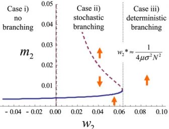
Figure 4 shows a bifurcation diagram of the variance dy-namics given by Equation 10, with the stabilizing/disruptive selection coefficient (w2) as a bifurcation parameter. Figure
5 shows a bifurcation diagram in which the population size (N) is a bifurcation parameter. We have a similar bifurcation diagram where mutational effects (ms2) serve as a bifurcation
parameter (not shown). We regard the explosion of the trait variance in the dynamics of Equation 10 as evolutionary branching. Then, these bifurcation diagrams show that evo-lutionary branching occurs as a result of a saddle-node bi-furcation. Evolutionary branching is predicted to occur at a non-ES singular point when disruptive selection intensity, population size, mutation rate, and mutation step size are sufficiently large. Specifically, the deterministic dynamics of Equation 10 predict that evolutionary branching occurs when 4ms2ðN21Þ2
w2.1 holds.
Stochastic Calculation of the Explosion of Variance
The deterministic dynamics of the trait variance repre-sented by Equation 10 indicate only the expectation of one-generational change. There must be stochasticity caused by the genetic drift. Results of an individual-based model, such as those illustrated in Figure 1, clearly show stochasticity. To account for stochasticity, the deterministic difference of Equation 10 needs to be modified by an additional term. In this section, we derive the stochastic differential
equa-tion model considering the stochasticity of trait variance dynamics.
The deterministic dynamics of Equation 10 can be ap-proximated by the ordinary differential equation (ODE)
d
dtm2¼fðm2Þ; (11a) where
fðxÞ ¼ðN21Þw2x
22xþ ðN21Þms2
N : (11b)
If stochasticity has no correlation over generations, and if the paths can be approximated as continuous, then we can incorporate the Brownian motion term, and the differential Equation 11 becomes the stochastic differential equation (SDE)
dM2¼fðM2Þdtþ ffiffiffiffi 2 N r
M2dB; (12)
wheredBdenotes Brownian motion andM2 denotes a
ran-dom variable representing the trait variance. fðM2Þ is the systematic change per generation in variableM2and is given
by Equation 11b.
The second term on the right-hand side of Equation 12 represents stochasticity in trait variance caused by random genetic drift (seeAppendix Cfor derivation). The stochastic
fluctuation term depends on the trait variance itself (geo-metric Brownian motion), because the amplitude of fl uctu-ation in the trait variance in each geneructu-ation of offspring is large when the trait variance in each parental generation is large. The stochastic term also depends on population size, because fluctuation is averaged out in large populations. Hence, random genetic drift becomes less important in larger populations. The system is similar to but different from the Figure 3 “Force”plotted against the trait variance based on Equation 10. Dotted, solid, and thick solid curves represent stabilizing selection (w2¼20.2), weak disruptive selection (w2= 0.2), and strong disruptive
selection (w2¼0.6), respectively. They also correspond to cases i, ii, and
iii in the main text. Parameters:N= 400,m50:01; s50:02. Figure 2 A schematic illustration of phenotype distributionuðzÞ and
fitness functionwðzÞwhen the mean trait valuezhas reached the
sin-gular strategyz*. The trait variance is Var½uðzÞ5m2so the standard
motion of a particle moved by force shown in Figure 3 under heat noise.
Stationary distribution
The corresponding Fokker–Planck equation (or forward Kol-mogorov equation) to Equation 12 is given by
@
@tpðm2;tÞ ¼ 2
@ @m2½
fðm2Þpðm2;tÞþ
1 2
@2 @m22
2 Nm2
2pðm 2;tÞ
(13)
(Feller 1971), where pðm2;tÞdm2¼Pr½m2#M2ðtÞ,m2þ
dm2 is the probability density for the trait variance m2.
The stationary distribution of the trait variance is
~
pðxÞ ¼C x23eðN21ÞaðxÞ; (14a)
whereCis a normalizing constant and
aðxÞ ¼w2x
22ms2
x : (14b)
Figure 6 illustrates an example of stationary distribution of the trait variance, showing that the system tends to show slightly smaller trait variance than the locally stable value in Equation 11, because the fluctuation is weaker when the variance is smaller (geometric Brownian motion).
Comparison with the results of simulations:We compared the stationary distribution of the trait variance between the theoretical prediction given by Equation 14 and the observed distribution obtained from the individual-based simulation (Evolutionary Branching in a Game in a Finite Population section). Figure 7 shows good agreement be-tween the diffusion approximation (i.e., the SDE model) and the corresponding simulation result with a small pop-ulation size. In particular, the approximation captures the shift of the mode—the peak of the distribution lies at the value smaller thanNms2¼0:0008. The average trait
var-iance in an interval shown in Figure 7 is close toNms2for
both analytic prediction (Equation 14) and simulation results.
Waiting time for evolutionary branching
In case ii, there are stable and unstable equilibria for the trait variance, the latter being larger than the former. If the initial value of trait variance is smaller than the unstable equilibrium, the deterministic model Equation 11 predicts that variance would be maintained indefinitely. In contrast, if the initial value is larger than the unstable equilibrium, it quickly increases and grows without limit. Hence, whether trait variance eventually explodes depends on the initial condition. In the presence of stochasticity, however, the trait variance would not be maintained at smaller values than the unstable equilibrium; instead, it wouldfluctuate around the stable equilibrium for a period, but then eventually increase beyond the unstable equilibrium and diverge to infinity. Hence, under the stochastic differential equation, the trait variance is predicted to explode eventually even if the initial value is small. The timing of this explosion is controlled by the stochasticity.
The mean waiting time prior to explosion is a typical “first passage time” problem in diffusion theory. This has also been used in calculating the mean time of fixation in population genetics (Kimura and Ohta 1968) and the mean time to extinction in conservation biology (e.g., Lande 1993; Hakoyama and Iwasa 2000) and physiology (e.g., Ricciardi and Smith 1977).
To study the expectation of waiting time, we assume that a system has a reflecting boundary at m2 ¼l0 and an
absorbing boundary atm2¼r(note that the left boundary
can never be achieved because the deterministic force is in-creasing the variance while stochastic fluctuation vanishes atm2¼0;i.e., Equation 12 is singular atm2¼0). LetTðhÞ
be the expected waiting time until the system reaches the right absorbing boundary m2¼rwhen the initial value of
the trait variance ism2ð0Þ ¼h. To obtainTðhÞ, we use the backward Kolmogorov equation
21¼fðhÞd dhTðhÞ þ
h2
N d2
dh2TðhÞ; (15)
Figure 5 Stable (solid) and unstable (dashed) branches of the trait variance m2with population sizeNas a bifurcation parameter. A Log plot is shown.
Arrows indicate the direction of systematic change in m2. Parameters: m50:01; s50:02; ðb1;b2;c1;c2Þ5ð6:0;21:4; 4:56;21:6Þ.
Figure 4 Stable (solid) and unstable (dashed) branches of the trait vari-ancem2with disruptive selection intensityw2as a bifurcation parameter.
Arrows indicate the direction of systematic change inm2. Parameters:N=
with the boundary conditions TðrÞ ¼0 and T9ðlÞ ¼0 (see Appendix E). The solution is
TðhÞ ¼N Z r
h
Z y
l
x23yeðN21ÞðaðxÞ2aðyÞÞdxdy; (16)
whereaðxÞis given by Equation 14b. The expected waiting time is smaller when the population size is larger, disruptive selection is stronger, or mutational effects are larger (see Appendix D).
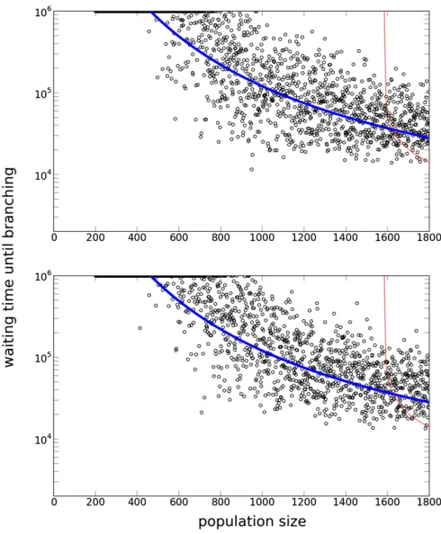
Comparison with the results of simulations:We compared the mean waiting times observed in the computer simulations of the individual-based model and the prediction by the ap-proximate stochastic differential equation model given by Equation 16. Once the system reaches a convergence stable point, the trait variance m2 is expected to be close to the
locally stable valueNms2(see also our results on stationary
distribution). Thus, we numerically calculateTðNms2Þ and
compare the corresponding result in individual-based simu-lation (Figure 8). We also derive the probability distribution of the first passage time by using Kolmogorov’s backward equation inAppendix E, but thefit of the shape of the prability distribution of waiting times to the distribution ob-served in individual-based simulations is less than perfect (Figure 9).
As we decrease N, the waiting time increases exponen-tially, and it eventually becomes impossible to escape from the locally stable unimodal state in a reasonable time (Figure 8). This implies that evolutionary branching is unlikely to occur in a small population.
When N is very large, genetic drift can be neglected and the system is approximated by the ODE: dm2=dt¼
w2m22þms2. Thus, the waiting time can be approximated
by the time required to move fromm2¼Nms2to the right
boundary m2¼r. This time is 1500 for N = 1000 and 960 for N= 2000. This calculation, in conjunction with
Figure 8, shows that the stochasticfluctuation plays a dom-inant role even in a population of 1000 individuals.
Our reduced model measures genetic diversity in trait distribution. An alternative measure of genetic diversity is the number of segregating alleles, which depends only onm and is predicted by Ewens’sampling formula when selection is absent (Ewens 2004). Figure 10 shows the effect of mu-tation rate m and mutation step size s2. Simulations con-firmed our prediction that only the value ofms2 matters,
even though the numbers of segregating alleles in the sim-ulation withN= 1800 were50 and150 form¼0.0025 and 0.01, respectively. It is also confirmed that smaller mu-tational effects require a longer waiting time until evolution-ary branching.
Discussion
In this article, we have studied the effect of stochastic
fluctuation due to finite population size on evolutionary branching. We have derived an ordinary differential equa-tion and then a stochastic differential equaequa-tion for the dy-namics of trait variance. The analysis has revealed that there are two different manners in which evolutionary branching occurs: deterministic branching and stochastic branching. In the case of deterministic branching, evolutionary branch-ing occurs relatively soon after the mean trait reaches the branching point. This occurs when disruptive selection in-tensityw2exceeds a threshold value,w2.1=ð4ms2ðN21Þ2Þ,
which can be approximated by 1=N,2 ffiffiffiffiffiffiffiffiffiffiffiffiffiffiw2ms2 p
. This con-dition for deterministic branching implies that the intensity of random genetic drift 1=N is smaller than disruptive selec-tion intensityw2and the mutational effectsms2 (see later in
article). If the opposite inequality holds,i.e., when disruptive selection is weaker than the threshold, then a unimodal dis-tribution is locally stable in the deterministic model and Figure 7 The stationary distribution of the trait variancem2. Curves
represent an analytic result (Equation 14), while bars are a histogram of realized trait variances in a simulation run for 106time steps. The dashed
line representsNms2= 0.0008. In the simulation, the initial trait
distribu-tion was set as monomorphic atz= 0.2. The transition from this initial state to the stationary state was negligible as it took only5000 time steps. Parameters: N = 200, m50:01; s50:02; ðb1;b2;c1;c2Þ5
ð6:0;21:4; 4:56;21:6Þ. Figure 6 The stationary distribution~pðm2Þof the trait variancem2
(Equa-tion 14). A Log-Log plot is shown, and thus the probability density is much higher at the peak than it appears. The locally stable value of the variance according to Equation 11 ism2*0.00081, which is close to
Nms2 = 0.0008 (dashed line). Note that a local peak lies at a value
,0.0008 because of geometric Brownian motion. Parameters:N= 200,
stochastic fluctuation is necessary for the population to undergo evolutionary branching. We call this latter type of evolutionary branching“stochastic branching.”We observed a relatively long waiting time until evolutionary branching occurs in simulations. The distribution and expectation of the waiting time were mathematically calculated and these predictions were consistent with computer simulations of the individual-based model. Considering the several assumptions we have adopted, the consistency is better than expected, although not perfect. As population size or mutational effect decreases, the waiting time exponentially increases. Mathe-matically, this is because these factors appear in the exponent in the expression of the expected waiting time (Equation 16). Although the increase of the waiting time is a continuous phenomenon resulting from the underlying stochasticity in individual-based simulations, we can understand evo-lutionary branching by classifying it as either determinis-tic branching in which stochasdeterminis-ticfluctuation is unnecessary or stochastic branching in which stochastic fluctuation is necessary.
Our analysis has revealed that evolutionary branching is almost impossible in some biological situations in which the effective population size or mutational effect is sufficiently small. As a population size increases, our condition for deter-ministic evolutionary branching approaches and converges to the standard branching-point condition. The condition can be written as 4w2N2ms2.1, which can be used as an
approxi-mate indicator; for example, a population with sizeN= 108
with mutational effects ms2 ¼10214 is predicted to show
deterministic branching when disruptive selection intensity is w2¼Oð1Þ, although such individual-based simulation is
almost impossible.
The condition separating deterministic and stochastic branching is understood intuitively by considering the force suppressing variance (genetic drift) and the two forces promoting the variance (disruptive selection and mutation). The balance between them determines which type of branching occurs. The condition for deterministic branching, 1=N,2 ffiffiffiffiffiffiffiffiffiffiffiffiffiffiw2ms2
p
can be rewritten as ð1=NÞ2,4w2ms2,
which means
ðgenetic driftÞ2,4·ðselection effectÞ·ðmutation effectÞ:
This implies that deterministic branching occurs when the intensity of genetic drift is smaller than double the geo-metric average of the selection and mutation intensities. It is important to note that the condition is determined by N2
instead ofN.
To mimic the full individual-based model by using the deterministic and stochastic equations of the trait variance, we have adopted several simplifying assumptions in deriving the dynamics:i.e., trait distribution is assumed to be close to normal, and the trait variance is small enough to justify series expansion. From simulation results, it is clear that the trait distributionfinally becomes multimodal when evo-lutionary branching occurs. Thus, our analytic results are valid only for the initial growth of the trait variance where unimodal distribution (approximated by a normal distribu-tion) becomes broader at the singular point. This initial explo-sion is followed by highly nonlinear and complex dynamics that realize a multimodal distribution. Nevertheless, the agree-ment of our analytic prediction and simulation results suggests that our reduced model captures the onset of evolutionary branching.
Based on individual-based simulations, Claessen et al. (2007) reported delayed evolutionary branching and pro-posed two reasons: random genetic drift and extinction of Figure 9 The distribution of waiting times. Curves represent an analytic result (seeAppendix E), while bars represent a histogram of the waiting time obtained in 1000 different runs of individual-based simulation. Parameters: N = 1000, m50:01; s50:02; ðb1;b2;c1;c2Þ5
ð6:0; 21:4; 4:56; 21:6Þ. Figure 8 A Log plot of waiting times for evolutionary branching for
different population sizes (N). The thick and thin curves represent analytic results based on a SDE model (Equation 16) and those based on an ODE model (Equation 11), respectively. Each open circle represents the result of a single run in individual-based simulation. The first time the trait variance exceeded 0.1 is shown. In the simulation, the initial trait distri-bution was set as monomorphic atz= 0.2 and each run consisted of 106
time steps. Simulation runs in which the variance did not explode are plotted at 106. Time required to reach a singular point in the simulation
was5000 whenN= 200 and2000 whenN= 1800, which is included to show open circles. Thus, open circles are expected to lie slightly above the curve. Parameters: m50:01; s50:02; ðb1;b2;c1;c2Þ5
incipient branches. In contrast to Claessenet al.(2007), our model has nofluctuation in the total population size. Thus, the delayed or absent evolutionary branching is caused by demographic stochasticity—thefluctuation in the number of offspring each individual produces. Our simple model has enabled us to derive the condition for evolutionary branch-ing mathematically, with random genetic drift taken into consideration, which has been only verbally proposed be-fore. In addition, our mathematical analysis and simulation results have revealed that the mutation rate and step size are as important as population size.
In this article, to illustrate the effect of genetic drift on the evolutionary branching, we used as an example a pair-wise interaction game that incorporated a Wright–Fisher update. We conjecture that the extension of our model to include a Moran update or to a multiplayer game is readily possible. In the case of including a Moran update, the loss of genetic diversity (Equation 7) should be appropriately mod-ified and also the unit of time should be rescaled since N Moran steps correspond to a single Wright–Fisher step. The result of our model should be easily extended to resource-competition models, which have been intensively studied in
adaptive dynamics (e.g., Dieckmann and Doebeli 1999; Sasaki and Dieckmann 2011; Mirrahimi et al.2012).
We have focused on the dynamic processes in which the population escapes from the locally stable value of the trait variance, while keeping its trait distribution as a unimodal distribution. Conceptually, if we allow all possible trait dis-tributions, we might have two locally stable states, one of which corresponds to a unimodal state and a second that corresponds to a fully branched state. Stochastic branching in the present model considers only the case in which a system located at the unimodal state escapes from this local optimum by stochastic fluctuation (random genetic drift). However, a branched state can also evolve back to the unimodal state by genetic drift; thus, a stochastic analysis including both escaping from and evolving back to the unimodal distribution would give us an even deeper un-derstanding of evolutionary branching.
Acknowledgments
We thank the following people for their very helpful com-ments: C. Hauert, Y. Kobayashi, C. Miura, W. Nakahashi, H. Ohtsuki, and A. Sasaki. This work was supported by Japan Science and Technology Precursory Research for Embryonic Science and Technology (J.Y.W.), by a Grant-in-Aid for Scientific Research (B) from Japan Society for Promotion of Science (to Y.I.), and also by the support of the Environment Research and Technology Development Fund (S9) of the Ministry of the Environment, Japan.
Literature Cited
Barton, N. H., and M. Turelli, 1991 Natural and sexual selection on many loci. Genetics 127: 229–255.
Champagnat, N., R. Ferriere, and S. Meleard, 2006 Unifying evo-lutionary dynamics: from individual stochastic processes to mac-roscopic models. Theor. Popul. Biol. 69: 297–321.
Claessen, D., J. Andersson, L. Persson, and A. M. de Roos, 2007 Delayed evolutionary branching in small populations. Evol. Ecol. Res. 9: 51–69.
Dieckmann, U., and R. Law, 1996 The dynamical theory of co-evolution: a derivation from stochastic ecological processes. J. Math. Biol. 34: 579–612.
Dieckmann, U., and M. Doebeli, 1999 On the origin of species by sympatric speciation. Nature 400: 354–357.
Doebeli, M., and U. Dieckmann, 2000 Evolutionary branching and sympatric speciation caused by different types of ecological in-teractions. Am. Nat. 156: S77–S101.
Doebeli, M., C. Hauert, and T. Killingback, 2004 The evolutionary origin of cooperators and defectors. Science 306: 859–862. Ewens, W. J., 2004 Mathematical Population Genetics.
Springer-Verlag, New York.
Feller, W., 1971 Introduction to Probability Theory and Its Appli-cation, Vol. 2, Ed. 3. John Wiley & Sons, New York.
Geritz, S. A. H., J. A. J. Metz, E. Kisdi, and G. Meszena, 1997 Dy-namics of adaptation and evolutionary branching. Phys. Rev. Lett. 78: 2024–2027.
Geritz, S. A. H., E. Kisdi, G. Meszena, and J. A. J. Metz, 1998 Evolutionarily singular strategies and the adaptive growth and branching of the evolutionary tree. Evol. Ecol. 12: 35–57.
Figure 10 A Log plot of waiting times for evolutionary branching for different population sizes and mutation parameters. The top panel (m50:0025;s50:02) depicts a result for a smaller mutation rate than in Figure 8, while the bottom panel (m50:01;s50:01) depicts a result for a smaller mutation step size. Asms251026is the same,
the analytic prediction curves are the same. The two simulation results are also undistinguishable. Parameters: ðb1;b2;c1;c2Þ5ð6:0;21:4;
Hakoyama, H., and Y. Iwasa, 2000 Extinction risk of a density-dependent population estimated from a time series of popula-tion size. J. Theor. Biol. 204: 337–359.
Iwasa, Y., A. Pomiankowski, and S. Nee, 1991 The evolution of costly mate preferences. 2. The handicap principle. Evolution 45: 1431–1442.
Karlin, S., and H. M. Taylor, 1981 A Second Course in Stochastic Processes. Academic Press, London.
Kimura, M., 1957 Some problems of stochastic processes in ge-netics. Ann. Math. Stat. 28: 882–901.
Kimura, M., and T. Ohta, 1969 The average number of genera-tions untilfixation of a mutant gene in afinite population. Ge-netics 61: 763–771.
Lande, R., 1976 Natural selection and random genetic drift in phenotypic evolution. Evolution 30: 314–334.
Lande, R., 1981 Models of speciation by sexual selection on poly-genic traits. Proc. Natl. Acad. Sci. USA 78: 3721–3725. Lande, R., 1993 Risks of population extinction from demographic
and environmental stochasticity and random catastrophes. Am. Nat. 142: 911–927.
Metz, J. A. J., R. M. Nisbet, and S. A. H. Geritz, 1992 How should we define “fitness” for general ecological scenarios? Trends Ecol. Evol. 7: 198–202.
Metz, J. A. J., S. A. H. Geritz, G. Meszena, F. J. A. Jacobs, and J. S. van Heerwaarden, 1996 Adaptive dynamics, a geometrical study of the consequences of nearly faithful reproduction,
pp. 183–231 inStochastic and Spatial Structures of Dynamical Systems, edited by S. J. van Strien and S. M. Verduyn Lunel. North-Holland Publishing, Amsterdam.
Mirrahimi, S., B. Perthame, and J. Y. Wakano, 2012 Evolution of species trait through resource competition. J. Math. Biol. 64: 1189–1223.
Pomiankowski, A., Y. Iwasa, and S. Nee, 1991 The evolution of costly mate preferences. 1. Fisher and biased mutation. Evolu-tion 45: 1422–1430.
Ricciardi, L. M., and C. E. Smith, 1977 Diffusion processes and related topics in biology, inLecture Notes in Biomathematics, Vol. 14. Springer-Verlag, Berlin.
Sasaki, A., and U. Dieckmann, 2011 Oligomorphic dynamics for analyzing the quantitative genetics of adaptive speciation. J. Math. Biol. 63: 601–635.
Tazzyman, S. J., and Y. Iwasa, 2000 Sexual selection can increase the effect of random genetic drift: a quantitative genetic model of polymorphism in Oophaga pumilio, the strawberry poison-dart frog. Evolution 64: 1719–1728.
Wakano, J. Y., and L. Lehmann, 2012 Evolutionary and conver-gence stability for continuous phenotypes infinite populations derived from two-allele models. J. Theor. Biol. 310: 206–215. Waxman, D., and S. Gavrilets, 2005 Twenty questions on
adap-tive dynamics. J. Evol. Biol. 18: 1139–1154.
Communicating editor: W. Stephan
Appendices
Appendix A: Fitness Function and the Coefficients
Because individuals are playing a game, their payoff and thus theirfitness depend not only on an individual’s own trait but also on their opponents’traits. In principle, it is impossible to determine afitness function for an individual with traitzby an average trait
zbecause more information is needed [i.e., the distribution of the traituðzÞ]. However, when the trait variance Var½uðzÞ ¼m2is
small,fitness is mainly determined by the deviation of the trait value from the average,z2zand can be approximated by
wðzÞ ¼wðzÞ þw1ðz2zÞ þw2 2ðz2zÞ
2;
(A1)
where the derivativesw1 andw2are evaluated at a situation for which all individuals (except self) carry the average traitz.
In other words, Equation A1 represents invasion fitness. The coefficients are functions of z, so that w1¼w1ðzÞ and
w2¼w2ðzÞ. According to adaptive dynamics, a singular point z* satisfies w1ðz*Þ ¼0 and it is convergence stable if ðd=dzÞw1ðzÞjz¼z*,0. It is evolutionarily stable ifw2ðz*Þ,0. When a singular point is convergence stable but not
evolution-arily stable, evolutionary branching is known to occur.
Here we mainly focus on a case in which the average trait remains atz¼z*, and thus we treatw1andw2as if they were
constant coefficients. They can be explicitly calculated forfiniteN, but whenN.100, it is well approximated by the value obtained by an infinite population limit. In this limit,fitness function is denoted as
wðzÞ ¼ fðz;z*Þ
fðz*;z*Þ; (A2)
and thus
w1¼ 1
fðz*;z*Þ
@
@zfðz;z*Þ
z¼z*
(A3a)
and
w2¼
1 fðz*;z*Þ
@2 @z2fðz;z*Þ
z¼z*
hold. To calculate the intensity of disruptive selection, not only the sign but also the magnitude is important. For the model of Doebeliet al.(2004), this becomes
w2¼
2ðb22c2Þ
fðz*;z*Þ ; (A4)
wherez*¼ ðc12b1Þ=ð4b222c2Þ. We numerically confirmed that the value ofw2can be well approximated byw20:1 for
the parameter values ðb1;b2;c1;c2Þ ¼ ð6:0;21:4; 4:56;21:6Þ and for the population sizes N .100. The magnitude of
disruptive selection depends on b1 andc1, as well as onb2 andc2. In the vicinity of our choice of parameter values used
in allfigures, disruptive selection is stronger for smaller values ofb1 and larger values ofc1.
Appendix B: Derivation of Deterministic Approximation
When both selection and mutation are weak, their effects can be approximated as additive and we obtain the replicator Equation 4. By integrating Equation 5, which is the Taylor expansion ofw(z) around
z[ Z
zuðzÞdz; (B1)
we have
w[ Z
uðzÞwðzÞdz¼wðzÞ þw2
2 m2; (B2)
where
mk[
Z
ðz2zÞkuðzÞdz (B3)
is thekth centralized moment aroundz. Putting this into Equation 4, we have
xðzÞ ¼uðzÞþ h
2w2
2 m2þw1ðz2zÞ þ w2
2ðz2zÞ
2iuð
z;tÞ þms
2
2
@2
@z2uðzÞ: (B4)
Imposing zero-flux boundary conditions@u=@z¼0, we have R
xðzÞdz¼1 R
xðzÞðz2zÞdz¼w1m2þw2
2 m3 R
xðzÞðz2zÞ2dz¼12w2 2 m2
m2þw1m3þw2
2 m4þms
2:
(B5)
We denote statistical values of the offspring distribution by
Avx½z[RxðzÞzdz
Varx½z[RxðzÞðz2Avx½zÞ2dz: (B6)
Then we have Avx½z ¼zþw1m2þ ðw2=2Þm3, which is Equation 6a.
To calculate the variance in the offspring pool, we use
Varx½z ¼RxðzÞz2zÞ2ðAvx½z2zÞ2dz
¼RxðzÞðz2zÞ2dz2ðw1m2þw2
2 m3Þ
2 (B7)
and we have
Varx½z ¼m22
w2
2 m2
2þw 1m3þ
w2
2 m4þms
22ðw 1m2þ
w2
2 m3Þ
2:
(B8)
When we neglect the fifth and higher-order terms, we have Varx½z ¼m22ðw12þw2=2Þm22þw1m3þ ðw2=2Þm4þms2,
Appendix C: Derivation of SDE Approximation
We want to approximate the dynamics by an SDE with the form
dM2¼fðM2Þdtþ
ffiffiffiffiffiffiffiffiffiffiffiffiffi gðM2Þ p
dB; (C1)
where dBdenotes Brownian motion and M2 denotes a random variable representing the variance in trait distribution. To
obtaingðxÞ, we use an established result in statistics that a random variable
X¼X
N
i¼1
Zi2z
v
2
(C2)
obeys the chi-square distribution whereZi’s areNindependent random variables each of which is sampled from a normal
distribution with mean z and variance v2. The variance of the chi-square distribution is 2N. When N is large, we can
approximatezin Equation C2 byZ. The trait variance M2can be written by
M2[
1 N
XN
i¼1
Zi2Z
2 ¼v2
N X; (C3)
whereM2 is a random variable, due to random genetic drift. Its variance over probability distribution is given by
Var½M2 ¼2N
v2
N
2 ¼2v4
N: (C4)
According to our model assumptions, we approximate the variance v2 by the trait variance in offspring distributionxðzÞ.
Then, we have the approximation
Var½M2 ¼2m2
2
N ; (C5)
which yieldsgðxÞ ¼2x2=Nand Equation 12.
By a more detailed calculation, we can show
Var½M2 ¼2ðN21Þm2
2
N2 ; (C6)
which results inp~ðxÞ ¼x2ð3N22Þ=ðN21ÞeNaðxÞ, but for our purpose Equation C5 is precise enough.
Appendix D: Properties of Waiting Times
Here, we show that the expectation of waiting time
T¼N Z r
h
Z y
l
x23yeðN21ÞðaðxÞ2aðyÞÞdxdy (D1)
is a decreasing function ofw2,N, andms2. First,Tis an increasing function ofaðxÞ2aðyÞ, which satisfies
aðxÞ2aðyÞ ¼ 2w2ðy2xÞ2ms2
1 x2
1
y : (D2)
Sincey.xholds in the region of integration in Equation D1, the waiting timeTis a decreasing function ofw2 andms2. To
show the dependence onN, we use
d dNT¼
Z r
h
Z y
l
where
Bðx;yÞ ¼yþNðx2yÞðwxyþms
2Þ
x : (D3b)
WhenNis large,B(x,y) has the same sign asx2y, which is negative. Thus,Tis a decreasing function ofNfor largeN. In addition, sinceaðxÞ2aðyÞis a negative constant independent ofN, we have
limN/NT¼0; (D4)
with all the other parametersfixed at positive values. This is true even for the vanishing mutation rate (i.e.,Nms2¼const:
whenN/N). However, it does not necessarily go to zero ifNðaðxÞ2aðyÞÞdoes not go to 2N. For example, ifNw2 and
Nms2 remain constant asN/N, the waiting timeTcan be an increasing function ofN.
Appendix E: Distribution of Waiting Times
LetcðxÞbe an indicator function such thatcðrÞ ¼1 andcðxÞ ¼0 forl#x,r. Then a random variablecðM2ðtÞÞis unity if absorption atm2¼rhas occurred until timet, and it is zero otherwise. Letuðh;tÞ ¼Eh½cðM2ðtÞÞ, where Eh denotes the
expectation in the stochastic process with the initial value M2ð0Þ ¼h. Then the following Kolmogorov backward equation
holds (Karlin and Taylor 1981):
@u
@t¼fðhÞ
@u
@hþ
1 2gðhÞ
@2u
@h2: (E1)
LetQbe a random variable representing thefirst passage time; then it is intuitively clear that
uðt;hÞ ¼Pr½Q#tjm2ð0Þ ¼h (E2)
is the probability that absorption atm2¼rhas occurred on or before timet. The probability density that absorption occurs
exactly at timetis given by@u=@t. A similar logic and calculation were adopted in a classical article studying thefixation probability in population genetics (Kimura 1957). The expectedfirst passage time is
TðhÞ ¼ Z N
0
t@u
@tdt: (E3)
After some calculations, we obtain
21¼fðhÞd dhTðhÞ þ
h2
N d2 dh2TðhÞ;