A Maximum-Likelihood Method to Correct for Allelic Dropout in Microsatellite Data with No Replicate Genotypes

INVESTIGATION

A Maximum-Likelihood Method to Correct

for Allelic Dropout in Microsatellite Data

with No Replicate Genotypes

Chaolong Wang,*,1_{Kari B. Schroeder,}†_{and Noah A. Rosenberg}‡ *Department of Computational Medicine and Bioinformatics, University of Michigan, Ann Arbor, Michigan 48109,†Centre for Behaviour and Evolution, Institute of Neuroscience, Newcastle University, Newcastle upon Tyne, NE2 4HH United Kingdom, and

‡_{Department of Biology, Stanford University, Stanford, California 94305}

ABSTRACTAllelic dropout is a commonly observed source of missing data in microsatellite genotypes, in which one or both allelic copies at a locus fail to be amplified by the polymerase chain reaction. Especially for samples with poor DNA quality, this problem causes a downward bias in estimates of observed heterozygosity and an upward bias in estimates of inbreeding, owing to mistaken classifications of heterozygotes as homozygotes when one of the two copies drops out. One general approach for avoiding allelic dropout involves repeated genotyping of homozygous loci to minimize the effects of experimental error. Existing computational alternatives often require replicate genotyping as well. These approaches, however, are costly and are suitable only when enough DNA is available for repeated genotyping. In this study, we propose a maximum-likelihood approach together with an expectation-maximization algorithm to jointly estimate allelic dropout rates and allele frequencies when only one set of nonreplicated genotypes is available. Our method considers estimates of allelic dropout caused by both sample-specific factors and locus-specific factors, and it allows for deviation from Hardy–Weinberg equilibrium owing to inbreeding. Using the estimated parameters, we correct the bias in the estimation of observed heterozygosity through the use of multiple imputations of alleles in cases where dropout might have occurred. With simulated data, we show that our method can (1) effectively reproduce patterns of missing data and heterozygosity observed in real data; (2) correctly estimate model parameters, including sample-specific dropout rates, locus-specific dropout rates, and the inbreeding coefficient; and (3) successfully correct the downward bias in estimating the observed heterozygosity. Wefind that our method is fairly robust to violations of model assumptions caused by population structure and by genotyping errors from sources other than allelic dropout. Because the data sets imputed under our model can be investigated in additional subsequent analyses, our method will be useful for preparing data for applications in diverse contexts in population genetics and molecular ecology.

M

ICROSATELLITE markers are widely used in popula-tion genetics and molecular ecology. In microsatellite data, distinct alleles at a locus represent DNA fragments of different sizes, typically detected by amplification using the polymerase chain reaction (PCR). Frequently, during micro-satellite genotyping in diploid organisms, one or both of an individual’s two copies of a locus fail to amplify with PCR, yielding a spurious homozygote or a spurious occurrence of missing data. This problem is known as“allelic dropout”(e.g.,

Gagneuxet al.1997; Pompanonet al.2005). For example, if an individual has genotype ABat a locus, but only alleleA successfully amplifies, then only alleleAwill be detected, and the genotype will be erroneously recorded as AA. If neither allelic copy amplifies, then the genotype will be recorded as missing. Here we follow Milleret al.(2002) by using“copies” to refer to the paternal and maternal variants in an individual and“alleles”to specify the distinct allelic types possible at a locus.

Allelic dropout is common in microsatellite studies and can lead to statistical errors in subsequent analyses (e.g., Bonin et al. 2004; Broquet and Petit 2004; Hoffman and Amos 2005). For example, in estimating population-genetic statistics, because allelic dropout can cause mistaken as-signment of heterozygous genotypes as homozygotes, it can lead to underestimation of the observed heterozygosity and Copyright © 2012 by the Genetics Society of America

doi: 10.1534/genetics.112.139519

Manuscript received March 7, 2012; accepted for publication July 17, 2012 Available freely online through the author-supported open access option. Supporting information is available online athttp://www.genetics.org/lookup/suppl/ doi:10.1534/genetics.112.139519/-/DC1.

1_{Corresponding author: University of Michigan, 100 Washtenaw Ave., 2017 Palmer}

overestimation of the inbreeding coefficient (Taberlet et al. 1999). Circumventing allelic dropout is therefore important for microsatellite studies. One general strategy for correct-ing for allelic dropout involves repeated genotypcorrect-ing, partic-ularly for the apparent homozygotes (e.g., Taberlet et al. 1996; Morinet al.2001; Wasseret al.2007). Additionally, computational approaches have been proposed to assess al-lelic dropout, primarily when replicate genotypes are avail-able (Miller et al.2002; Wang 2004; Hadfieldet al.2006; Johnson and Haydon 2007; Wrightet al.2009). In practice, however, replicate genotyping is costly and often uninforma-tive or impossible, owing to insufficient DNA or logistical constraints, especially for natural populations with limited DNA samples from noninvasive sources (e.g., Taberlet and Luikart 1999; Taberletet al.1999). Therefore, in this study, we develop a maximum-likelihood approach that can correct for allelic dropout without using replicate genotypes.

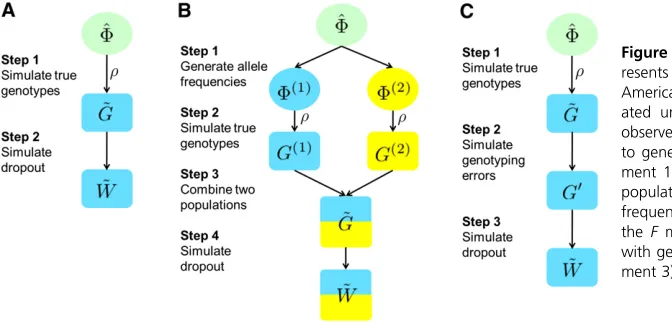
It is believed that the cause of allelic dropout is stochastic sampling of the molecular product, which can occur at two stages of the genotyping process (Figure 1). If DNA concen-tration is low, then one or both of the allelic copies might not be present in sufficient quantity for successful amplification (e.g., Navidi et al. 1992; Taberlet et al. 1996; Sefc et al. 2003). Poor quality of the template DNA (e.g., high degra-dation) can also prevent binding by the PCR primers and polymerase, resulting in dropout. An additional problem in the binding step is that some loci might be less likely than others to be bound. Previous studies have found that al-though different alleles at the same locus have similar prob-abilities of dropping out, loci with longer alleles tend to have higher dropout rates than those with shorter alleles (e.g., Sefc et al.2003; Buchanet al.2005; Broquet et al.2007); differences in primer annealing efficiency and in template DNA secondary structures might also contribute to different dropout rates across loci (Buchanet al.2005).

In this study, we explicitly model the two sources of allelic dropout, using sample-specific dropout rates gi and locus-specific dropout ratesgℓ, such that the probability of allelic dropout at locusℓof individualiis determined by a function of both giandgℓ. With a single nonreplicated set of geno-types, we jointly estimate the parameters of the model, in-cluding allele frequencies, sample-specific dropout rates, locus-specific dropout rates, and an inbreeding coefficient, thereby correcting for the underestimation of observed heterozygosity and overestimation of inbreeding caused by allelic dropout. We use an expectation-maximization (EM) algorithm to obtain maximum-likelihood estimates (MLEs). With the estimated parameter values, we perform multiple imputation to correct the bias caused by allelic dropout in estimating the observed heterozygosity. We have imple-mented this method in MicroDrop, which is freely available

athttp://rosenberglab.stanford.edu.

We first employ the method to analyze a set of human microsatellite genotypes from Native American populations. Using the estimated parameter values, we generate a simu-lated data set that mimics the Native American data, and we

employ this simulated data set to evaluate the performance of our model. First, we compare the patterns of missing data and heterozygosity between the simulated and real data to check whether our model correctly reproduces the observed patterns. Next, we compare estimated and true values of the allelic dropout rates for the simulated data. Finally, we compare the corrected heterozygosity with the“true”heterozygosity calculated from the true genotype data prior to allelic drop-out. We further evaluate the robustness of our model, using simulations with different levels of inbreeding, population structure, and genotyping errors from sources other than allelic dropout. We conclude our study by using simulations to argue that our MLEs of dropout rates and the inbreeding coefficient are consistent. That is, we show that as the num-ber of individuals and the numnum-ber of genotyped loci increase, our estimated values appear to converge to the true values of the parameters.

Data and Preliminary Analysis

The data set on which we focus consists of genotypes for 343 microsatellite markers in 152 Native North Americans collected from 14 populations over many years by the laboratory of D. G. Smith at the University of California (Davis, CA). We identify the populations according to their sampling locations: three populations from the Arctic/Sub-arctic region, two from the Midwest of the United States (US), two from the Southeast US, two from the Southwest US, three from the Great Basin/California region, and two from Central Mexico. In this data set, the number of distinct alleles per locus has mean 8.0 across loci, with a minimum of 4 and a maximum of 24.

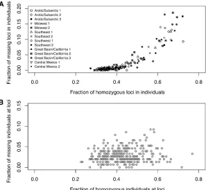
Allelic dropout can generate both spurious homozygotes, when one allelic copy drops out at a heterozygous locus, and missing data, when both copies drop out at either homozy-gous or heterozyhomozy-gous loci. Thus, under the hypothesis that missing data are caused by allelic dropout, we expect a higher proportion of missing data to be accompanied by a higher proportion of homozygous genotypes. If allelic drop-out is caused by low DNA concentration or low quality in certain samples, then a positive correlation will be observed across individuals between missing data and individual ho-mozygosity. Alternatively, if allelic dropout is caused by locus-specific factors such as differences across loci in the binding properties of the primers or polymerase, we instead expect a positive correlation across loci between missing data and locus homozygosity. This type of correlation is also expected if missing data are due to “true missingness”—for example, null alleles segregating in the population at certain loci, as a result of polymorphic deletions in primer regions (e.g., Pemberton et al. 1995; Dakin and Avise 2004). Here, we disregard true missingness and assume that all missing gen-otypes are attributable to allelic dropout.

For each individual, we evaluated the proportion of loci at which missing data occurred and the proportion of homo-zygotes among those loci for which data were not missing. As shown in Figure 2A, missing data and homozygosity have a strong positive correlation: the Pearson correlation isr= 0.729 (P,0.0001, by 10,000 permutations of the propor-tions of homozygous loci across individuals). This observa-tion matches the predicobserva-tion of the hypothesis that missing data result from sample-specific dropout rather than

locus-specific dropout or true missingness. By contrast, an analo-gous computation for each locus rather than for each individual (Figure 2B) finds that the correlation between homozygosity and missing data is much smaller (r = 0.099 and P = 0.0341, by 10,000 permutations of the proportions of ho-mozygous individuals across loci). We therefore suspect that missing genotypes in this data set arise primarily from the allelic dropout caused by low DNA concentration or quality in some samples and that locus-specific factors such as poor binding affinity of primers and polymerase have a smaller effect. In any case, for our subsequent analyses, we continue to consider both sample-specific and locus-specific factors.

Model

ConsiderNindividuals andLloci. Denote alleles at locusℓby Aℓkwithk= 1, 2,. . .,Kℓ, whereKℓis the number of distinct alleles at locusℓ. Denote the observed genotype data byW= {wiℓ:i= 1, 2,. . .,N;ℓ= 1, 2,. . .,L}, where genotyping has been attempted for all individuals at all loci. Here,wiℓis the observed genotype of theith individual at theℓth locus. Each entry ofWconsists of the two observed copies at a locus in a specific individual. If the observed genotype is missing at locusℓof individuali, then we specifywiℓ=XX. Otherwise, wiℓ=AℓkAℓhfor somek,h2{1, 2,. . .,Kℓ}, wherekandhare not necessarily distinct. The true genotypes are denoted by G= {giℓ:i= 1, 2,. . .,N;ℓ= 1, 2,. . .,L}. A description of the notation appears in Table 1.

To model the dropout mechanism, we specify a set of dropout statesZ= {ziℓ:i= 1, 2,. . .,N;ℓ= 1, 2,. . .,L} that

connects G and W and that indicates which alleles “drop out.” For a heterozygous true genotype giℓ = AℓkAℓh (h 6¼ k), supposing allele Aℓk drops out, the dropout state is ziℓ = AℓhX and the observed genotype is wiℓ = AℓhAℓh. For a homozygous true genotypegiℓ=AℓkAℓk, the dropout state ziℓ=AℓkX means that exactly one of the two allelic copies drops out.

We makefive assumptions in our model:

1. All distinct alleles are observed at least once in the data set.

2. All missing and incorrect genotypes are attributable to allelic dropout.

3. Both copies at a locus ℓ of an individual i have equal probabilitygiℓof dropping out. This probability is a func-tion of a sample-specific dropout rate gi. and a locus-specific dropout rategℓ:

g_iℓ¼g_iþg_ℓ2g_ig_ℓ: (1)

4. All individuals are unrelated and have the same inbreed-ing coefficientr, such that for any locus of any individual, the two allelic copies are identical by descent (IBD) with probabilityr.

5. Each pair of loci is independent (i.e., each pair of loci is at linkage equilibrium).

DenoteG= {gi,gℓ:i= 1, 2,. . .,N;ℓ= 1, 2,. . .,L} and F= {fℓk:ℓ= 1, 2,. . .,L;k= 1, 2,. . .,Kℓ}, in whichfℓk is the true frequency of alleleAℓkat locusℓ,giis the probability of dropout caused by sample-specific factors for any allelic copy at any locus of individuali, andgℓis the probability of dropout caused by locus-specific factors for any allelic copy at locusℓin any individual. Equation 1 arises by noting that the dropout probability for an allelic copy at locus ℓof in-dividuali, considering the two possible causes as indepen-dent, isgiℓ= 12(12gi)(12gℓ).

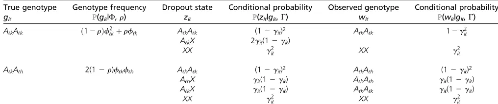
Using assumption 3, the conditional probabilityℙ(ziℓ| giℓ,G) can be expressed as shown in Table 2. The condi-tional probability of observing genotype wiℓ given true genotype giℓ and dropout ratesgi and gℓ can be calcu-lated as

ℙðwiℓjgiℓ;GÞ ¼

X

ziℓ

ℙðwiℓjziℓ;giℓÞℙðziℓjgiℓ;GÞ: (2)

Here, ℙ(wiℓ|ziℓ, giℓ) is either 0 or 1 becauseW is fully de-termined byZandG, and the summation proceeds over all dropout states ziℓpossible given the observed genotype wiℓ (Table 2).

We use a set of binary random variables S= {siℓ} to in-dicate the IBD states of the true genotypesG, such thatsiℓ= 1 if the two allelic copies in genotype giℓare IBD, andsiℓ=

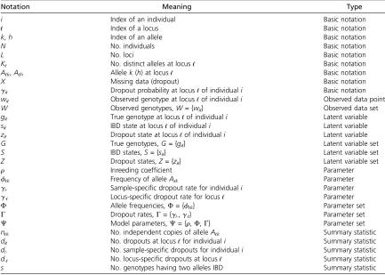
Table 1 Notation used in the article

Notation Meaning Type

i Index of an individual Basic notation

ℓ Index of a locus Basic notation

k,h Index of an allele Basic notation

N No. individuals Basic notation

L No. loci Basic notation

Kℓ No. distinct alleles at locusℓ Basic notation

Aℓk,Aℓh Allelek(h) at locusℓ Basic notation

X Missing data (dropout) Basic notation

giℓ Dropout probability at locusℓof individuali Basic notation

wiℓ Observed genotype at locusℓof individuali Observed data point

W Observed genotypes,W= {wiℓ} Observed data set

giℓ True genotype at locusℓof individuali Latent variable

siℓ IBD state at locusℓof individuali Latent variable

ziℓ Dropout state at locusℓof individuali Latent variable

G True genotypes,G= {giℓ} Latent variable set

S IBD states,S= {siℓ} Latent variable set

Z Dropout states,Z= {ziℓ} Latent variable set

r Inreeding coefficient Parameter

fℓk Frequency of alleleAℓk Parameter

gi Sample-specific dropout rate for individuali Parameter

gℓ Locus-specific dropout rate for locusℓ Parameter

F Allele frequencies,F= {fℓk} Parameter set

G Dropout rates,G= {gi,gℓ} Parameter set

C Model parameters,C= {r,F,G} Parameter set

nℓk No. independent copies of alleleAℓk Summary statistic

diℓ No. dropouts at locusℓfor individuali Summary statistic

di No. sample-specific dropouts for individuali Summary statistic dℓ No. locus-specific dropouts at locusℓ Summary statistic

s No. genotypes having two alleles IBD Summary statistic

0 otherwise. Under assumption 4, we have (e.g., Holsinger and Weir 2009)

ℙðsiℓjrÞ ¼

 r if siℓ¼1

12r if siℓ¼0 (3)

ℙðgiℓjsiℓ;FÞ ¼

8 > > > < > > > :

f2

ℓk if giℓ¼AℓkAℓkandsiℓ¼0     2f_ℓkf_ℓh if giℓ¼AℓkAℓhðh6¼kÞandsiℓ¼0

f_ℓk if giℓ¼AℓkAℓk and siℓ¼1 0 if giℓ¼AℓkAℓh ðh6¼kÞ andsiℓ¼1

(4)

ℙðgiℓjF;rÞ ¼

ð12rÞf2_ℓkþrf_ℓk if giℓ¼AℓkAℓk   2ð12rÞf_ℓkfℓh if giℓ¼AℓkAℓhðh6¼kÞ:

(5)

Whenr= 0, the genotype frequencies in Equation 5 follow Hardy–Weinberg equilibrium (HWE).

With the quantities in Equations 2–5, the probability of observingwiℓgiven parametersCis

ℙðwiℓjCÞ ¼

X

giℓ

ℙðwiℓjgiℓ;GÞℙðgiℓjF;rÞ: (6)

The summation proceeds over the set of all possible true genotypes giℓ, that is, over all two-allele combinations at locus ℓ. The likelihood function of the parameters C= {F,G,r} is then given by

ℙðWjCÞ ¼Y N

i¼1 YL

ℓ¼1

ℙðwiℓjCÞ: (7)

This likelihood assumes that dropout at a locus is inde-pendent across individuals, so that each observed diploid genotype of an individual at the locus is a separate trial independent of all others. Further, assumption 5 enables us to take a product across loci, as genotypes at separate loci are independent. A graphical representation of the rela-tionships among the parameters F, G, and r; the latent

variables G, S, and Z; and the observation W appears in Figure 3.

Estimation Procedure

Given the observed genotypes W, we can use an EM algo-rithm (e.g., Lange 2002) to obtain the MLEs of the allele frequencies F, the sample-specific and locus-specific drop-out ratesG, and the inbreeding coefficientr. Under the in-breeding assumption (assumption 4), two allelic copies at the same locus need not be independent. If two allelic copies are IBD, then the allelic state of one copy is determined given the allelic state of the other copy, so that the number of independent allelic copies is 1. If two copies at the same locus are not IBD, then the number of independent allelic copies is 2. We introduce a random variablenℓkto represent the number of “independent” copies of allele Aℓk in the whole data set, considering all individuals. We also define a random variablediℓas the number of copies that drop out at locusℓof individuali(diℓ= 0, 1, or 2).

In the E-step of our EM algorithm, we calculate (1) the expectation of the number of independent copies for all alleles, E[nℓk|W,C], summing across individuals; (2) for each indi-vidual, the total number of dropouts caused by sample-specific factors, E½dijW;C ¼PLℓ¼1E½diℓjW;Cðgi=giℓÞ; (3)

Table 2 Illustration of the outcomes of allelic dropout using two distinct alleles at locusℓ, AℓkandAℓh

True genotype Genotype frequency Dropout state Conditional probability Observed genotype Conditional probability

giℓ ℙ(giℓ|F,r) ziℓ ℙ(ziℓ|giℓ,G) wiℓ ℙ(wiℓ|giℓ,G)

AℓkAℓk ð12rÞf2ℓkþrfℓk AℓkAℓk (12giℓ)2 AℓkAℓk 12g2iℓ

AℓkX 2giℓ(12giℓ)

XX g2

iℓ XX g2iℓ

AℓkAℓh 2(12r)fℓkfℓh AℓhAℓk (12giℓ)2 AℓkAℓh (12giℓ)2

AℓhX giℓ(12giℓ) AℓhAℓh giℓ(12giℓ)

AℓkX giℓ(12giℓ) AℓkAℓk giℓ(12giℓ)

XX g2

iℓ XX g2iℓ

Genotype frequencies are calculated from allele frequencies using Equation 5, whereris the inbreeding coefficient, a parameter used to model the total deviation from Hardy–Weinberg equilibrium. Dropout is assumed to happen independently to each copy at locusℓof individuali, with probabilitygiℓspecified by Equation 1.h6¼k.

for each locus, the total number of dropouts caused by locus-specific factors, E½dℓjW;C ¼PNi¼1E½diℓjW;Cðgℓ=giℓÞ; and (4) the expectation of the total number of genotypes that are IBD, summing across the whole data set, E½sjW;C ¼ PN

i¼1

PL

ℓ¼1E½siℓjW;C. The factors gi/giℓ and gℓ/giℓ specify the respective probabilities that sample-specific factors and locus-specific factors contribute to the allelic dropouts at locus ℓof individuali.

To obtain the expectations required for the E-step, we need the posterior probabilities of giℓ, diℓ, and siℓ given the observed genotypewiℓand the parametersC, for each (i,ℓ) with i= 1, 2,. . .,Nandℓ= 1, 2,. . .,L. The posterior joint probabilities ofgiℓandsiℓgivenwiℓandCare listed in Table 3, and they are calculated from Bayes’formula:

ℙðgiℓ;siℓjwiℓ;CÞ

¼ ℙðgiℓ;siℓjCÞℙðwiℓjgiℓ;siℓ;CÞ P

giℓ P1

siℓ¼0ℙðgiℓ;siℓjCÞℙðwiℓjgiℓ;siℓ;CÞ

¼ _P ℙðsiℓjrÞℙðgiℓjsiℓ;FÞℙðwiℓjgiℓ;giℓÞ

giℓ P1

siℓ¼0ℙðsiℓjrÞℙðgiℓjsiℓ;FÞℙðwiℓjgiℓ;giℓÞ

:

(8)

The second equality holds because the probability of being IBD (siℓ= 1) depends only on the inbreeding coefficientr, the true genotype giℓ is independent ofr and the dropout rategiℓgivensiℓand the allele frequenciesF, and the observed genotypewiℓis independent ofFandrgivengiℓandgiℓ.

For example, suppose the observed genotype is wiℓ = AℓkAℓk, and we wish to evaluateℙ(giℓ=AℓkAℓk,siℓ= 1|wiℓ= AℓkAℓk,C), the posterior joint probability that the true geno-type isgiℓ=AℓkAℓkand the two allelic copies are IBD. Ifwiℓ= AℓkAℓkis observed, then the true genotypegiℓcan be a homo-zygoteAℓkAℓkor a heterozygoteAℓkAℓh, withh2{1, 2,. . .,Kℓ}

and h6¼ k. Each term in the summation in Equation 8 is a joint probabilityℙ(giℓ,siℓ,wiℓ|C). To calculate this quantity, ℙ(siℓ|r) andℙ(giℓ|siℓ,F) are obtained using Equations 3 and 4, respectively. The values ofℙ(wiℓ=AℓkAℓk|giℓ,giℓ) are given by Table 2 and can be obtained using Equation 2. The resulting probabilities ℙ(giℓ,siℓ,wiℓ|C) appear in Table 3. Therefore, for example,

ℙðgiℓ5AℓkAℓk;siℓ51jwiℓ5AℓkAℓk;CÞ

5ℙðgiℓ5AℓkAℓk;siℓ51;wiℓ5AℓkAℓkjCÞ

P

giℓ

P1

siℓ¼0ℙðgiℓ;siℓ;wiℓ¼AℓkAℓkjCÞ

5 rfℓk

12g2

iℓ _rf

ℓk1ð12rÞf2ℓk

12g2

iℓ1PKℓh¼1 h6¼k

2ð12rÞfℓkfℓhgiℓð12giℓÞ

5 rfℓk

12g2

iℓ _rf

ℓk1ð12rÞf2ℓk

12g2

iℓ

12ð12rÞf_ℓkð12f_ℓkÞg_iℓð12g_iℓÞ 5 rð11giℓÞ

rð11giℓÞ1ð12rÞð2giℓ2fℓkgiℓ1fℓkÞ:

(9) Table 3 Posterior joint probabilities of true genotypesgiℓand IBD statessiℓat a single locusℓof an individuali

Observed genotype

True

genotype IBD state Joint probability Posterior probability

wiℓ giℓ siℓ ℙ(giℓ,siℓ,wiℓ|C) ℙ(giℓ,siℓ|wiℓ,C)

AℓkAℓh AℓkAℓh 1 0 0

0 2(12r)fℓkfℓh(12giℓ)2 1

Others 1 0 0

0 0 0

AℓkAℓk AℓkAℓh 1 0 0

0 2(12r)fℓkfℓhgiℓ(12giℓ) 2ð12rÞfℓhgiℓ

rð1þgiℓÞ þ ð12rÞð2giℓ2fℓkgiℓþfℓkÞ

AℓkAℓk 1 rfℓkð12g2iℓÞ rð1þgiℓÞ

rð1þgiℓÞ þ ð12rÞð2giℓ2fℓkgiℓþfℓkÞ

0 ð12rÞf2

ℓkð12g2iℓÞ ð12rÞfℓkð1þgiℓÞ

rð1þgiℓÞ þ ð12rÞð2giℓ2fℓkgiℓþfℓkÞ

XX AℓkAℓh 1 0 0

0 2ð12rÞf_ℓkfℓhg2iℓ 2(12r)fℓkfℓh

AℓkAℓk 1 rfℓkg2iℓ rfℓk

0 ð12rÞf2

ℓkg2iℓ ð12rÞf2ℓk

The calculation ofℙ(giℓ,siℓ|wiℓ,C) is based on Equation 8.h6¼k.

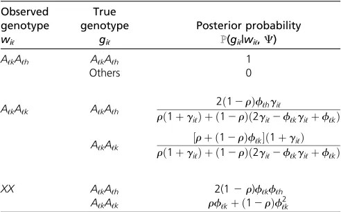
Table 4 Posterior probabilities of true genotypes giℓ at a single

locusℓof an individuali

Observed genotype

True

genotype Posterior probability

wiℓ giℓ ℙ(giℓ|wiℓ,C)

AℓkAℓh AℓkAℓh 1

Others 0

AℓkAℓk AℓkAℓh

2ð12rÞf_ℓhgiℓ

rð1þgiℓÞ þ ð12rÞð2giℓ2fℓkgiℓþfℓkÞ

AℓkAℓk ½

rþ ð12rÞf_ℓkð1þgiℓÞ rð1þgiℓÞ þ ð12rÞð2giℓ2fℓkgiℓþfℓkÞ

XX AℓkAℓh 2(12r)fℓkfℓh

AℓkAℓk rfℓkþ ð12rÞf2ℓk

With the values ofℙ(giℓ,siℓ|wiℓ=AℓkAℓk,C), the posterior probabilities ofgiℓandsiℓcan be easily calculated with Equa-tions 10 and 11, respectively. Results appear in Tables 4 and 5:

ℙðgiℓjwiℓ;CÞ ¼

X1

siℓ¼0

ℙðgiℓ;siℓjwiℓ;CÞ; (10)

ℙðsiℓjwiℓ;CÞ ¼ X

giℓ

ℙðgiℓ;siℓjwiℓ;CÞ: (11)

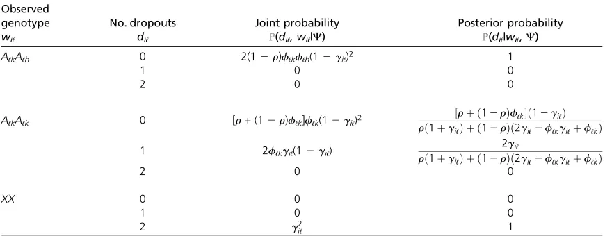
The posterior probabilities ofdiℓgivenwiℓandCappear in Table 6, and they are obtained by

ℙðdiℓjwiℓ;CÞ ¼ ℙð_ℙd_ðiℓ_w;wiℓjCÞ

iℓjCÞ ¼

ℙðdiℓ;wiℓjCÞ

P2

diℓ¼0ℙðdiℓ;wiℓjCÞ:

(12)

Here,

ℙðdiℓ;wiℓjCÞ ¼P

giℓ

ℙðdiℓ;wiℓ;giℓjCÞ

¼P

giℓ

ℙðdiℓ;wiℓjgiℓ;giℓÞℙðgiℓjF;rÞ

¼P

giℓ

ℙðwiℓjgiℓ;diℓÞℙðdiℓjgiℓÞℙðgiℓjF;rÞ: (13)

Therefore, E[nℓk|W, C], E[di|W, C], E[dℓ|W, C], and E[s|W,C] are calculated as

E½n_ℓkjW;C ¼ XN

i¼1 X

giℓ X1

siℓ¼0

fðA_ℓkjgiℓ;siℓÞℙðgiℓ; siℓjwiℓ;CÞ;

(14)

E½dijW;C ¼ XL

ℓ¼1 X2

diℓ¼0

diℓℙðdiℓjwiℓ;CÞ

g_i

g_iℓ; (15)

E½dℓjW;C ¼X N

i¼1 X2

diℓ¼0

diℓℙðdiℓjwiℓ;CÞg_gℓ

iℓ

; (16)

E½sjW;C ¼X N

i¼1 XL

ℓ¼1 X1

siℓ¼0

siℓℙðsiℓjwiℓ;CÞ; (17)

in whichf(Aℓk|giℓ,siℓ) indicates the number of independent copies of alleleAℓkin genotype giℓgiven the IBD statesiℓ, as defined below:

fðA_ℓkjgiℓ;siℓÞ ¼

8 > > > < > > > :

2 if giℓ ¼ AℓkAℓk andsiℓ¼0

1 if giℓ ¼ AℓkAℓk andsiℓ¼1 1 if giℓ ¼ AℓkAℓhðh6¼kÞ 0 otherwise:

(18)

Table 5 Posterior probabilities of the IBD statesiℓat a single locusℓ

of an individuali

Observed genotype

IBD

state Posterior probability

wiℓ siℓ ℙ(siℓ|wiℓ,C)

AℓkAℓh 1 0

0 1

AℓkAℓk 1

rð1þgiℓÞ

rð1þgiℓÞ þ ð12rÞð2giℓ2fℓkgiℓþfℓkÞ

0 ð12rÞð2giℓ2fℓkgiℓþfℓkÞ

rð1þgiℓÞ þ ð12rÞð2giℓ2fℓkgiℓþfℓkÞ

XX 1 r

0 12r

The calculation ofℙ(siℓ|wiℓ,C) is based on Equation 11.h6¼k.

Table 6 Posterior probabilities of the number of dropoutsdiℓat a single locusℓof an individuali

Observed

genotype No. dropouts Joint probability Posterior probability

wiℓ diℓ ℙ(diℓ,wiℓ|C) ℙ(diℓ|wiℓ,C)

AℓkAℓh 0 2(12r)fℓkfℓh(12giℓ)2 1

1 0 0

2 0 0

AℓkAℓk 0 [r+ (12r)fℓk]fℓk(12giℓ)2 _rð ½rþ ð12rÞfℓkð12giℓÞ

1þgiℓÞ þ ð12rÞð2giℓ2fℓkgiℓþfℓkÞ

1 2fℓkgiℓ(12giℓ) _rð 2giℓ

1þgiℓÞ þ ð12rÞð2giℓ2fℓkgiℓþfℓkÞ

2 0 0

XX 0 0 0

1 0 0

2 g2

iℓ 1

In the M-step of the EM algorithm, we update the estimation of parametersCby

f_ℓk¼ E½nℓkjW;C PKℓ

h¼1E½nℓhjW;C

for k¼1;2;. . .;Kℓ and

 ℓ ¼1;2;. . .;L; ₍₁₉₎

g_i¼E½dijW;C

2L for i¼1;2;. . .;N; (20)

g_ℓ¼E½dℓjW;C

2N for ℓ¼1;2;. . .;L; (21)

r¼E½sjW;C

NL : (22)

Justification of these expressions appears in Appendix A. With the updated parameter values, we calculate the likeli-hoodℙ(W|C) using Equation 7 and then repeat the E-step and the M-step. The likelihood is guaranteed to increase after each iteration in this EM process and will converge to a maximum (e.g., Lange 2002); the estimated parameter values are MLEs if this maximum is the global maximum. To lower the chance of convergence only to a local maximum, we repeat our EM algorithm with 100 sets of initial values of C. For each set, the allele frequencies, F = {fℓk: k = 1,

2,. . .,Kℓ;ℓ= 1, 2,. . .,L}, are sampled independently at

dif-ferent loci from Dirichlet distributions, Dirð1ð1Þ;1ð2Þ;. . .;1ðKℓÞÞ for locus ℓ; the sample-specific dropout rates gi (i = 1,

2,. . .,N), the locus-specific dropout ratesgℓ(ℓ= 1, 2,. . .,

L), and the inbreeding coefficientrare independently sam-pled from the uniform distributionU(0, 1). An EM replicate is considered to be “converged”if the increase of the

log-likelihood log10ℙ(W|C) in one iteration is,1024; when this

condition is met, we terminate the iteration process. The parameter values that generate the highest likelihood among the 100 EM replicates are chosen as our estimates.

Imputation Procedure

To correct the bias caused by allelic dropout in estimating the observed heterozygosity and other quantities, we create 100 imputed data sets by drawing genotypes from the posterior probability ℙðGjW;C^Þ ¼ℙðGjW;F^;G^;^rÞ, in which

^

F,G, and^ ^rare the MLEs ofF,G, andr, andℙ(G|W,C) is specified in Equation 10 and Table 4. In using this strategy, we not only impute the missing genotypes but also replace some of the observed homozygous genotypes with hetero-zygotes, as it is possible that observed homozygous geno-types represent false homozygotes resulting from allelic dropout. This imputation strategy accounts for the genotype uncertainty that allelic dropout introduces.

Application to Native American Data

We found that in sequential observations of the likelihood of the estimated parameter values, our EM algorithm con-verged quickly for all 100 sets of initial values forF,G, and r (results not shown). For each of the 100 sets, the EM algorithm reached the convergence criterion within 300 iter-ations. The difference in the estimated parameter values among the 100 replicates was minimal after convergence, indicating that the method was not sensitive to the initial values (results not shown).

Histograms of the estimated sample-specific dropout rates g^i and the estimated locus-specific dropout rates ^gℓ

appear in Figure 4. The mean of the g^i is 0.094, and for most individuals,g^i,0:1 (Figure 4A). The maximum^giis 0.405; this high rate indicates that some samples have low quantity or quality and is compatible with the fact that some of the samples are relatively old. Samples from some pop-ulations, such as Arctic/Subarctic 1 and Central Mexico 2, have higher overall quality, as reflected in low estimated sample-specific dropout rates.

Compared to the sample-specific dropout rates, the es-timated locus-specific dropout rates are much smaller, with mean 0.036 and maximum 0.160 (Figure 4B). The large spread of theg^i compared to the small values of theg^ℓ is consistent with the observation that the positive correlation between missing data and homozygotes is much greater across individuals than across loci (Figure 2).

The estimated inbreeding coefficient isr^¼0, the mini-mum possible value, smaller than the positive values typical of human populations. Several explanations could poten-tially explain the estimate of 0. First, our samples might be close to HWE. Second, our method might systematically un-derestimate the inbreeding coefficient, a hypothesis that we test below using simulations. Third, genotyping errors other than allelic dropout, such as genotype miscalling, can poten-tially also contribute to the underestimation. We use simula-tions to examine this hypothesis as well.

In a given individual, theLloci can be divided into three classes according to the observed genotypes:nhom

homozy-gous loci,nhetheterozygous loci, andL2nhom2nhetloci that

have both allelic copies missing. For each individual, we calculated the observed heterozygosity as Ho=nhet/(nhom+

nhet), as shown by gray symbols in Figure 4C. High

varia-tion exists inHofor different individuals, and the meanHo

across individuals is 0.590 (standard deviation = 0.137). The observed heterozygosities are negatively correlated with the MLEs of the sample-specific dropout rates (

Sup-porting Information, Figure S1), as is expected from the

underestimation of heterozygosity caused by allelic dropout. Averaging the estimated observed heterozygosity over 100 imputed data sets, we see that variation across individuals in estimated heterozygosities is reduced compared to the values estimated directly from the observed genotypes, and

the mean heterozygosity increases to 0.730 (standard de-viation = 0.035, Figure 4C). The estimated individual het-erozygosity does not vary greatly across different imputed data sets (standard deviation = 0.014, averaging across all individuals).

Simulations

We perform three sets of simulations to examine the per-formance of our method. First, we consider simulations that assume that the model assumptions hold, using as true values the estimated parameter values from the Native American data set (experiment 1). Next, we consider simulations that do not satisfy the model assumptions, by inclusion of popu-lation structure (experiment 2) and genotyping errors not resulting from allelic dropout (experiment 3). These latter simulations examine the robustness of the estimation pro-cedure to model violations.

Simulation methods

To generate simulated allelic dropout rates for use in experi-ments 2 and 3, we firstfit the distributions of the estimated sample-specific and locus-specific dropout rates from the Native American data, using beta distributions Beta(a,b). Denote the sample mean and sample variance of the MLEs of the sample-specific (or locus-specific) dropout rates asmandv, respectively. We estimated a and b using the method of moments, with ^

a¼m½mð12mÞ=v21 and b^¼ ð12mÞ½mð12mÞ=v21 (Casella and Berger 2001). The estimated sample-specific and locus-specific dropout rates approximately follow Beta (0.55, 5.30) and Beta(1.00, 27.00), respectively (Figure 4, A and B).

Experiment 1. Native American data: We simulate data under model assumptions 2–5 with parameter values esti-mated from the actual Native American data (results from Application to Native American Data). The simulation pro-cedure appears in Figure 5A. Suppose F,^ ^G, and ^r are the MLEs ofF,G, andrestimated from the data. First, we draw the true genotypesG, using probabilities speci~ fied by Equa-tion 5, assuming that the allele frequencies are given byF^

and the inbreeding coefficient by^r. Next, we simulate the dropout stateZ~by randomly dropping out copies with prob-ability specified by Equation 1, independently across alleles, loci, and individuals. Using G~ and Z, we then obtain our~ simulated observed genotypesW. This simulation approach~ does not guarantee that model assumption 1 will hold, be-cause some alleles might not be observed owing either to allelic dropout or to a stochastic failure to be drawn in the simulation. We simulate one set of genotypes atL= 343 loci forN= 152 individuals.

Experiment 2. Data with population structure:To test our method in a setting in which genotypes are taken from a structured population, we simulate data for two subpo-pulations with equal sample size (N1=N2= 76), genotyped

at the same set of loci (L= 343). We then apply our method on the combined data set, disregarding the population struc-ture. The procedure appears in Figure 5B.

First, we use theFmodel (Falushet al.2003) to generate allele frequencies for two populations that have undergone a specified level of divergence from a common ancestral population. We use the MLEs of the allele frequencies of the 343 loci in the Native American data (results from Ap-plication to Native American Data) as the allele frequencies of the ancestral population,FðAÞ¼F. Denote the estimated^ allele frequencies at locus ℓ by a vector f^_ℓ. Under the F model, allele frequencies of locus ℓ for population 1, fð_ℓ1Þ, and for population 2,fð_ℓ2Þ, are independently sampled from the Dirichlet distribution Dirððð12FÞ=FÞf^_ℓÞ, in whichFis a parameter constant across loci that describes the divergence of the descendant populations from the ancestral popula-tion.Fcan differ for populations 1 and 2, but for simplicity, we set F to the same value for both populations. Using Equations B1 and B2 in Appendix B and the independence offð_ℓk1Þandf

ð2Þ

ℓk , the squared difference of allele frequencies between the two populations satisfies E½ðfð_ℓk1Þ2f

ð2Þ ℓk Þ

2 ¼

2Ff^_ℓkð12f^ℓkÞ, which is linearly proportional to F. In the limit as F/0, we get fð_ℓ1Þ¼f_ℓð2Þ¼f^_ℓ for eachℓ, so that no divergence exists between either descendant population and the ancestral population.

We choose six values ofF(0, 0.04, 0.08, 0.12, 0.16, and 0.20) in different simulations. For each value, wefirst gen-erate allele frequencies, F(1) _{and F}(2)_{, at all 343 loci for}

populations 1 and 2. Next, we draw genotypes separately for each population according to the genotype frequencies in Equation 5, with the same value of the inbreeding coeffi -cientr. We consider 16 values forr, ranging from 0 to 0.15 in increments of 0.01. In total, we generate 6·16 = 96 sets of simulated genotypes with different combinations of set-tings for F andr (although for ease of presentation, some plots show only 36 of the 96 cases). Finally, we simulate allelic dropout on each of the simulated genotype data sets using giandgℓsampled independently from a Beta(a,b) distribution, in whicha= 0.55 andb= 5.30 are estimated from the MLEs of sample-specific dropout rates of the Native American data (Figure 4A). We do not use the estimateda

andbfrom the MLEs of locus-specific dropout rates because these MLEs lie in a relatively small range (Figure 4B) that would not permit simulation of high dropout rates for testing our method. Instead, use of the same beta distribution esti-mated from the sample-specific dropout rates produces a greater spread in the values of the simulated true locus-specific dropout rates, providing a more complete evaluation.

Experiment 3. Data with other genotyping errors: In our third experiment, we simulate data with stochastic genotyping errors other than allelic dropout. The simulation procedure appears in Figure 5C. Each simulated data set contains a single population of N= 152 individuals geno-typed for L = 343 loci. True genotypes are drawn with probabilities calculated from Equation 5, with allele fre-quencies F chosen as the maximum-likelihood estimated frequencies from the Native American data, and the inbreed-ing coefficientrranging from 0 to 0.15 incremented in units of 0.01 for different simulated data sets. Next, we simulate genotyping errors using a simple error model, in which at a K-allele locus in the simulated true genotypes, any allele can be mistakenly assigned as any one of the other K21 alleles, each with the same probability of e/(K 2 1). The parameterespecifies the overall error rate from sources other than allelic dropout, such as genotype miscalling and data entry errors (e.g., Wang 2004; Johnson and Haydon 2007). We consider six values fore(0, 0.02, 0.04, 0.06, 0.08, and 0.10), such that we simulate 96 (= 6 ·16) data sets with different combinations of e and r. In the last step, as in experiment 2, we simulate allelic dropout in each data set with both sample-specific and locus-specific dropout rates independently sampled from a Beta(0.55, 5.30) distribution.

Simulation results

We can formally compare the estimated dropout rates for the simulation with the true dropout ratesG~specified by the MLEs of the dropout rates for the Native American data. Figure 7A shows that our method accurately estimates the sample-specific dropout rates for all 152 individuals (mean squared error 2.6·1024_{). The estimated locus-specific}

drop-out rates are also close to their true values, but with a slightly higher mean squared error of 5.2·1024_{(Figure 7B). This}

difference between the estimation of sample-specific drop-out rates and that of locus-specific dropout rates can be explained by the fact that the number of loci (L= 343) is more than twice the number of individuals (N = 152).

Figure 6 Fraction of observed missing datavs.fraction of observed homozygotes for one simulated data set. (A) Each symbol represents an individual with fraction x of its nonmissing loci observed as homozygous and fraction yof its total loci observed to have both copies missing. The Pearson correlation betweenX andYisr= 0.900 (P, 0.0001, by 10,000 permutations ofXwhilefixingY). (B) Each point represents a locus at which fractionxof indi-viduals with nonmissing genotypes are observed to be homozygotes and fractionyof all individuals are observed to have both copies missing.r= 0.143 (P= 0.0045).

Consequently, more information is available for estimating a sample-specific rather than a locus-specific dropout rate. For the inbreeding coefficientr, our estimated value is 1.7· 1025_{, close to the true value of 0 that we used to generate}

the simulated genotypes.

Finally, in Figure 7C, we can see that our method suc-cessfully corrects the bias in estimating heterozygosity from the simulated data. The true observed heterozygosity is cal-culated using the true genotypes G~ and has mean 0.716, averaging across all individuals. The mean estimated ob-served heterozygosity, obtained from the obob-served uncor-rected genotypes W, is 0.565, lower than the true value.~ With imputed data sets, we obtain corrected heterozygosi-ties that are close to the true values. The mean and standard deviation of the corrected heterozygosities, evaluated from 100 imputed data sets and averaged across individuals, are 0.715 and 0.014, respectively. The low standard deviation across different imputed data sets indicates that our impu-tation strategy is relatively robust in correcting the underes-timation of observed heterozygosity.

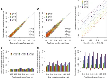
Experiment 2. Data with population structure:To further test the robustness of our method, we applied our method to 96 simulated data sets with different levels of population structure (parameterized byF) and inbreeding (parameter-ized byr). In Figure 8, A and C, we compare the estimated dropout rates to their true values. Considering the 36 sim-ulated data sets that are displayed, our method accurately estimates both the sample-specific and the locus-specific drop-out rates. The accuracy of our estimates is then quantified by mean squared errors for each simulated data set separately, as displayed in Figure 8, B and D. The performance in estimating the sample-specific dropout rate is not greatly affected by either the degree of population structure or the level of in-breeding (Figure 8B). By contrast, while the mean squared error of the estimated locus-specific dropout rates is roughly constant for different levels of inbreeding, it increases with the degree of population structure (Figure 8D).

One possible explanation for this observation is that the accuracy of allelic dropout estimates is closely related to the accuracy of the estimated allele frequencies. This accuracy

may decrease as the level of population structure increases, because we do not incorporate population structure in our model for estimation. The estimation of locus-specific dropout rates is more sensitive to inaccurate estimates of allele fre-quencies because the estimated accuracy of a locus-specific rate relies on the estimation of allele frequencies at that particular locus. By contrast, a sample-specific dropout rate is obtained by averaging the expected number of sample-specific dropouts across all loci in an individual and is less dependent on the accuracy of estimated allele frequencies at any particular locus. Therefore, sample-specific dropout rate estimates are less sensitive to population structure than are locus-specific estimates. When F = 0, with no population structure, the difference between the mean squared error for the sample-specific rates and that for the locus-specific rates arises simply from differences in the numbers of loci and individuals, as discussed for experiment 1.

Figure 8E shows the estimated inbreeding coefficient for all 96 simulated data sets, compared to the simulated true inbreeding coefficient in the subpopulations. With F = 0, a scenario for which no population structure exists and the data are generated under model assumptions 2–5, our method tends to slightly underestimate the inbreeding co-efficient. AsFincreases, the estimate becomes greater than the simulated inbreeding coefficient (Figure 8F). This result is consistent with our expectation, because according to the Wahlund effect (e.g., Hartl and Clark 1997), a pooled pop-ulation consisting of two subpoppop-ulations is expected to have more homozygous genotypes than an unstructured popula-tion, resulting in a pattern similar to that caused by a higher level of inbreeding within the unstructured population. In-deed, with no allelic dropout, a structured population under the F model has identical expected allele frequencies and genotype frequencies to those of an unstructured population with a higher inbreeding coefficientr* = r + (1 2r)[F/ (22F)] (Appendix B). By comparing our estimated inbreed-ing coefficient^r with the“effective inbreeding coefficient” r* (dashed lines in Figure 8E), we find that most of our estimated inbreeding coefficients are slightly smaller than the correspondingr*, indicating that the MLE ofris biased downward. It is worth noting that with a single parameterr, we capture the deviation of genotype frequencies from HWE introduced by population structure, thereby obtaining accu-rate estimated allelic dropout accu-rates without explicitly incor-porating population structure in our model.

We applied the imputation procedure to correct the bias in estimating heterozygosity for each of the 96 simulated data sets. Similarly to our application in experiment 1, we calculated the uncorrected and true heterozygosities for each individual from the simulated observed genotypes W~ and the simulated true genotypes G, respectively. The cor-~ rected heterozygosity was averaged across 100 imputed data sets for each simulated data set. Results for 36 simu-lated data sets appear inFigure S2, in which heterozygosi-ties were averaged across all individuals in each data set. Our results show a significant improvement of the corrected

heterozygosity over the uncorrected heterozygosity in all simulations, in that the corrected heterozygosity is consid-erably closer to the true heterozygosity. This improvement is fairly robust to the presence of population structure.

Experiment 3. Data with other genotyping errors:This set of simulations tested our method at different levels of genotyping error from sources other than allelic dropout. In all simulated data sets, with genotyping error ranging from 0 to 10% and rranging from 0 to 0.15, our method is successful in estimating both sample-specific and locus-specific dropout rates (Figure 9, A and C). The estimation accuracy of dropout rates is not strongly affected by the genotyping error rate (Figure 9, B and D). We can again see that a smaller number of individuals than loci has led to higher mean squared error for estimated locus-specific rates (Figure 9D) than for sample-specific rates (Figure 9B). Similar to theF= 0 case in our simulations with population structure, the simulated data sets with no genotyping error (e= 0) are generated under model assumptions 2–5. Consistent with the results forF= 0, our method slightly underestimates the inbreeding coefficientrfor most simulated data sets with e= 0. As genotyping error increases, the underestimation also increases (Figure 9, E and F). This result can be explained by noting that the simulated genotyping error, which changes the allele frequencies only slightly, tends to create false heterozy-gotes more frequently than false homozyheterozy-gotes. Therefore, the observed heterozygosity is increased while the expected hetero-zygosity changes little, leading to a decrease in the estimated inbreeding coefficient. Although our estimation of the inbreed-ing coefficient r becomes less accurate when the genotyping error rate is higher, the underestimation ofrdoes not prevent the method from accurately estimating allelic dropout rates.

For the heterozygosity, the corrected values obtained using our imputation strategy are closer to the true values than are the uncorrected values directly obtained from the observed genotypes (Figure S3). However, as the genotyping error rate eincreases, our method starts to overcorrect the downward bias in estimating the observed heterozygosity, and the cor-rected values exceed the true values. Similar to our explana-tion for the underestimaexplana-tion of the inbreeding coefficient, this overcorrection is introduced by the simulated genotyping er-ror, which creates an excess of false heterozygotes. This ex-cess is in turn incorporated into the corrected estimates of heterozygosity, because we do not model genotyping errors other than those due to allelic dropout.

Discussion

empirical missing data rates or excluding samples and loci with large amounts of missing data. Investigators can then use the imputed data in subsequent analyses, such as in studies of genetic diversity or population structure, or in software that disallows missing values in the input data. We have demonstrated our approach using extensive analyses of an empirical data set and data sets simulated using parameter values chosen on the basis of the empirical example.

We have found that our method works well on simulated data. In particular, it performs well in estimating the sample-specific dropout ratesgiand locus-specific dropout ratesgℓ. Further, in the examples we have considered, it is reasonably robust to violations of the model assumptions owing to the existence of population structure or to sources of genotyping error other than allelic dropout. This robustness arises partly from the inclusion of the inbreeding coefficient r in our model, which enables us to capture the deviation from HWE caused by multiple factors, such as true inbreeding, population structure, and genotyping errors. Because the various sources of deviation from HWE are incorporated into the single parameter r, the estimation of r itself is more sensitive to violation of model assumptions; therefore, it is important to be careful when interpreting the estimated value ofr, as it may reflect phenomena other than inbreed-ing. When data are simulated under our model, such as in the cases ofF= 0 ande= 0, our method tends to slightly

underestimate r (Figures 8E and 9E), indicating that our MLEs are biased, at least for the inbreeding coefficient.

We can use simulation approaches to further explore the statistical properties of our estimates. To examine the con-sistency of the estimators, we performed two additional sets of simulations, in which we generated genotype data under our model with either different numbers of individualsNor different numbers of loci L (Appendix C). When L is fixed, although estimates of the sample-specific dropout rates gi are not affected by the value of N, our estimates of the locus-specific dropout ratesgℓand the inbreeding coefficient rbecome closer to the true values asNincreases (Figure S4). WhenNis sufficiently large (e.g.,N= 1600), the estimates of g_ℓandrare almost identical to the true values. If we instead fixNand increaseL, then the estimates ofgiandreventually approach the true values, while the estimates of gℓ remain unaffected (Figure S5). These results suggest, without a strict analytical proof, that our MLEs of the dropout rates and in-breeding coefficient are likely to be consistent.

same 343 loci as were genotyped in our data. We obtained a meanHoof 0.670 with standard deviation 0.051 across 176

individuals in the pooled set of 8 populations. In comparison, mean Ho across our 152 Native American samples is 0.590

(standard deviation = 0.137) before correcting for allelic dropout, substantially lower than in Wang et al. (2007), and it is 0.730 (standard deviation = 0.035) after correcting for allelic dropout, higher than in Wanget al.(2007). Several possible reasons can explain the imperfect agreement be-tween our corrected heterozygosity and the estimate based on the Wanget al.(2007) data. First, the sets of populations might differ in such factors as the extent of European admix-ture, so that they might truly differ in underlying heterozy-gosity. Second, the Wanget al.(2007) data might have some allelic dropout as well, so that our Hoestimates from those

data underestimate the true values. Third, our method might have overcorrected the underestimation of Ho; our

simula-tions show that because we do not model genotyping errors from sources other than allelic dropout, the existence of such errors can lead to overestimation ofHo(Figure S3). It is also

possible that missing genotypes caused by factors other than allelic dropout could have been erroneously attributed to al-lelic dropout, leading to overestimation of dropout rates and hence to overcorrection ofHo.

Our model assumes that all individuals are sampled from the same population with one set of allele frequencies and that inbreeding is constant across individuals and loci. We applied this assumption to the whole Native American data set as an approximation. However, evidence of population structure can be found by applying multidimensional scaling analysis to the Native American samples. As shown inFigure S6, individuals from different populations tend to form dif-ferent clusters, indicating that underlying allele frequencies and levels of inbreeding differ among populations. Although our simulations have found that estimation of allelic dropout rates is robust to the existence of population structure, esti-mation of allele frequencies and the inbreeding coefficient can become less accurate in structured populations. It would therefore have been preferable in our analysis to apply our method on each population instead of on the pooled data set; however, such an approach was impractical owing to the small sample sizes in individual populations. To address this problem, it might be possible to directly incorporate popu-lation structure into our model (e.g., Falush et al. 2003), thereby enabling allele frequencies and inbreeding coeffi -cients to differ across the subpopulations in a structured data set. Further, because samples from the same population are typically collected and genotyped as a group, full mod-eling of the population structure might allow for a correla-tion in dropout rates across individuals within a populacorrela-tion. An additional limitation of our approach is that during data analysis, we do not take into account the uncertainty inherent in estimating parameters. Wefirst obtain the MLEs of allele frequencies F, allelic dropout rates^ G, and the in-^ breeding coefficient^rand then create imputed data sets by drawing genotypes using F,^ G, and^ r^. This procedure is

“improper” because it does not propagate the uncertainty inherent in parameter estimation (Little and Rubin 2002). To obtain“proper”estimates, instead of using an EM algo-rithm tofind the MLEs of the parameters, we could poten-tially use a Gibbs sampler or other Bayesian sampling methods to sample parameter values and then create im-puted data sets using these sampled parameter sets. In such approaches, parameters sampled from their underlying dis-tributions would be used for different imputations, instead of using the same MLEs for all imputations.

Finally, we have not compared our approach with methods that rely on replicate genotypes. While we expect that rep-licate genotypes will usually lead to more accurate estimates of model parameters, our method provides a general ap-proach that is relativelyflexible and accurate in the case that replicates cannot be obtained. Compared with existing mod-els that assume HWE (e.g., Miller et al.2002; Johnson and Haydon 2007), our model uses a more general assumption of inbreeding, and we also incorporate both sample-specific and locus-specific dropout rates. The general model increases the applicability of our method for analyzing diverse genotype data sets, such as those that have significant dropout caused by locus-specific factors (e.g., Buchanet al.2005). It is worth noting that HWE is the special case ofr= 0 in our inbreeding model; when it is sensible to assume HWE, we can simply initiate the EM algorithm with a value ofr= 0. This choice restricts the search for MLEs to ther= 0 parameter subspace, because Equation 22 stays fixed at 0 in each EM iteration. Similarly, if we prefer to consider only sample-specific drop-out rates (or only locus-specific dropout rates), then we can simply set the initial values ofgℓto 0 for all loci (or initial values of gito 0 for all individuals). These choices also re-strict the search to subspaces of the full parameter space. We have implemented these options in our software program MicroDrop, which provides flexibility for users to analyze their data with a variety of different assumptions.

Acknowledgments

We thank Roderick Little for helpful advice, Michael DeGiorgio for comments on a draft of the manuscript, and Zachary Szpiech for help in evaluating and testing the MicroDrop software. We also thank two anonymous re-viewers for constructive comments that have led to sub-stantial improvement of this article. This work was supported by National Institutes of Health grants R01-GM081441 and R01-HG005855, by the Burroughs Wellcome Fund, and by a Howard Hughes Medical Institute International Student Research Fellowship.

Literature Cited

Bonin, A., E. Bellemain, P. B. Eidesen, F. Pompanon, C. Brochmann

et al., 2004 How to track and assess genotyping errors in

pop-ulation genetics studies. Mol. Ecol. 13: 3261_–3273.

Broquet, T., and E. Petit, 2004 Quantifying genotyping errors in

Broquet, T., N. Ménard, and E. Petit, 2007 Noninvasive popula-tion genetics: a review of sample source, diet, fragment length

and microsatellite motif effects on amplification success and

genotyping error rates. Conserv. Genet. 8: 249–260.

Buchan, J. C., E. A. Archie, R. C. van Horn, C. J. Moss, and S. C.

Alberts, 2005 Locus effects and sources of error in noninvasive

genotyping. Mol. Ecol. Notes 5: 680–683.

Casella, G., and R. L. Berger, 2001 Statistical Inference, Ed. 2.

Duxbury, Pacific Grove, CA.

Dakin, E., and J. C. Avise, 2004 Microsatellite null alleles in

par-entage analysis. Heredity 93: 504_–509.

Falush, D., M. Stephens, and J. K. Pritchard, 2003 Inference of

population structure using multilocus genotype data: linked loci

and correlated allele frequencies. Genetics 164: 1567_–1587.

Gagneux, P., C. Boesch, and D. S. Woodruff, 1997

Micro-satellite scoring errors associated with noninvasive

genotyp-ing based on nuclear DNA amplified from shed hair. Mol.

Ecol. 6: 861–868.

Hadfield, J. D., D. S. Richardson, and T. Burke, 2006 Towards

unbiased parentage assignment: combining genetic, behavioural

and spatial data in a Bayesian framework. Mol. Ecol. 15: 3715–

3730.

Hartl, D. L., and A. G. Clark, 1997 Principles of Population

Genet-ics, Ed. 3. Sinauer Associates, Sunderland, MA.

Hoffman, J. I., and W. Amos, 2005 Microsatellite genotyping

er-rors: detection approaches, common sources and consequences

for paternal exclusion. Mol. Ecol. 14: 599–612.

Holsinger, K. E., and B. S. Weir, 2009 Genetics in geographically

structured populations: defining, estimating and interpreting

FST. Nat. Rev. Genet. 10: 639–650.

Johnson, P. C. D., and D. T. Haydon, 2007 Maximum-likelihood

estimation of allelic dropout and false allele error rates from microsatellite genotypes in the absence of reference data.

Genetics 175: 827–842.

Lange, K., 2002 Mathematical and Statistical Methods for Genetic

Analysis, Ed. 2. Springer-Verlag, New York.

Little, R. J. A., and D. B. Rubin, 2002 Statistical Analysis with

Missing Data, Ed. 2. John Wiley & Sons, Hoboken, NJ.

Miller, C. R., P. Joyce, and L. P. Waits, 2002 Assessing allelic

dropout and genotype reliability using maximum likelihood.

Genetics 160: 357–366.

Morin, P. A., K. E. Chambers, C. Boesch, and L. Vigilant,

2001 Quantitative polymerase chain reaction analysis of

DNA from noninvasive samples for accurate microsatellite

gen-otyping of wild chimpanzees (Pan troglodytes verus). Mol. Ecol.

10: 1835–1844.

Navidi, W., N. Arnheim, and M. S. Waterman, 1992 A

multiple-tubes approach for accurate genotyping of very small DNA sam-ples by using PCR: statistical considerations. Am. J. Hum. Genet.

50: 347–359.

Pemberton, J. M., J. Slate, D. R. Bancroft, and J. A. Barrett,

1995 Nonamplifying alleles at microsatellite loci: a caution

for parentage and population studies. Mol. Ecol. 4: 249–252.

Pompanon, F., A. Bonin, E. Bellemain, and P. Taberlet,

2005 Genotyping errors: causes, consequences and solutions.

Nat. Rev. Genet. 6: 847–859.

Sefc, K. M., R. B. Payne, and M. D. Sorenson, 2003 Microsatellite

amplification from museum feather samples: effects of fragment

size and template concentration on genotyping errors. Auk 120:

982–989.

Taberlet, P., and G. Luikart, 1999 Non-invasive genetic sampling

and individual identification. Biol. J. Linn. Soc. 68: 41–55.

Taberlet, P., S. Griffin, B. Goossens, S. Questiau, V. Manceauet al.,

1996 Reliable genotyping of samples with very low DNA

quan-tities using PCR. Nucleic Acids Res. 24: 3189–3194.

Taberlet, P., L. P. Waits, and G. Luikart, 1999 Noninvasive genetic

sampling: look before you leap. Trends Ecol. Evol. 14: 323–327.

Wang, J., 2004 Sibship reconstruction from genetic data with

typing errors. Genetics 166: 1963–1979.

Wang, S., C. M. Lewis Jr., M. Jakobsson, S. Ramachandran, N. Ray

et al., 2007 Genetic variation and population structure in

Na-tive Americans. PLoS Genet. 3: 2049–2067.

Wasser, S. K., C. Mailand, R. Booth, B. Mutayoba, E. Kisamoet al.,

2007 Using DNA to track the origin of the largest ivory seizure

since the 1989 trade ban. Proc. Natl. Acad. Sci. USA 104: 4228_–

4233.

Wright, J. A., R. J. Barker, M. R. Scho_field, A. C. Frantz, A. E. Byrom

et al., 2009 Incorporating genotype uncertainty into mark-recapture-type models for estimating abundance using DNA

samples. Biometrics 65: 833_–840.

Communicating editor: Y. S. Song

Appendix A: The EM Algorithm

The main text describes an EM algorithm for estimating parameters in our model. Here, we provide the derivation of Equations 19–22 for parameter updates in each EM iteration. We start from a general description of the EM algorithm (e.g., Casella and Berger 2001; Lange 2002).

To obtain the MLEs, our goal is to maximize the likelihoodL=ℙ(W|C). BecauseLis difficult to maximize directly, we use an EM algorithm to replace the maximization ofLwith a series of simpler maximizations. We introduce three sets of latent variables: the true genotypes G, IBD statesS, and dropout statesZ, each representing anN·L matrix. Instead of directly working on likelihoodL, the EM algorithm starts with a set of initial values arbitrarily chosen forCand, in each of a series of iterations, maximizes theQfunction defined by Equation A1. This iterative maximization is easier and sequentially increases the value ofL(e.g., Lange 2002), so that the parameters eventually converge to values at a maximum ofL.

In the E-step of iterationt+ 1, we want to calculate the following expectation:

Q

CjCðtÞ_¼E

G;S;ZjW;CðtÞ½ln ℙðW;G;S;ZjCÞ: (A1)

This computation is equivalent to calculating E[G|W, C(t)_{], E[S|W, C}(t)_{], and E[Z|W, C}(t)_{] and then inserting these}

quantities into the expression for ln ℙ(W,G,S,Z|C), such that Equation A1 is a function of parametersC= {F,G,r}. In the M-step, the parameters are updated with values C(t+1) _{that maximize Equation A1. The explicit expression for}

ℙðW;G;S;ZjCÞ ¼ℙðG;SjCÞℙðZjG;S;CÞℙðWjZ;G;S;CÞ

¼ℙðG;SjF;rÞℙðZjGÞℙðWjZ;GÞ

}ℙðG;SjF;rÞℙðZjGÞ:

(A2)

Equation A2 implies that we can maximize E_G;SjW;CðtÞ½ln ℙðG;SjF;rÞ and E_ZjW;CðtÞ½ln ℙðZjGÞ separately to maximize

Q(C|C(t)_{) (Equation A1). Further, it can be shown that n}

ℓk, di, dℓ, and s are sufficient statistics for fℓk, gi, gℓ, and r, respectively. Therefore, in the E-step, we can simply calculate the expectations of these four sets of statistics (Equations 14–17) rather than evaluating the full matricesE[G|W,C],E[S|W,C],E[Z|W,C].

In the M-step, the dropout rates G are updated by maximizing E_ZjW;CðtÞ½ln ℙðZjGÞ, resulting in Equations 20 and 21,

quantities that can be obtained intuitively by considering each dropout as an independent Bernoulli trial. The allele frequencies Fand the inbreeding coefficientrare updated by maximizingEG;SjW;CðtÞ½ln ℙðG;SjF;rÞ, resulting in Equations 19 and 22 after

some algebra. As an example, we show the derivation of Equations 19 and 22 for a single biallelic locus (L= 1,Kℓ= 2). Denote the alleles byA1andA2and the corresponding allele frequencies byf1andf2, withf1+f2= 1. Suppose that in

the whole data set,xhk,uindividuals have true genotypeAhAk(1#h#k#2) and IBD stateu(u= 0 or 1). Thenℙ(G,S|F,r) can be written as

ℙðG;SjF;rÞ ¼ Q 2

h¼1 Q2

k¼h Q1

u¼0

½ℙðAhAk;ujF;rÞxhk;u

¼ð12rÞf₁2x11;0ðrf1Þx11;1

ð12rÞf2₂x22;0ðrf2Þx22;1½ð12rÞ2f1f2x12;0 ¼2x12;0rx11;1þx22;1ð₁2rÞx11;0þx22;0þx12;0_f2x11;0þx11;1þx12;0

1 f

2x22;0þx22;1þx12;0 2

}rs_ð12rÞN2s_fn1

1 ð12f1Þn2;

(A3)

in whichsis the total number of genotypes that are IBD (u= 1), andn1andn2are the numbers of independent copies for

allelesA1andA2, respectively. We can see from Equation A3 thatsis a sufficient statistic forr, andn1andn2are sufficient

statistics forF. Following Equation A3,E_G;SjW;CðtÞ½ln ℙðG;SjF;rÞcan be expressed as

E_G;SjW;CðtÞ½ln ℙðG;SjF;rÞ ¼cþE

h

sjW;CðtÞ i

ln rþ

N2E h

sjW;CðtÞ i

lnð12rÞ

þ Ehn1jW;CðtÞ i

ln f1þE h

n2jW;CðtÞ i

lnð12f1Þ;

(A4)

in whichc=E[x12,0|W,C(t)]ln 2 is a constant with respect to parametersrandF. To maximizeEG;SjW;CðtÞln ℙðG;SjF;rÞ, we

can solve the following equations:

@

@rEG;SjW;CðtÞ½ln ℙðG;SjF;rÞ ¼

EhsjW;CðtÞ i

2Nr

rð12rÞ ¼0 (A5)

@

@f₁EG;SjW;CðtÞ½ln ℙðG;SjF;rÞ ¼

Ehn1jW;CðtÞ i

f₁ 2

Ehn2jW;CðtÞ i

12f1

¼0: (A6)

The solutions for the case of L= 1 andKℓ= 2 agree with Equations 19 and 22:

f₁¼ E

h

n1jW;CðtÞ i

Ehn1jW;CðtÞ i

þEhn2jW;CðtÞ

i (A7)

r¼E

h

sjW;CðtÞ i

N : (A8)

Appendix B: Inbreeding and the FModel

into account for the estimation. In this section, we derive an expression for this overestimation in a structured population under theFmodel (Falushet al.2003). We show that a structured population with two subpopulations, whose inbreeding coefficients arer1andr2, has expected allele and genotype frequencies identical to those of an unstructured population with

a certain inbreeding coefficientr* higher thanr1andr2.

Consider a structured population with N1 =c1NandN2=c2N= (12c1)Nindividuals sampled from subpopulations

1 and 2, respectively (Figure S7). Without loss of generality, we examine only a single locus with K alleles. Under the F model, the allele frequencies of subpopulation j (j = 1, 2), Fj = {fj1,. . .,fjK}, follow a Dirichlet distribution FjDirððð12FjÞ=FjÞFAÞ, in whichFA= {fA1,. . .,fAK} denotes the allele frequencies of a common ancestral population of the two subpopulations andFjmeasures the divergence of subpopulationjfrom the ancestral population. We need thefirst and second moments of the allele frequenciesFj, quantities that can be obtained from the mean, variance, and covariance of a Dirichlet distribution. Forh6¼k,

Ehf_jki¼f_Ak; (B1)

Ehf2

jk i

¼Ehf_jki2þVarfjk

¼f2

AkþFjfAkð12fAkÞ; (B2)

Ehf_jkf_jhi¼Ehf_jkiEhf_jhiþCovfjk;fjh

¼f_Akf_Ah12Fj

: (B3)

Suppose the two subpopulations have inbreeding coefficientsr1andr2, respectively. Under the inbreeding model (e.g.,

Holsinger and Weir 2009), the frequency of genotypeAkAhin subpopulationjcan be written as

Pj;kh¼ (

12rj

f2

jkþrjfjk if h¼k

212rj

f_jkf_jh if h6¼k: (B4)

Using Equations B1–B4, in the structured population, homozygoteAkAkhas expected genotype frequency

E½Pkk ¼E "

P2

j¼1 cjPj;kk

#

¼P2

j¼1 cjE

h 12rj

f2

jkþrjfjk i

¼f_Ak 12P

2

j¼1 cj

12rj

12Fj

!

þf2

Ak P2

j¼1 cj

12rj

12Fj

:

(B5)

Similarly, the expected genotype frequency of heterozygoteAkAh(h6¼k) is

E½Pkh ¼E "

P2

j¼1 cjPj;kh

#

¼P2

j¼1 cjE

h 212rj

f_jkf_jhi

¼2fAkfAh P2

j¼1 cj

12rj

12Fj

:

(B6)

We now search for the value ofr* at which genotype frequencies in an unstructured population satisfy Equations B5 and B6. If we are unaware of the population structure, then the allele frequencies in the pooled population are

F*_¼X2

j¼1

cjFj: (B7)

Our goal is to derive an inbreeding coefficient r* for an unstructured population with allele frequencies F*, such that expected genotype frequencies of an unstructured population with inbreeding are identical to those of the structured population (Equations B5 and B6).