ANN and Firefly Optimization Based Long-Term Electrical Energy Forecasting

ANN and Firefly Optimization Based

Long-Term Electrical Energy Forecasting

J. Kumaran @ Kumar1, J. Sasikala2

Assistant Professor, Department of Computer Science and Engineering, Pondicherry Engineering College,

Puducherry, India1

Assistant Professor, Department of Computer Science and Engineering, Annamalai University, Annamalainagar,

Tamilnadu, India2

ABSTRACT: Long term load forecasting estimates the future energy demand of a country and signifies a major role in

allocating funds by the government for constructing newer power plants. This article suggests an artificial neural network (ANN) model that is trained by a firefly optimization algorithm (FOA),for forecasting electrical energy demand for future years. FOA mimics the flashing behavior of fireflies in solving optimization problems. The suggested ANN model receives per capita GDP and population as inputs and provides the forecast of electrical energy demand. The forecasted results up to the year 2025 portray the superiority of the developed model.

KEYWORDS: load forecasting; artificial neural networks; firefly optimization

I. INTRODUCTION

Electrical Energy consumption that represents social and economic growth of any nation, increases with the population growth and Gross Domestic Product (GDP). Energy forecasting is a prime problem in power system planning and operation, as it helps the government to allocate appropriate funds for newer power projects. Many researchers and system engineers in several countries are working to build newer tools for accurate forecasting of future electrical energy demand. Energy forecast problem is broadly portioned into long, medium, short and very short depending on the forecasting period [1,2].

Long term forecasting is required for planning to construct newer power plants with a view of meeting long term growth in energy demand. Medium term forecasting is required for fuel supply allocation and maintenance scheduling. Short-term forecasting is required to meet the day-to-day operations such as economic load dispatch, unit commitment, fuel scheduling and management of load demand. The accurate energy forecasting is not as simple as it looks due to the difficult in getting the weather and economic data.

Several methods that include regression analysis (RA) [2,3], auto regressive integrated moving average [1], and artificial neural networks (ANN) [4-6] were suggested to perform energy forecasting in recent years. Later, ANNs blended with regression analysis (RA) [7,8] and fuzzy logic [9] were suggested for energy forecasting. In general many of the articles focus only on short-term energy forecasting, but little significance is given to long-term energy forecasting.

Recently, Firefly Optimization Algorithm (FOA), a nature-inspired meta-heuristic algorithm mimicking the flashing behaviour of fireflies, was outlined for solving optimization problems by Xin She Yang[10]. This article attempts to build a new energy forecasting model employing ANN and FOA. The model attempts to forecast the sector wise energy demand unlike the traditional forecasting models of estimating the net energy demand.

II. PROPOSED MODEL

neurons. They are in general used in modeling problems that do not have mathematical equations relating the input and output variables[4]. As the forecasting problem does not possess mathematical modeling between the input and output, ANN is chosen to build the proposed model.

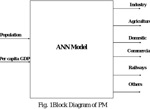
The factors like weather, temperature, number of households, number of air conditioners, oil price, economy, population, etc. are correlated with electrical energy demand. The modeling of ANN for forecasting will be difficult with large number of input data. In addition, most of these factors are required only for short-term forecasting problems. It is therefore decided to select minimum number of factors that can be effectively related to the energy demand. Among these parameters, the population growth and the per capita GDP representing the revenue and living standards of public can be associated with energy consumption [7], and therefore these two factors are chosen as inputs in the PM. The forecasted outputs are chosen as sector-wise energy demands at Industry, Agriculture, Domestic, Commercial, Railways and Others.

Population

Per capita GDP

Industry

Agriculture

Domestic

Commercial

Railways

Others

ANN Model

Fig. 1Block Diagram of PM

The input data of the per capita GDP and population, and the target data of six sector-wise energy demands form the database for developing the ANN model, which therefore contains two inputs and six outputs as shown in Fig. 1. The collected input-target data are divided into two sets: the former one, known as the training set, is employed for training the ANN, while the later one, known as testing data, is employed to assess how perfectly the ANN is modelled. Sometimes, the ANN may be poorly-modelled in such a way that it gives erroneous forecasting, which can be avoided by making the data set uniformly distributed and by changing the number of neurons in the hidden layer.

Wide range of values of input and output dataset may suppress the significance of the smaller valued data. Besides, the larger valued data may cause the activation functions of neurons to saturate. If a neuron is saturated, then it produces insignificant or no change in its output for a given change in the input. These effects influence badly the training performance and hence the collected data are normalized by Eq. (1) before using it in modeling the ANN.



 



R R R

n L

data data

L U data data

data 



  



min max

min

(1)

Wheredatan represents the normalized data

min

data anddatamaxdenotes the smallest and largest values of the data variable respectively

R

L andUR lower and upper limit for the normalized data respectively

Minimize







 

 

N

n no

i

i i n T n

O N

MSE

1 1

2

) ( ) ( 2

1

(2)

The FOA can be employed for training the ANN model. It involves representation of problem variables and the formation of a brightness function. Each firefly(F) in the FOA is defined to indicate the biases, and the connection weights between input, hidden and output layers as

] , , ,

[W_ih b_h W_ho b_o

F (3)

The FOA explores the solution space for optimal solution by maximizing a brightness function (B), which is tailored as

MSE B

Maximize

 

1 1

(4)

Fireflies usually move towards the brighter fireflies. In FOA, i-th firefly move towards j-th firefly, if j-th firefly’s brightness (B) is larger than that of i-th firefly’s, by the following expression:









) 1 ( )

(t F t A_, F t F t  rand

F_{i i ij j i}  (5)

Where Ai,jdenotes the attractiveness between i-th and j-th fireflies and is computed by









i A A E A

A min,,

2 , ,

min, , max,

,   exp  (6)

Where E_i,j is the Euclidean distance between i-th and j-th fireflies.

andiare constants

An initial population of fireflies is obtained by generating random values to every individual in the population. The brightness (B) is evaluated for each firefly. The brightness of all fireflies are compared and the fireflies with lower brightness are allowed to move towards the brighter fireflies by Eq. (5). This process represents an iteration. The iterative procedure is repeated until the number of iterations reaches the maximum number of iterations. The ANN with the connection weights obtained from best firefly in the population is ready for forecasting the future energy demand.

III. SIMULATION RESULTS

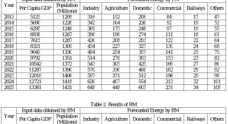
Table 1 Results of PM

Year

Input data obtained by RM Forecasted Energy by PM

Per Capita GDP Population

(Millions) Industry Agriculture Domestic Commercial Railways Others

2013 5125 1209 316 152 206 84 17 47

2014 5690 1226 342 164 226 92 19 52

2015 6295 1248 369 175 248 97 19 55

2016 6938 1267 396 196 274 111 18 61

2017 7615 1287 426 208 293 122 22 64

2018 8321 1309 454 227 327 130 24 68

2019 9049 1330 484 254 357 141 25 75

2020 9792 1351 514 278 393 153 23 82

2021 10542 1372 543 305 425 169 27 86

2022 11287 1390 570 336 466 182 29 92

2023 12018 1406 597 371 512 198 29 98

2024 12721 1418 626 407 554 213 32 101

2025 13381 1431 648 448 605 231 34 108

Table 2 Results of RM

Year

Input data obtained by RM Forecasted Energy by RM

Per Capita GDP Population

(Millions) Industry Agriculture Domestic Commercial Railways Others

2013 5125 1209 317 147 202 84 15 46

2014 5690 1226 347 165 224 97 16 51

2015 6295 1248 382 176 245 106 17 55

2016 6938 1267 418 195 279 119 20 61

2017 7615 1287 451 215 305 125 22 67

2018 8321 1309 489 233 342 142 24 73

2019 9049 1330 527 262 381 152 26 80

2020 9792 1351 556 289 426 165 27 87

2021 10542 1372 595 319 462 176 28 93

2022 11287 1390 623 348 503 192 30 100

2023 12018 1406 652 376 542 205 31 105

2024 12721 1418 674 417 596 219 33 110

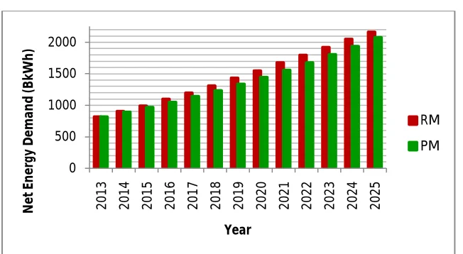
Fig. 2 Comparison of net energy demand

IV. CONCLUSION AND FUTURE WORK

Long term load forecasting estimates the future energy demand of a country and signifies a major role in allocating funds by the government for newer power plants. The sector-wise electrical energy demands of India were forecasted for the future years through considering the population and the per capita GDP as inputs of the ANN model. The FOA that mimics the flashing behavior of fireflies was employed for training the ANN model with a view of overcoming the drawbacks of the classical back-propagation training algorithm. The ANN models thus trained through FOA forecasts the sector-wise electrical energy demand. The forecasting of the PM offers lower energy demands than that of RM, and helps the policy makers for allocating lower funds for constructing new generation plants to meet the future demands. The forecasted results up to the year 2025 portrays the superiority of the developed model.

REFERENCES

1. P.E. McSharry, S. Bouwman, and G. Bloemhof, ‘Probabilistic forecasts of the magnitude and timing of peak electricity demand’, IEEE Transactions Power Systems, Vol. 20, pp. 1166-1172, 2005.

2. C.L. Hor, SJ. Watson, and S. Majithia,‘Analyzing the impact of weather variables on monthly electricity demands’, IEEE Transactions on Power Systems, Vol. 20, pp. 2078-2085, 2005.

3. Geoffrey K.F. Tso, Kelvin K.W. Yau,‘Predicting electricity energy consumption: A comparison of regression analysis, decision tree and neural networks’, Energy, Vol. 32, No. 9, pp. 1761-1768, 2007.

4. Henrique SteinherzHippert, Carlos Eduardo Pedreira, and Reinaldo Castro Souza,‘Neural networks for short-term load forecasting: a review and evaluation’, IEEE Transactions on Power Systems, Vol. 16, No.1, pp. 44-55, 2001.

5. Madasuhanmandlu and Bhavesh Kumar Chauhan,‘Load forecasting using hybrid models’, IEEE Trans. on Power Systems, Vol.26, No. 1, pp 20-29, 2011.

6. SantoshKulkarni, Sishaj P. Simon and K. Sundareswaran,‘A spiking neural network (SNN) forecast engine for short-term electrical load forecasting’, Applied Soft Computing, Vol.13, pp. 3628-3635, 2013.

7. A. Ghanhari, A. Naghavi, S.F. Ghaderi, and M. Sabaghian, ‘Artificial neural networks and regression approaches comparison for forecasting Iran's annual electricity load’, Proceeding of International Conference on Power Engineering Energy and Electrical Drives, pp. 675-679, 2009.

8. AdemAkpinar,‘Modeling and forecasting of Turkey's energy consumption using socio-economic and demographic variables’, Applied Energy, Vol. 88, No.5, pp. 1927-1939, 2011.

9. Toly Chen and Yu-Cheng Wang, ‘Long-term load forecasting by a collaborative fuzzy-neural approach’, Electrical Power and Energy Systems, Vol.43, No. 1, pp. 454-464, 2012.

10. X. S. Yang, ‘Nature-Inspired Meta-Heuristic Algorithms’, 2nd ed., Beckington, Luniver Press, 2010. 11. Data for population available at http://www.populstat.info/Asia/indiac.htm

12. Data for per capita GDP available at http://www.indexmundi.com/india/gdp_per_capita_ (ppt).html

13. India’s sector wise energy demand available at http://www.iasri.res.in/agridata/08data%5Cchapter3%5Cdb2008tb3_57.pdf