Analysis of Patterns in Data Mining
Pratik Karnik
B.E, Department of Information Technology, K.J Somaiya College of Engineering, Mumbai, India
ABSTRACT: We are living in a digital society and we are surrounded by a large amount of data. This has occurred rapidly since the advent of the computers and the internet. But lot of the data which we get is structured and the knowledge is deeply buried in this data. So we need strong tools to mine this data for its scalable analysis. Patterns form a very important aspect of this analysis and gives us great insight into the knowledge hidden in the data. This paper focuses on highlighting concepts of patterns, various efficient pattern mining methods, various patterns and their evaluations and various applications of pattern mining.
KEYWORDS: Data Mining, Pattern, Frequent Pattern Mining, Pattern Based Classification, Pattern’s Application
I. INTRODUCTION
Data Mining can be regarded as extraction of interesting patterns. Data from various sources if first preprocessed by using various methods like data normalization, dimension reduction etc. We get integrated and processed data at the end of it which could be stored in databases or data warehouses or any repository. However we are only interested in a part of it so various methods of data selection and mining are performed at this stage. After end of all this we get patterns. However patterns formed could be redundant or not so meaningful. Hence various pattern evaluation techniques are carried out like interpretation, visualization etc. Data Mining can be essentially viewed from various angles like what data is to be mined, what knowledge is to be mined, what methodologies or techniques are utilized and also where all are its applications. [1]
Patterns are a set of items, subsequences or substructures that occur together frequently in a given data set. They usually represent critical properties of data sets. Pattern discovery helps uncover various inherent regularities in the data sets. It also forms base for various data mining tasks like classifications, clustering, associations and various analysis
II. FREQUENTPATTERNSANDASSOCIATIONRULES
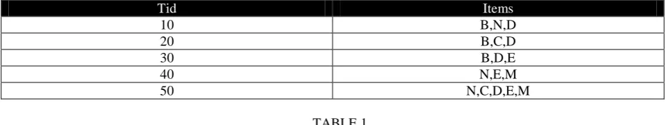
Tid Items
10 B,N,D
20 B,C,D
30 B,D,E
40 N,E,M
50 N,C,D,E,M
TABLE 1
Itemsets are set of one more of items. Absolute support of an itemset X is the frequency or the number of occurrences of an itemset X. In table 1 for item B the support is 3. Relative support is the fraction of transaction that contain X. So in this case relative support is 3/5. An itemset X is frequent of the support of X passes a minimum support threshold.
X->Y(s,c) where s is the probability that a transaction contains X and Y are there together whereas c is conditional probability that a transaction which contains X also contains Y. Thus confidence is support of X union Y divided by support of X.
However a major challenge is that in a lot of cases we end up generating too many frequent patterns, so to overcome this hurdle closed patterns and max patterns are used. X is said to be closed if X is frequent and there exist no super pattern Y with the same support as X. Closed Patterns are lossless compression of frequent patterns.[2] X is a max pattern if X is frequent and there exists no frequent super pattern Y which is a super pattern of X. However max patterns are lossy compression of frequent patterns. [3]
III. EFFECTIVEPATTERNMININGMETHODS
If there is a transaction table having transaction T1: {a1,…,a50} and T2: {a1,…,a100} the frequent itemset here is {a1,…a50}. Also all its subsets are also frequent like (a1),(a2),…,(a50),(a1,a2)…,(a1,…,a49) etc. Downward closure or the Apriori property states that any subsets of a frequent itemset must be frequent if we keep the minimal support ratio as the same.Eg. If {B,D,N} is frequent then {B,D} is also frequent. If there is an itemset A, any of its subset is infrequent, then there's no chance for A to become frequent. [4]
The Apriori Algorithm is used for mining frequent itemsets and for making various association rules. In this algorithm first the frequent itemsets are found. According to the downward closure or the apriori property a subset of a frequent itemset is also frequent. Then through various iterations frequent itemsets with cardinality from 1 to M (M-itemsets) are found. Using these frequent itemsets various association rules are generated.
Since the proposal of the famous Apriori algorithm there have been many modifications. To reduce the number of passes of database scans partitioning and dynamic itemset counting methods are used. Partitioning method ensures that the database just twice. An potentially frequent itemset in the transaction database must be frequent in at least one of its partitions. If a global database if partitioned into m partitions and if aitemset X is not frequent in any one of these m partitions then it cannot be frequent in the global database as well. [5] To shrink the size of the candidate sets direct hashing and pruning method is used. This method states that if the k-itemset is frequent then in its hashing bucket it contains several potentially frequent itemsets. So if the hash count isn’t frequent then any one of them cannot be frequent. [6]
FP Growth is a very important algorithm of the Pattern Growth Approach. In this algorithm firstly frequent single items are found. Then the database is partitioned based on such items. Then recursively more frequent patterns are generated by repeating the steps. For this a new data structure called FP Tree is used. Thus in this algorithm conditional FP trees are recursively constructed and mined until the resulting FP Tree is empty or until it contains only one path. This single path will generate all combinations of its sub paths each of which is a frequent pattern. CLOSET+ is a very effective algorithm for mining closed patterns. Itemset merging is an important method in this which suggests that if Y appears in every occurrence of X, then items in Y is merged with X. [7]
IV.EVALUATION OF PATTERNS
There are many limitations of the support – confidence framework. Pattern mining may generate a large number of rules,
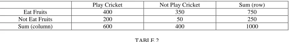
Play Cricket Not Play Cricket Sum (row)
Eat Fruits 400 350 750
Not Eat Fruits 200 50 250
Sum (column) 600 400 1000
TABLE 2
If we interpret Table 2 we can derive an association rule like playing cricket implies eating fruits as 400 out of 1000 students play cricket and eat fruits and 200 play cricket and don’t eat fruits. In this rule we get 40% support and 2/3rd
of the confidence. However if we interpret it in a different way not playing cricket and eating fruits has 35% support however they are 350 people out of 400 eating cereal which has higher confidence. This leads to an ambiguity.
To overcome these limitations of support and confidence framework other interestingness measures like lift and X2(Chi – Square) have been put forth. For two itemsets B and C, lift can be calculated as below.
As a general rule for the lift, if lift is 1 then the two items are independent. If it is greater than 1 then they are positively correlated and if it is less than 1 then they are negatively correlated. Chi-Square or X2 is another interesting measure. In this we calculate the expected value. If Chi – Square is 0 then they are independent.
If it is greater than 0 then the items are positively correlated and if it is less than zero then items are negatively correlated. However if the itemset is very large the lift and the Chi – Square may fail to give accurate results as there are many null transactions. Some measures have a property called null – invariance which means that their values do not change with the number of transactions. Following are the various null variant and null invariant measures.
The null invariance is very important and critical in massive transaction data analysis because in many transactions, the transaction set contains particular sets of rare items. These interesting measures help for a more accurate analysis of data which has a lot of null transaction which lift and X2 cant. [8]
V. MININGOFDIVERSEPATTERNS
In mining multi- level frequent patterns, items often form hierarchies. In such cases shared market level mining can be done. The lowest minimum support is used to let the high level pass down to the low level. However during analysis of rules the high level rules are filled using higher level support thresholds only. Also in mining various market level association rules a lot of redundancy can be generated as they may have hidden relationships. In this scenario if a rule can be derived from the higher level rules then the lower level rules are redundant and thus can be eliminated. Also a lot of items naturally have different support thresholds. So instead analysis each item on a specific minimal support there can be a more group based, individualistic minimum support i.e for items like luxury jewelry there can be a different minimum threshold as compared to milk etc. For mining multi- dimensional association rules usually a data cube is used.
Quantitative association rules are for actual numerical data. To mine such rules static discretization is done. However discretization may not be suitable for all cases. Where discretization is not suitable clustering on the basis of data is done. For mining rules deviation analysis is also a popular method. Deviation analysis means that instead of doing fixed interval based on certain conditions, their mean or median or any statistic measure is found. If the mean for our data is substantially deviant from the overall mean then this could be an interesting rule
Rare patterns have some rare occurring items. They have very low support but they are interesting. For rare items we should be able to set some individualized, group-based min-support threshold. That means for rare patterns, for just those items, we should set a rather low minimum support threshold, then we will be able to capture such patterns. Negative pattern means, those patterns, they are negatively correlated, that means they are unlikely happen together. When two itemsets A and B are negatively correlated, they should not be influenced by the number of null transactions. Colossal Patterns or long or large patterns are being used extensively in bioinformatics, social network analysis etc. However because of the downward closure property of frequent patterns a lot of obstacles are faced. Pattern fusion is implemented for this. In this small patterns are fused together to generate a new pattern of very large size. A colossal pattern has more core patterns than the small patterns. [9]
VI.MININGOFPATTERNSBASEDONCONSTRAINTS,SEQUENCESANDGRAPHS
If data is mined plainly on considering minimum support or minimum confidence, unnecessary number of patterns are generated and a vast number of them may not even be interesting. We can divide the constraints into two categories. First being pattern space pruning constraints and second being data space pruning constraints.
Pattern Anti-Monotonicity means that if item set X violates this constraints even though you add anything to X. If X violates this constraint then subsequent mining on X can be stopped as it is useless. Pattern Monotonicity means that if an itemset X satisfies these constraints then any of its supersets will also satisfy the same constraints. Data Anti-Monotonicity means we can prune the data space while mining. In the mining process if there is a data entry A and if that data entry doesn’t satisfy the pattern under these conditions then the data entry A cannot satisfy the pattern’s superset either. Succinct constraints are those constraints which can be enforced by directly manipulating the data. Succinctness can be used for both data and pattern space pruning. If multiple constraints need to be enforced item – ordering is required. [10]
SID SEQUENCE
10 <b(bcd)(bd)e(dg)>
20 <(be)b(cd)(bf)>
30 <(fg)(bc)(eg)dc>
40 <fh(bg)dcd>
TABLE 4
In the sequence <(fg)(bc)(eg)dc> in Table 3, the parenthesis means that they are in the same shopping basket. Each one of these may be regarded as an element. It may contain a set of items or events and these events follow one after another. However items within an element are unordered. Any substrings within a sequence are called as sub sequences and gaps are allowed in them. Sequential pattern mining algorithms should find complete set of frequent sub sequences and also should have flexibility for various user – defined constraints. The Apriori property of frequent pattern mining holds true for sequential pattern mining as well i.e if a subsequence is infrequent then any of its super sequences cannot be frequent.
GSP is a sequential mining method which is based on apriori. In this method singleton sequences are first generated from a sequence database. Then based on minimum support threshold we can eliminated items and create candidate sub sequences. So in essence GSP algorithm can be summarized as scanning the database to find length X frequent sequences and then generating length (X+1) candidate sets using apriori recursively until no further frequent sequence or candidates can be found out. [11]
Sequential pattern mining can also be done using a pattern growth space algorithm called Prefix Span. Prefix means anything in the front and if it is frequent then it is known as frequent prefix and same goes for suffixes. For a given sequence, there will be a set of prefixes and a set of suffixes. In this method first length – 1 sequential patterns are found. If they are frequent they are called as length – 1 sequential pattern. Later using divide and conquer the whole search space is divided so as to mine the projected database. However largely redundant sub sequences are generated but they are largely redundant with the original string. But real physical prediction is not done, instead pseudo projection is done. Major advantages of Prefix Span is that no candidate sub sequences are generated and the projected database keeps on reducing. [12]
When the database is held in the main memory, pseudo projection is very effective as there is no need for physically copying suffixes and also only pointer is needed to the sequence and we get an offset of the suffix at the end. But if it doesn’t fit in memory then physical projection is preferred. An integration of physical and pseudo projection is most effective and also swapping to pseudo projection is needed when data fits in the memory.
CloSpan is an algorithm for mining closed sequential patterns. Closed sequential patterns mean that of there exists no super pattern A super and if A super and A have same support then A is a closed sequential pattern. We can mine all sequential patterns and then determine which ones are closed. However it is not very efficient and so directly mining closed sequential patterns is necessary as it will not only reduce the number of redundant patterns to be generated but it will also attain the same expressive power as it is a lossless compression. If an itemset A is a superset of A1, then A is closed if and only of two project databases have the same size. [13]
Constraint based sequential pattern mining is similar to constraint based frequent pattern mining other than the fact than sequence is of significance in the former. There are also some timing based constraints in sequential mining which enforces conditions about minimum and max time spans between two elements etc. In episode pattern mining there are mainly two types of episodes namely serial episodes when a particular element occurs before another or parallel episodes when the two elements are in sync.
subgraph is said to be frequent if and only if all of its subgraphs are frequent. A candidate size (X+1) edge/ vertex subgraph is generated if its corresponding two X edge/vertex subgraphs are frequent. This method is an iterative mining process. Firstly candidates are generated then they are pruned then support is counted and on its basis various candidates are eliminated and this happens iteratively. [14]
An m-edge frequent graph may contain 2 raised to m subgraphs, thus it becomes difficult to handle so many graphs. To avoid this combinatorial explosion problem, closed sequential patterns are mined. A frequent graph G is closed if there exists no super graph of g that carries the same support as G. Mining of closed graph patterns is considered as lossless compression even though it does not contain non-closed graphs. [15]
In many databases there are a lot of interesting useful graphs and if one searches based on the structures one may want to build a structure based index like graph index. If there is an index structure and if a graph query is done in such a database then results can be fetched really efficiently. Indexing frequent substructures is usually preferred as if they are indexed then overall search is done. For this the minimum threshold is decided by using size increasing support threshold which means that smaller the size lower is the minimum support threshold.
FIGURE 1
Thus to maintain limited size structure for effectiveness, size increasing minimum support threshold is used to index graphs. Apart from indexing frequent substructures, there is a need for indexing discriminative substructures also. Discriminative substructures mean that if there are already some substructures in the index structure then new subgraphs are obtained and even they are frequent, however if they are similar to the current one or covered by the current one then it is not advisable to select this as an index structure. This reduces index size by an order of magnitude. Discriminative substructures can be compared to people having different skillsets in a group. If those skills aren’t present in the research group then a new person is selected, however if the new person’s skill can be covered by people in the group then that person become less in demand and demand for person with exceptional skill rises.
VII. PATTERNBASEDCLASSIFICATION
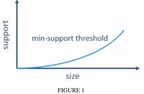
Classification is also known as supervised learning. The gist of classification is that given a set of training instances then various classification methods can be invoked which involve machine learning, construction of models and after this prediction models are obtained and once validated they can be used for real classification or to predict new cases.
FIGURE 2
Support Vector Machine is one of the most popular classification method in which maximum margin is found so that difference cases can be partitioned in a clear way. In decision tree method different conditions are found which can go through different branches. In network simulation, a simulation of human brain which has various layers and this network is trained for quality classification. Bayesian Network method which is based on Bayesian Induction formulae are found which can be used as classifiers and when a new scenario comes network is analysed for right classes.
Pattern based classification means use of frequent and discriminative patterns for effective classification. If patterns are effectively mined they can be used as good classifiers and this help classification process. Pattern based classification is an integration of frequent pattern mining and classification.
FIGURE 3
Pattern based classification is a feature construction process. Through this type of classification multiple features can be constructed together to get higher order which can be discriminative as well as compact. Through pattern based classification complex features like graphs, sequences and semi and unstructured data can also be constructed. With help of pattern based classification, complicated things can be transformed into a set of clear discriminative patterns. In a dataset patterns or association rules can be found out so as to construct good classification models.
In classification based on association (CBA) firstly high confidence and high support association rules are mined. Then these rules are sorted and are ranked in descending order of confidence and support. Then first rule which matches the
TRAINING
INSTANCES
TEST
INSTANCES
PREDICTION
MODEL
MODEL
LEARNING
POSITIVE
NEGATIVE
FREQUENT
PATTERN MINING
PATTERN BASED
test case is applied or else the default rule is applied. This method is very effective as exploring high confident associations among multiple attributes may overcome constraints caused by classifiers that take into account only one attribute at a given point of time. [17]
In classification based on multiple association rules (CMAR), rule pruning is done whenever a rule is inserted into the tree. In this method given two rules A1 and A2, if antecedent of A1 is more general than that of A2 and confidence of A1 is greater than or equal to confidence of A2 then A2 is prunes. Also rules are pruned for the rules whose rule antecedents and class labels are not positively correlated as per the chi-square test. The classification is then carried out based on the pruned rules. If only one rule satisfies a tuple A then class label of the rule is assigned. If a rule set B satisfies tuple X then B is divided into various groups on the basis of class labels. Then using chi – square measure the strongest group of rules are found out and X is assigned the class label of the strongest group. [18]
In Discriminative frequent pattern classification initially discriminative frequent patterns are mined as high quality features and then they are used as classifiers for further analysis Feature construction is firstly done by frequent item mining. Then feature selection is carried out in which discriminative features are selected and redundant or closely correlated features are removed. Using these features model learning is done by applying a general classifier to build a classification model.
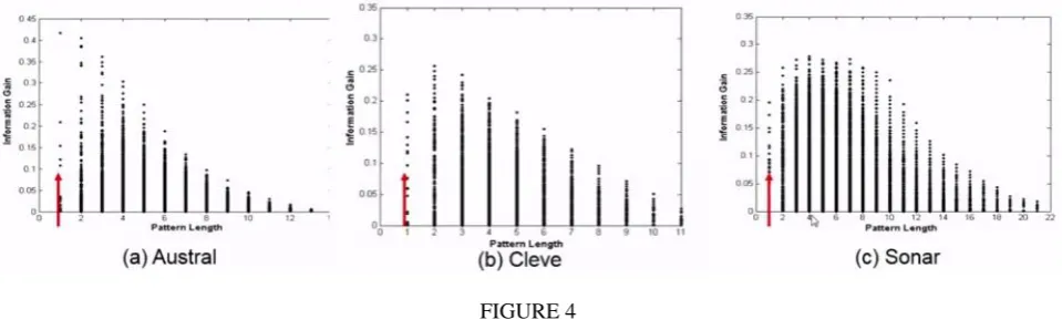
FIGURE 4
X-itemsets are more often more informative than single feature itemsets in classification as longer patterns carry lot more of information gain as seen in Figure 4. The discriminative power of X-itemsets where X is between 10 and 1 usually is higher than the single features. Information gain bound monotonically increases with pattern frequency.
In direct mining of discriminative patterns a set of training instances and features are taken as input and feature selection is iteratively performed on them and the feature with the highest discriminative power is selected and instances covered by the selected feature are removed. It is implemented as an integration of branch and bound search with FP growth mining. Training instances can also be eliminated iteratively in implementation and thus FP tree can be reduced. In this methodology the discriminative power or information gain of a low frequency pattern is bounded at the upper level by a small value. Then when FPGrowth mining is performed the most discrimination itemset and its information gain is recorded. Also before the conditional FP-tree is developed, an estimation of upper bound of information gain is made. If the upper bound value is less than information gain of the most discriminative itemset then then FP tree and its subsequent trees are not considered. [19]
VIII. ADVANCEDPATTERNMINING
constructed and each single word is treated as an individual one and modelling is then done. After that words are combined into the same topic and topics are visualized with phrases. Lastly a prior bag of words model is also used where firstly phrase mining and construction of phrases is done and then those constraints are imposed on bag of words model.
In simultaneously inferring phrases and topics, Bigram Topic Model is used which is a probabilistic generative model that conditions on previous word and topic when drawing next word. Also Topical N Gram model is preferred which is a probabilistic model that generates words in a textual border by creating n grams by concatenating successive bigrams. In phrase discovering LDA each sentence is viewed as a time series of words and it is stated that the topic changes periodically and each word is drawn based on previous a words and current phrase topic. [20]
In Post Topic Modelling Phrase Construction topic modelling on the basis of back off words in document is firstly done. In TurboTopics method construction of phases is done based on the same topic label i.e firstly Latent Dirichlet Allocated is performed on the corpus to assign each token a topic label. Then the adjacent unigrams with the same topic label are merged. This merging is done till all significant adjacent unigrams are merged. In KERT method, phase construction is done as a post process to LDA. In this method frequent pattern mining is done on each topic and then phase ranking is done based on various criteria. In KERT bag of words model is first run and topic labels are assigned to each token. Then using frequent pattern mining, candidate key phrases are extracted in each topic and these candidate key phrases are ranked in terms of popularity, discriminativeness, concordance and completeness.[21] In First Phrase Mining then Topic Modelling, frequent contiguous pattern mining is done to obtain candidate phrases and their counts. Then agglomerative merging of adjacent unigrams is done This segments each document into a bag of phrases. This is later on passed as input to PhraseLDA that constrains all words in a phrase to each sharing the same latent topic.[22] The simultaneously inferring phrases and topics is an integrated complex model and phrase quality and topic inference rely on each other but it is slow and overfitting. In simultaneously inferring phrases and topics phrase quality relies on topic labels for unigrams and can be fast. In First Phrase Mining then Topic Modelling, topic inference relies on correct segmentation of documents and can be fast as well.
Mining precise frequent patterns in stream data is unrealistic as we cannot even store them in a compressed form. However approximate answers are often sufficient for pattern analysis. For this Lossy Counting Algorithm whose main ideology is not to keep items with very low support count. In this algorithm the stream is divided into buckets. Then we count buckers and at bucket boundary all counters are decreased by 1. Then we keep on adding buckets like this. The frequency count error is less than the number of buckets in this method and we get an output of items with frequency counts exceeding the difference between the support threshold and error threshold multiplied by stream length. [23]
In Spatial frequent patterns and association rules if A implies B, here A and B are sets of spatial and non-spatial predicates like topological relations, spatial orientations, distances etc. In progressive refinement in mining spatial associations the rough patterns are mined first and then they are refined to see exactly what pattern they are. Refinement saves a lot of processing time. Mining of spatial associations can be regarded as a two-step process in whose first step a rough spatial computation as filter is done using Minimum Bounding Rectangle or R-tree for rough estimates. In second step detailed spatial algorithm is implemented as refinement in which refinement is applied to only those objects which have passed rough spatial i.e which are not less than minimum support. In case of sparse data, clustering is done to find reference points and then multiple interleaved periods are detected by Fourier Transformation and auto-correlation. Semantic Trajectory is a trajectory that carries semantics. Meaningful sequential patterns can be found by observing semantic consistencies, spatial compactness and temporal continuity. In Semantic Trajectory Pattern Mining firstly coarse patterns that satisfy the semantic and temporal constraints are mined. Then dense and compact clusters are detected in high dimensional space. Later on the coarse patterns are split into fined grained ones to meet spatial constraint. So first semantic meaningful trajectories are found then refined using more spatiotemporal information thereby finding their sub patterns. [24]
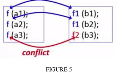
and Paste Bugs are an important category of bugs. To mine forget to change bugs, sequential pattern mining is done in which build sequence database from source code, then sequential pattern mining is carried out and mismatched identifiers and bugs are found out.
FIGURE 5
To build a sequence database, each statement is mapped to a number and each component is tokenized. Then the program is mapped to a long sequence. In this method max gap is constrained and neighbouring copy pasted segments are combined repeatedly. Then names are identified which cannot be mapped to the corresponding ones. If unchanged ratio is between 0 and threshold then it is reported as a bug as a conflict is found here as seen in Figure 6.
For ensuring privacy of the data statistical distortion can be done by using randomized algorithms in which either independent attribute perturbation is done or dependent attribute perturbation. MASK is a method in which each bit is flipped with a probability and that probability is tuned carefully to achieve acceptable average privacy and good accuracy. In cut and paste operator, uniform randomization is done to protect data privacy. In this each existing item is replaced with a new item which is not present in the original transaction. [25]
IX.CONCLUSION
The paper gives a comprehensive idea about various patterns and association rules along with effective pattern mining methods. Along with this various ways of evaluation of patterns is put along with analysis of methods of mining diverse patterns as well as analysis of pattern mining based on constraints, graphs and sequences. Lastly classification based on pattern and some applications and advanced pattern mining concepts are put forth.
In the future as data increases and more and more unstructured data comes up, a lot of challenges will be faced. However pattern mining emerges as a promising tool for analysis of trends and coming up with effective analytical solutions to various problems
X. RESULTS
Table 1 gives an illustration for describing the concepts of support, confidence and association rules. Table 2 provides an example of ambiguous cases arising in association rules. Table 3 provides data about various interestingness measures. Table 4 demonstrates an examples of sequences in data mining.
REFERENCES
[1] Jiawei Han, Micheline Kamber and Jian Pei, “Data Mining: Concepts and Techniques”, Morgan Kaufmann, 3rd edition, 2011 [2] N. Pasquier, Y. Bastide, R. Taouil and L. Lakhal, “Discovering frequent closed itemsets for association rules” in Proc of ICDT 1999 [3] R. J Bayardo, “Efficiently mining long patterns from databases”, in Proc. Of SIGMOD 1998
[4] R. Agrawal and R. Srikant, “Fast Algorithms for Mining Association Rules”, in VLDB 1994
[5] A. Savasere, E. Omiecinski and S. Navathe, “An Efficient Algorithm for Mining Association Rules in Large Databases” in VLDB 1995 [6] J. Park, M. Chen and P. Yu, “An effective hash based algorithm for mining association rules” in SIGMOD 1995.
[7] J. Han, J. Pei and Y. Yin, “Mining frequent patterns without candidate generation”, in SIGMOD 2000
[8] P.-N. Tan, V. Kumar and J.Srivastava, “Selecting the Right Interestingness Measure for Association Patterns” in KDD 2002 [9] F. Zhu, X. Yan, P.S. Yu and H. Cheng, “Mining Colossal Frequent Patterns by Core Pattern Fusion”, in ICDE 2007 [10] G. Grahne, L. Lakshmanan and X. Wang, “Efficient mining of constrained correlated sets”, in ICDE 2001
[11] R. Srikant and R. Agrawal, “Mining sequential patterns : Generalizations and performance improvements”, EDBT 1996
[12] J. Pei, J. Han, B. Mortazavi –Asl, J. Wang, H. Pinto, Q. Chen, U. Dayal and M.-C. Hsu,” Mining sequential patterns by pattern – growth : The PrefixSpan Approach”, in IEEE TKDE,16(10) 2004
[13] X. Yan, J. Jan and R.Afshar, “CloSpan : Mining Closed Sequential Patterns in Large Datasets”, in SDM 2003
[14] A. Inokuchi, T. Washio an H. Motoda, “An apriori based algorithm for mining frequent substructures from graph data”, in PKDD 2000 [15] X. Yan and J. Han, “Closegraph : Mining closed frequent graph patterns”, in KDD 2003
[16] F. Zhu, Q. Qu, D. Lo, X. Yan, J.Han and P.S. Yu, “Mining Top K Large Structural Patterns in a Massive Network”, in VLDB 2011 [17] B. Liu, W. Hsu and Y. Ma, “Integrating Classification and Association Rule Mining”, in KDD 1998
[18] W. Li, J. Han and J.Pei, “CMAR : Accurate and Efficient Classification based on Multiple Class Association Rules”, in ICDM 2001 [19] H. Cheng, X. Yan, J. Han and P.S. Yu, “Direct Discriminative Pattern Mining for Effective Classfication”, in ICDE 2008
[20] X. Wang, A, McCallum, X. Wei, “Topical N grams : Phrase and topic discovery with an application to information retrieval”, in ICDM 2007 [21] M. Danilesvsky, C. Wang, N. Desai, J. Guo, J. Han, “Automatic Construction and Ranking of Topical Keyphrases on Collection of Short Documents”, in SDM 2014
[22] A. El-Kishky, Y. Song, C. Wang, C.R. Voss, J. Han, “Scalable Topical Phrase Mining from Text Corpora”, in VLDB 2015 [23] G. Manku and R. Motwani, “Approximate Frequency Counts Over Data Streams”, in VLDB 2002
[24] C. Zhang, J. Han, L. Shou, J. Lu, T. La Porta, “Splitter : Mining fine grained sequential patterns in semantic trajectories”, in VLDB 2014 [25] S. Rizvi and J. Haritsa, “Maintaining data privacy in association rule mining”, in VLDB 2002
BIOGRAPHY