Joe Celko's Data and Databases: Concepts in Practice
by Joe Celko ISBN: 1558604324
Morgan Kaufmann Publishers © 1999, 382 pages
A "big picture" look at database design and programming for all levels of developers.
Table of Contents Colleague Comments
Back Cover
Synopsis by Dean Andrews
In this book, outspoken database magazine columnist Joe Celko waxes philosophic about fundamental concepts in database design and
development. He points out misconceptions and plain ol' mistakes commonly made while creating databases including mathematical calculation errors, inappropriate key field choices, date representation goofs and more. Celko also points out the quirks in SQL itself. A detailed table-of-contents will quickly route you to your area of interest.
Table of Contents
Joe Celko’s Data and Databases: Concepts in Practice - 4
Preface - 6
Chapter 1
- The Nature of Data
- 13Chapter 2
- Entities, Attributes, Values, and Relationships
- 23 Chapter 3- Data Structures
- 31Chapter 4
- Relational Tables
- 49 Chapter 5- Access Structures
- 69 Chapter 6- Numeric Data
- 84Chapter 7
- Character String Data
- 92 Chapter 8- Logic and Databases
- 104 Chapter 9- Temporal Data
- 123 Chapter 10- Textual Data
- 131 Chapter 11- Exotic Data
- 135Chapter 12
- Scales and Measurements
- 146 Chapter 13- Missing Data
- 151Chapter 15
- Check Digits
- 163Chapter 16
- The Basic Relational Model
- 178 Chapter 17- Keys
- 188Chapter 18
- Different Relational Models
- 202 Chapter 19- Basic Relational Operations
- 205Chapter 20
- Transactions and Concurrency Control
- 207 Chapter 21- Functional Dependencies
- 214Chapter 22
- Normalization
- 217 Chapter 23- Denormalization
- 238 Chapter 24- Metadata
- 252 References - 258Back Cover
Do you need an introductory book on data and databases? If the book is by Joe Celko, the answer is yes. Data & Databases: Concepts in Practice is the first introduction to relational database technology written especially for practicing IT professionals. If you work mostly outside the database world, this book will ground you in the concepts and overall framework you must master if your data-intensive projects are to be successful. If you’re already an experienced database programmer, administrator, analyst, or user, it will let you take a step back from your work and examine the founding principles on which you rely every day -- helping you work smarter, faster, and problem-free.
Whatever your field or level of expertise, Data & Databases offers you the depth and breadth of vision for which Celko is famous. No one knows the topic as well as he, and no one conveys this knowledge as clearly, as effectively -- or as engagingly. Filled with absorbing war stories and no-holds-barred commentary, this is a book you’ll pick up again and again, both for the information it holds and for the distinctive style that marks it as genuine Celko.
Features:
• Supports its extensive conceptual information with example code and other practical illustrations.
• Explains fundamental issues such as the nature of data and data modeling and moves to more specific technical questions such as scales, measurements, and encoding.
• Offers fresh, engaging approaches to basic and not-so-basic issues of database programming, including data entities, relationships and values, data structures, set operations, numeric data, character string data, logical data and operations, and missing data.
• Covers the conceptual foundations of modern RDBMS technology, making it an ideal choice for students.
Joe Celko is a noted consultant, lecturer, writer, and teacher, whose column in
Intelligent Enterprise has won several Reader’s Choice Awards. He is well known for his ten years of service on the ANSI SQL standards committee, his dependable help on the DBMS CompuServe Forum, and, of course, his war stories, which provide real-world insight into SQL programming.
Joe Celko’s Data and Databases: Concepts in
Practice
Joe Celko
Senior Editor: Diane D. Cerra
Director of Production and Manufacturing: Yonie Overton Production Editor: Cheri Palmer
Editorial Coordinator: Belinda Breyer
Cover and Text Design: Side by Side Studios Cover and Text Series Design: ThoughtHouse, Inc. Copyeditor: Ken DellaPenta
Proofreader: Jennifer McClain Composition: Nancy Logan Illustration: Cherie Plumlee Indexer: Ty Koontz
Printer: Courier Corporation
Designations used by companies to distinquish their products are often claimed as trademarks or registered trademarks. In all instances where Morgan Kaufmann Publishers is aware of a claim, the product names appear in initial capital or all capital letters. Readers, however, should contact the appropriate companies for more complete information regarding trademarks and registration.
Morgan Kaufmann Publishers
Editorial and Sales Office
340 Pine Street, Sixth Floor San Francisco, CA 94104-3205 USA
Telephone: 415/392-2665 Facsimile: 415-982-2665 E-mail: [email protected] www: http://www.mkp.com Order toll free: 800/745-7323
Printed in the United States of America
To my father, Joseph Celko Sr., and to my daughters, Takoga Stonerock and Amanda Pattarozzi
Preface
Overview
This book is a collection of ideas about the nature of data and databases. Some of the material has appeared in different forms in my regular columns in the computer trade and academic press, on CompuServe forum groups, on the Internet, and over beers at conferences for several years. Some of it is new to this volume.
This book is not a complete, formal text about any particular database theory and will not be too mathematical to read easily. Its purpose is to provide foundations and philosophy to the working programmer so that they can understand what they do for a living in greater depth. The topic of each chapter could be a book in itself and usually has been.
This book is supposed to make you think and give you things to think about. Hopefully, it succeeds.
Thanks to my magazine columns in DBMS, Database Programming & Design, Intelligent
Enterprise, and other publications over the years, I have become the apologist for
ANSI/ISO standard SQL. However, this is not an SQL book per se. It is more oriented toward the philosophy and foundations of data and databases than toward programming tips and techniques. However, I try to use the ANSI/ISO SQL-92 standard language for examples whenever possible, occasionally extending it when I have to invent a notation for some purpose.
If you need a book on the SQL-92 language, you should get a copy of Understanding the
New SQL, by Jim Melton and Alan Simon (Melton and Simon 1993). Jim’s other book,
Understanding SQL’s Stored Procedures (Melton 1998), covers the procedural language
that was added to the SQL-92 standard in 1996.
If you want to get SQL tips and techniques, buy a copy of my other book, SQL for Smarties
(Celko 1995), and then see if you learned to use them with a copy of SQL Puzzles &
Answers (Celko 1997).
Organization of the Book
The book is organized into nested, numbered sections arranged by topic. If you have a problem and want to look up a possible solution now, you can go to the index or table of contents and thumb to the right section. Feel free to highlight the parts you need and to write notes in the margins.
Corrections and Future Editions
I will be glad to receive corrections, comments, and other suggestions for future editions of this book. Send your ideas to
Joe Celko
235 Carter Avenue Atlanta, GA 30317-3303
email: [email protected] website: www.celko.com
or contact me through the publisher. You could see your name in print!
Acknowledgments
I’d like to thank Diane Cerra of Morgan Kaufmann and the many people from CompuServe forum sessions and personal letters and emails. I’d also like to thank all the members of the ANSI X3H2 Database Standards Committee, past and present.
Chapter 1:
The Nature of Data
Where is the wisdom? Lost in the knowledge. Where is the knowledge? Lost in the information. —T. S. Eliot
Where is the information? Lost in the data. Where is the data?
Lost in the #@%&! database! — Joe Celko
Overview
So I am not the poet that T. S. Eliot is, but he probably never wrote a computer program in his life. However, I agree with his point about wisdom and information. And if he knew the distinction between data and information, I like to think that he would have agreed with mine.
I would like to define “data,” without becoming too formal yet, as facts that can be represented with measurements using scales or with formal symbol systems within the context of a formal model. The model is supposed to represent something called “the real world” in such a way that changes in the facts of “the real world” are reflected by changes in the database. I will start referring to “the real world” as “the reality” for a model from now on.
1.2 Information versus Wisdom
Wisdom does not come out of the database or out of the information in a mechanical fashion. It is the insight that a person has to make from information to handle totally new situations. I teach data and information processing; I don’t teach wisdom. However, I can say a few remarks about the improper use of data that comes from bad reasoning.
1.2.1 Innumeracy
Innumeracy is a term coined by John Allen Paulos in his 1990 best-seller of the same
title. It refers to the inability to do simple mathematical reasoning to detect bad data, or bad reasoning. Having data in your database is not the same thing as knowing what to do with it. In an article in Computerworld, Roger L. Kaydoes a very nice job of giving
examples of this problem in the computer field (Kay 1994).
1.2.2 Bad Math
Bruce Henstell (1994) stated in the Los Angeles Times: “When running a mile, a 132 pound woman will burn between 90 to 95 calories but a 175 pound man will drop 125 calories. The reason seems to be evolution. In the dim pre-history, food was hard to come by and every calorie has to be conserved—particularly if a woman was to conceive and bear a child; a successful pregnancy requires about 80,000 calories. So women should keep exercising, but if they want to lose weight, calorie count is still the way to go.”
Calories are a measure of the energy produced by oxidizing food. In the case of a person, calorie consumption depends on the amount of oxygen they breathe and the body material available to be oxidized.
Let’s figure out how many calories per pound of human flesh the men and women in this article were burning: (95 calories/132 pounds) = .71 calories per pound of woman and (125 calories/175 pounds) = .71 calories per pound of man. Gee, there is no difference at all! Based on these figures, human flesh consumes calories at a constant rate when it exercises regardless of gender. This does not support the hypothesis that women have a harder time losing fat through exercise than men, but just the opposite. If anything, this shows that reporters cannot do simple math.
Another example is the work of Professor James P. Allen of Northridge University and Professor David Heer of USC. In late 1991, they independently found out that the 1990 census for Los Angeles was wrong. The census showed a rise in Black Hispanics in South Central Los Angeles from 17,000 in 1980 to almost 60,000 in 1990. But the total number of Black citizens in Los Angeles has been dropping for years as they move out to the suburbs (Stewart 1994).
Furthermore, the overwhelming source of the Latino population is Mexico and then Central America, which have almost no Black population. In short, the apparent growth of Black Hispanics did not match the known facts.
not adjusted for inflation, he would still have lost!
1.3 Models versus Reality
A model is not reality, but a reduced and simplified version of it. A model that was more complex than the thing it attempts to model would be less than useless. The term “the real world” means something a bit different than what you would intuitively think. Yes, physical reality is one “real world,” but this term also includes a database of information about the fictional worlds in Star Trek,the “what if” scenarios in a spreadsheet or discrete simulation program, and other abstractions that have no physical forms. The main characteristic of “the real world” is to provide an authority against which to check the validity of the database model.
A good model reflects the important parts of its reality and has predictive value. A model without predictive value is a formal game and not of interest to us.
The predictive value does not have to be absolutely accurate. Realistically, Chaos Theory shows us that a model cannot ever be 100% predictive for any system with enough structure to be interesting and has a feedback loop.
1.3.1 Errors in Models
Statisticians classify experimental errors as Type I and Type II. A Type I error is
accepting as false something that is true. A Type II error is accepting as true something that is false. These are very handy concepts for database people, too.
The classic Type I database error is the installation in concrete of bad data, accompanied by the inability or unwillingness of the system to correct the error in the face of the truth. My favorite example of this is a classic science fiction short story written as a series of letters between a book club member and the billing computer. The human has returned an unordered copy of Kidnapped by Robert Louis Stevenson and wants it credited to his account.
When he does not pay, the book club computer turns him over to the police computer, which promptly charges him with kidnapping Robert Louis Stevenson. When he objects, the police computer investigates, and the charge is amended to kidnapping and murder, since Robert Louis Stevenson is dead. At the end of the story, he gets his refund credit and letter of apology after his execution.
While exaggerated, the story hits all too close to home for anyone who has fought a false billing in a system that has no provision for clearing out false data.
The following example of a Type II error involves some speculation on my part. Several years ago a major credit card company began to offer cards in a new designer color with higher limits to their better customers. But if you wanted to keep your old card, you could have two accounts. Not such a bad option, since you could use one card for business and one for personal expenses.
They needed to create new account records in their database (file system?) for these new cards. The solution was obvious and simple: copy the existing data from the old account without the balances into the new account and add a field to flag the color of the card to get a unique identifier on the new accounts.
some were for the new card without any prior history, and some were for the new “two accounts” option.
One of the fields was the date of first membership. The company thinks that this date is very important since they use it in their advertising. They also think that if you do not use a card for a long period of time (one year), they should drop your membership. They have a program that looks at each account and mails out a form letter to these unused
accounts as it removes them from the database.
The brand new accounts were fine. The replacement accounts were fine. But the members who picked the “two card” option were a bit distressed. The only date that the system had to use as “date of last card usage” was the date that the original account was opened. This was almost always more than one year, since you needed a good credit history with the company to get offered the new card.
Before the shiny new cards had been printed and mailed out, the customers were getting drop letters on their new accounts. The switchboard in customer service looked like a Christmas tree. This is a Type II error—accepting as true the falsehood that the last usage date was the same as the acquisition date of the credit card.
1.3.2 Assumptions about Reality
The purpose of separating the formal model and the reality it models is to first
acknowledge that we cannot capture everything about reality, so we pick a subset of the reality and map it onto formal operations that we can handle.
This assumes that we can know our reality, fit it into a formal model, and appeal to it when the formal model fails or needs to be changed.
This is an article of faith. In the case of physical reality, you can be sure that there are no logical contradictions or the universe would not exist. However, that does not mean that you have full access to all the information in it. In a constructed reality, there might well be logical contradictions or vague information. Just look at any judicial system that has been subjected to careful analysis for examples of absurd, inconsistent behavior.
But as any mathematician knows, you have to start somewhere and with some set of primitive concepts to be able to build any model.
Chapter 2:
Entities, Attributes, Values, and
Relationships
Perfection is finally attained not when there is no longer anything to add but when there is no longer anything to take away.
—Antoine de Saint Exupery
Overview
What primitives should we use to build a database? The smaller the set of primitives, the better a mathematician feels. A smaller set of things to do is also better for an
they are very well defined for us.
Entities, attributes, values, and relationships are the components of a relational model. They are all represented as tables made of rows, which are made of columns in SQL and the relational model, but their semantics are very different. As an aside, when I teach an SQL class, I often have to stress that a table is made of rows, and not rows and columns; rows are made of columns. Many businesspeople who are learning the relational model think that it is a kind of spreadsheet, and this is not the case. A spreadsheet is made up of rows and columns, which have equal status and meaning in that family of tools. The cells of a spreadsheet can store data or programs; a table stores only data and constraints on the data. The spreadsheet is active, and the relational table is passive.
2.1 Entities
An entity can be a concrete object in its reality, such as a person or thing, or it can be a relationship among objects in its reality, such as a marriage, which can handled as if it were an object. It is not obvious that some information should always be modeled as an entity, an attribute, or a relationship. But at least in SQL you will have a table for each class of entity, and each row will represent one instance of that class.
2.1.1 Entities as Objects
Broadly speaking, objects are passive and are acted upon in the model. Their attributes are changed by processes outside of themselves. Properly speaking, each row in an object table should correspond to a “thing” in the database’s reality, but not always uniquely. It is more convenient to handle a bowl of rice as a single thing instead of giving a part number to each grain.
Clearly, people are unique objects in physical reality. But if the same physical person is modeled in a database that represents a company, they can have several roles. They can be an employee, a stockholder, or a customer.
But this can be broken down further. As an employee, they can hold particular positions that have different attributes and powers; the boss can fire the mail clerk, but the mail clerk cannot fire the boss. As a stockholder, they can hold different classes of stock, which have different attributes and powers. As a customer, they might get special discounts from being a customer-employee.
The question is, Should the database model the reality of a single person or model the roles they play? Most databases would model reality based on roles because they take actions based on roles rather than based on individuals. For example, they send
paychecks to employees and dividend checks to stockholders. For legal reasons, they do not want to send a single check that mixes both roles.
It might be nice to have a table of people with all their addresses in it, so that you would be able to do a change of address operation only once for the people with multiple roles. Lack of this table is a nuisance, but not a disaster. The worst you will do is create redundant work and perhaps get the database out of synch with the reality. The real problems can come when people with multiple roles have conflicting powers and actions within the database. This means that the model was wrong.
A relationship is a way of tying objects together to get new information that exists apart from the particular objects. The problem is that the relationship is often represented by a token of some sort in the reality.
A marriage is a relationship between two people in a particular legal system, and its token is the marriage license. A bearer bond is also a legal relationship where either party is a lawful individual (i.e., people, corporations, or other legal creations with such rights and powers).
If you burn a marriage license, you are still married; you have to burn your spouse instead (generally frowned upon) or divorce them. The divorce is the legal procedure to drop the marriage relationship. If you burn a bearer bond, you have destroyed the relationship. A marriage license is a token that identifies and names the relationship. A bearer bond is a token that contains or is itself the relationship.
You have serious problems when a table improperly models a relationship and its entities at the same time. We will discuss this problem in section 2.5.1.
2.2 Attributes
Attributes belong to entities and define them. Leibniz even went so far as to say that an
entity is the sum of all its attributes. SQL agrees with this statement and models attributes as columns in the rows of tables that can assume values.
You should assume that you cannot ever show in a table all the attributes that an entity has in its reality. You simply want the important ones, where “important” is defined as those attributes needed by the model to do its work.
2.3 Values
A value belongs to an attribute. The particular value for a particular attribute is drawn from a domain or has a datatype. There are several schools of thought on domains, datatypes, and values, but the two major schools are the following:
1. Datatypes and domains are both sets of values in the database. They are both finite sets because all models are finite. The datatype differs by having operators in the hardware or software so the database user does not have to do all that work. A domain is built on a subset of a datatype, which inherits some or all of its operators from the original datatype and restrictions, but now the database can have user-defined operators on the domain.
2. A domain is a finite or infinite set of values with operators that exists in the database’s reality. A datatype is a subset of a domain supported by the computer the database resides on. The database approximates a domain with a subset of a datatype, which inherits some or all of its operators from the original datatype and other restrictions and operators given to it by the database designer.
Unfortunately, SQL-92 has a CREATEDOMAIN statement in its data declaration language (DDL) that refers to the approximation, so I will refer to database domains and reality domains.
definitions give a rule that determines if a value is in the domain or not. You have seen both of these approaches in elementary set theory in the list and rule notations for defining a set. For example, the finite set of positive even numbers less than 16 can be defined by either
A = {2, 4, 6, 8, 10, 12, 14}
or
B = {i : (MOD(i, 2) = 0) AND (i > 0) AND (i < 16)}
Defining the infinite set of all positive even numbers requires an ellipsis in the list notation, but the rule set notation simply drops restrictions, thus:
C = {2, 4, 6, 8, 10, 12, 14, . . .}
D = {i : MOD(i, 2) = 0}
While this distinction can be subtle, an intentional definition lets you move your model from one database to another much more easily. For example, if you have a machine that can handle integer datatypes that range up to (216) bits, then it is conceptually easy to move the database to a machine that can handle integer datatypes that range up to (232) bits because they are just two different approximations of the infinite domain of integers in the reality. In an extensional approach, they would be seen as two different datatypes without a reference to the reality.
For an abstract model of a DBMS, I accept a countably infinite set as complete if I can define it with a membership test algorithm that returns TRUE or FALSE in a finite amount of time for any element. For example, any integer can be tested for evenness in one step, so I have no trouble here.
But this breaks down when I have a test that takes an infinite amount of time, or where I cannot tell if something is an element of the set without generating all the previous elements. You can look up examples of these and other such misbehaved sets in a good math book (fractal sets, the (3 * n + 1) problem, generator functions without a closed form, and so forth).
The (3 * n + 1) problem is known as Ulam’s conjecture, Syracuse’s problem, Kakutani’s problem, and Hasse’s algorithm in the literature, and it can be shown by this procedure (see Lagarias 1985 for details).
FUNCTION ThreeN (i INTEGER IN, j INTEGER IN) RETURNS INTEGER; LANGUAGE SQL
BEGIN
DECLARE k INTEGER; SET k = 0;
WHILE k <= j LOOP
SET k = k + 1; IF i IN (1, 2, 4)
THEN ThreeN((i / 2), k) ELSE ThreeN((3 * i + 1), k); END LOOP;
RETURN 1 -- answer is True END WHILE;
We are trying to construct a subset of all the integers that test true according to the rules defined in this procedure. If the number is even, then divide it by two and repeat the procedure on that result. If the number is odd, then multiply it by three, add one, and repeat the procedure on that result. You keep repeating the procedure until it is reduced to one.
For example, if you start with 7, you get the sequence (7, 22, 11, 34, 17, 52, 26, 13, 40, 20, 10, 5, 16, 8, 4, 2, 1, . . .), and seven is a member of the set. Bet that took longer than you thought!
As a programming tip, observe that when a result becomes 1, 2, or 4, the procedure hangs in a loop, endlessly repeating that sequence. This could be a nonterminating program, if we are not careful!
An integer, i, is an element of the set K(j) when i fails to arrive at one on or before j
iterations. For example, 7 is a member of K(17). By simply picking larger and larger values of j, you can set the range so high that any computer will break. If the j parameter is dropped completely, it is not known if there are numbers that never arrive at one. Or to put it another way, is this set really the set of all integers?
Well, nobody knows the last time I looked. I have to qualify that statement this way, because in my lifetime I have seen solutions to the four-color map theorem and Fermat’s Last theorem proven. But Gödel proved that there are always statements in logic that cannot be proven to be TRUE or FALSE, regardless of the amount of time or the number of axioms you are given.
2.4 Relationships
Relationships exist among entities. We have already talked about entities as relationships and how the line is not clear when you create a model.
2.5 ER Modeling
In 1976 Peter Chen invented entity-relationship (ER) modeling as a database design technique. The original diagrams used a box for an entity, a diamond for a relationship, and lines to connect them. The simplicity of the diagrams used in this method have made it the most popular database design technique in use today. The original method was very minimal, so other people have added other details and symbols to the basic diagram.
There are several problems with ER modeling:
I feel that people should spend more time actually designing data elements, as you can see from the number of chapters in this book devoted to data.
2. Although there can be more than one normalized schema from a single set of constraints, entities, and relationships, ER tools generate only one diagram. Once you have begun a diagram, you are committed to one schema design.
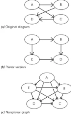
3. The diagram generated by ER tools tends to be a planar graph. That means that there are no crossed lines required to connect the boxes and lines. The fact that a graph has crossed lines does not make it nonplanar; it might be rearranged to avoid the crossed lines without changes to the connections (see Fig. 2.1).
Fig. 2.1
A planar graph can also be subject to another graph theory result called the “four-color map theorem,” which says that you only need four “four-colors to “four-color a planar map so that no two regions with a common border have the same color.
4. ER diagrams cannot express certain constraints or relationships. For example, in the versions that use only straight lines between entities for relationships, you cannot easily express an n-ary relationship (n > 2).
Furthermore, you cannot show constraint among the attributes within a table. For example, you cannot show the rule that “An employee must be at least 18 years of age” with a constraint of the form CHECK((hiredate-birthdate)>=INTERVAL 18YEARS).
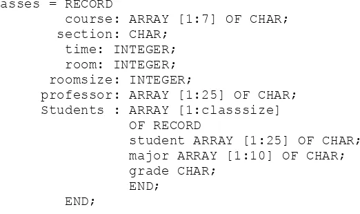
As an example of the possibility of different schemas for the same problem, consider a database of horse racing information. Horses are clearly physical objects, and we need information about them if we are going to calculate a betting system. This modeling decision could lead to a table that looks like this:
CREATE TABLE Horses
What is wrong with this table? First of all, this table is not normalized. Consider what happens when a middle manager named 'JerryRivers' decides that he needs to change his name to 'GeraldoRiviera' to get minority employment preferences. This change will have to be done once in the emp_name column and n times in the
boss_name column of each of his immediate subordinates. One of the defining
characteristics of a normalized database is that one fact appears in one place, one time, and one way in the database.
Next, when you see 'JerryRivers' in the emp_name column, it is a value for the name attribute of a Personnel entity. When you see 'JerryRivers' in the boss_name column, it is a relationship in the company hierarchy. In graph theory, you would say that this table has information on both the nodes and the edges of the tree structure in it.
There should be a separate table for the employees (nodes), which contains only
employee data, and another table for the organizational chart (edges), which contains only the organizational relationships among the personnel.
2.5 ER Modeling
In 1976 Peter Chen invented entity-relationship (ER) modeling as a database design technique. The original diagrams used a box for an entity, a diamond for a relationship, and lines to connect them. The simplicity of the diagrams used in this method have made it the most popular database design technique in use today. The original method was very minimal, so other people have added other details and symbols to the basic diagram.
There are several problems with ER modeling:
1. ER does not spend much time on attributes. The names of the columns in a table are usually just shown inside the entity box, without datatypes. Some products will indicate which column(s) are the primary keys of the table. Even fewer will use another notation on the column names to show the foreign keys.
I feel that people should spend more time actually designing data elements, as you can see from the number of chapters in this book devoted to data.
2. Although there can be more than one normalized schema from a single set of constraints, entities, and relationships, ER tools generate only one diagram. Once you have begun a diagram, you are committed to one schema design.
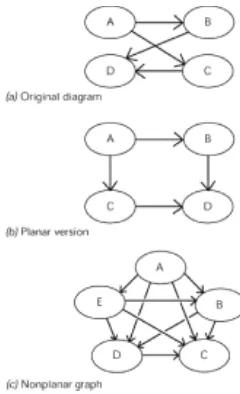
Fig. 2.1
A planar graph can also be subject to another graph theory result called the “four-color map theorem,” which says that you only need four “four-colors to “four-color a planar map so that no two regions with a common border have the same color.
4. ER diagrams cannot express certain constraints or relationships. For example, in the versions that use only straight lines between entities for relationships, you cannot easily express an n-ary relationship (n > 2).
Furthermore, you cannot show constraint among the attributes within a table. For example, you cannot show the rule that “An employee must be at least 18 years of age” with a constraint of the form CHECK((hiredate-birthdate)>=INTERVAL 18YEARS).
As an example of the possibility of different schemas for the same problem, consider a database of horse racing information. Horses are clearly physical objects, and we need information about them if we are going to calculate a betting system. This modeling decision could lead to a table that looks like this:
CREATE TABLE Horses
(horsename CHAR(30) NOT NULL, track CHAR(30) NOT NULL,
race INTEGER NOT NULL CHECK (race > 0), racedate DATE NOT NULL,
position INTEGER NOT NULL CHECK (position > 0), finish CHAR(10) NOT NULL
CHECK (finish IN ('win', 'place', 'show', 'ran', 'scratch')), PRIMARY KEY (horsename, track, race, racedate));
There should be a separate table for the employees (nodes), which contains only
employee data, and another table for the organizational chart (edges), which contains only the organizational relationships among the personnel.
2.6 Semantic Methods
Another approach to database design that was invented in the 1970s is based on semantics instead of graphs. There are several different versions of this basic approach, such as NIAM (Natural-language Information Analysis Method), BRM (Binary
Relationship Modeling), ORM (Object-Role Modeling), and FORM (Formal Object-Role Modeling). The main proponent of ORM is Terry Halpin, and I strongly recommend getting his book (Halpin 1995) for details of the method. What I do not recommend is using the diagrams in his method. In addition to diagrams, his method includes the use of simplified English sentences to express relationships. These formal sentences can then be processed and used to generate several schemas in a mechanical way.
Most of the sentences are structured as subject-verb-object, but the important thing is that the objects are assigned a role in the sentence. For example, the fact that “Joe Celko wrote Data and Databases for Morgan Kaufmann Publishers” can be amended to read “AUTHOR: Joe Celko wrote BOOK: ‘Data and Databases’ for PUBLISHER: Morgan Kaufmann,” which gives us the higher level, more abstract sentence that “Authors write books for publishers” as a final result, with the implication that there are many authors, books, and publishers involved. Broadly speaking, objects and entities become the subjects and objects of the sentences, relationships become verbs, and the constraints become prepositional phrases.
A major advantage of the semantic methods is that a client can check the simple
sentences for validity easily. An ER diagram, on the other hand, is not easily checked. One diagram looks as valid as another, and it is hard for a user to focus on one fact in the diagram.
Chapter 3:
Data Structures
Overview
Data structures hold data without regard to what the data is. The difference between a physical and an abstract model of a data structure is important, but often gets blurred when discussing them.
Each data structure has certain properties and operations that can be done on it, regardless of what is stored in it. Here are the basics, with informal definitions.
Data structures are important because they are the basis for many of the implementation details of real databases, for data modeling, and for relational operations, since tables are multisets.
3.1 Sets
use the term “empty set.”
The expression “same kind of thing” is a bit vague, but it is important. In a database, the rows of a table have to be instances of the same entity; that is, a Personnel table is made up of rows that represent individual employees. However, a grouped table built from the Personnel table, say, by grouping of departments, is not the same kind of element. In the grouped table, the rows are aggregates and not individuals. Departmental data is a different level of abstraction and cannot be mixed with individual data.
The basic set operations are the following:
• Membership:is or is not a member of a particular set. The symbol is This operation says how elements are related to a set. An element either ∈.
• Containment: One set A contains another set B if all the elements of B are also
elements of A. B is called a subset of A. This includes the case where A and B are the same set, but if there are elements of A that are not in B, then the relationship is called
proper containment. The symbol is ⊂; if you need to show “contains or equal to,” a
horizontal bar can be placed under the symbol (⊆).
It is important to note that the empty set is not a proper subset of every set. If A is a subset of B, the containment is proper if and only if there exists an element b in B such that b is not in A. Since every set contains itself, the empty set is a subset of the empty set. But this is not proper containment, so the empty set is not a proper subset of every set.
• Union:sets. The symbol is The union of two sets is a single new set that contains all the elements in both ∪. The formal mathematical definition is
∀x: x∈ A ∨x∈ B ⇒
x∈ (A ∪ B)
• Intersection: elements common to both sets. The symbol is The intersection of two sets is a single new set that contains all the ∩. The formal mathematical definition is
∀x: x ∈ A ∧x∈ B ⇒
x∈ A ∩ B
•
Difference:elements from A that are not in B. The symbol is a minus sign. The difference of two sets A and B is a single new set that contains
∀x: x∈ A
∧ ¬ (x ∈) B ⇒
x∈ (A – B)
•
Partition:that The partition of a set A divides the set into subsets, A1, A2, . . . , An, such
∪ A [i] = A
∧∩ A [i] = Ø
A multiset (also called a bag) is a collection of elements of the same type with duplicates of the elements in it. There is no ordering of the elements in a multiset, and we still have the empty set. Multisets have the same operations as sets, but with extensions to allow for handling the duplicates.
Multisets are the basis for SQL, while sets are the basis for Dr. Codd’s relational model.
The basic multiset operations are derived from set operations, but have extensions to handle duplicates:
• Membership:∈. In addition to a value, an element also has a degree of duplication, which tells you An element either is or is not a member of a particular set. The symbol is the number of times it appears in the multiset.
Everyone agrees that the degree of duplication of an element can be greater than zero. However, there is some debate as to whether the degree of duplication can be zero, to show that an element is not a member of a multiset. Nobody has proposed using a negative degree of duplication, but I do not know if there are any reasons not to do so, other than the fact that it does not make any intuitive sense.
For the rest of this discussion, let me introduce a notation for finding the degree of duplication of an element in a set:
dod(<multiset>, <element>) = <integer value>
• Reduction:converts it into a set. In SQL, this is the effect of using a This operation removes redundant duplicates from the multiset and SELECTDISTINCT clause.
For the rest of this discussion, let me introduce a notation for the reduction of a set:
red(<multiset>)
•
Containment: One multiset A contains another multiset B if
1.red(A) ⊂ red(B)
2.∀x∈ B: dod(A, x) = dod(B, x)
This definition includes the case where A and B are the same multiset, but if there are elements of A that are not in B, then the relationship is called proper containment.
•
Union:elements in both multisets. A more formal definition is The union of two multisets is a single new multiset that contains all the
∀x: x∈ A ∨ x∈ B ⇒
x∈ A ∪ B
∧
The degree of duplication in the union is the sum of the degree of duplication from both tables.
•
Intersection:the elements common to both multisets. The intersection of two multisets is a single new multiset that contains all
∀x: x∈ A ∧x∈ B ⇒
x∈ A ∩ B
∧
dod(A ∩ B, x) = ABS (dod(A, x) – dod(BB, x))
The degree of duplication in the intersection is based on the idea that you match pairs from each set in the intersection.
• Difference:contains elements from A that are not in B after pairs are matched from the two The difference of two multisets A and B is a single new multiset that multisets. More formally:
∀x: x∈ A
∧ ¬ (x∈) B ⇒
x∈ (A – B)
∧ dod((A – B), x) = (dod(A, x) – dod(B, x))
• Partition:. , An, such that their multiset union is the original set and their multiset intersection is The partition of a multiset A divides it into a collection of multisets, A1, A2, . . empty.
Because sets are so important in the relational model, we will return to them in Chapter 4
and go into more details.
3.3 Simple Sequential Files
Simple files are a linear sequence of identically structured records. There is a unique first record in the file. All the records have a unique successor except the unique last record. Records with identical content are differentiated by their position in the file. All processing is done with the current record.
In short, a simple sequential file is a multiset with an ordering added. In a computer system, these data structures are punch cards or magnetic tape files; in SQL this is the basis for CURSORs. The basic operations are the following:
• Open the file: This makes the data available. In some systems, it also positions a
read-write head on the first record of the file. In others, such as CURSORs in SQL, the read-write head is positioned just before the first record of the file. This makes a difference in the logic for processing the file.
•
Fetch a record: This changes the current record and comes in several different flavors:
1.Fetch next: The successor of the current record becomes the new current record.
3.Fetch last: The last record becomes the new current record.
4.Fetch previous:record. The predecessor of the current record becomes the new current
5.Fetch absolute: The nth record becomes the new current record.
6.Fetch relative:current record. The record n positions from the current record becomes the new
There is some debate as to how to handle a fetch absolute or a fetch relative command that would position the read-write head before the first record or after the last record. One argument is that the current record should become the first or last record, respectively; another opinion is that an error condition should be raised.
In many older simple file systems and CURSOR implementations, only fetch next is available. The reason was obvious with punch card systems; you cannot “rewind” a punch card reader like a magnetic tape drive. The reason that early CURSOR
implementations had only fetch next is not so obvious, but had to do with the disposal of records as they were fetched to save disk storage space.
•
Close the file: This removes the file from the system.
•
Insert a record:record becomes its successor. The new record becomes the current record, and the former current
•
Update a record:not change position. Values within the current record are changed. The read-write does
• Delete a record:becomes the current record. If the current record was the last record of the file, the read-This removes a record from the file. The successor of the current record write head is positioned just past the end of the file.
3.4 Lists
A list is a sequence of elements, each of which can be either a scalar value called an
atom or another list; the definition is recursive. The way that a list is usually displayed is as a comma-separated list within parentheses, as for example, ((Smith, John), (Jones, Ed)).
A list has only a few basic operations from which all other functions are constructed. The head() function returns the first element of a list, and the tail() function returns the rest of it. A constructor function builds a new list from a pair of lists, one for the head and one for the tail of the new list.
Lists are important in their own right, and the LISP programming language is the most common way to manipulate lists. However, we are interested in lists in databases because they can represent complex structures in a fast and compact form and are the basis for many indexing methods.
List programming languages also teach people to think recursively, since that is usually the best way to write even simple list procedures. As an example of a list function, consider Member(), which determines if a particular atom is in a list. It looks like this in pseudocode:
BOOLEAN PROCEDURE Member (a ATOM IN, l LIST IN) IF l IS ATOMIC
THEN RETURN (a = l) ELSE IF member(a, hd(l)) THEN RETURN TRUE
ELSE RETURN member(a, tl(l));
The predicate <list>ISATOMIC returns TRUE if the list expression is an atom.
3.5 Arrays
Arrays are collections of elements accessed by using indexes. This terminology is
unfortunate because the “index” of an array is a simple integer list that locates a value within the array, and not the index used on a file to speed up access. Another term taken from mathematics for “index” is “subscript,” and that term should be favored to avoid confusion.
Arrays appear in most procedural languages and are usually represented as a subscript list after the name of the array. They are usually implemented as contiguous storage locations in host languages, but linked lists can also be used. The elements of an array can be records or scalars. This is useful in a database because it gives us a structure in the host language into which we can put rows from a query and access them in a simple fashion.
3.6 Graphs
Graphs are made up of nodes connected by edges. They are the most general abstract
data structure and have many different types. We do not need any of the more complicated types of graphs in a database and can simply define an edge as a relationship between two nodes. The relationship is usually thought of in terms of a traversal from one node to another along an edge.
The two types of graphs that are useful to us are directed and undirected graphs. An edge in a directed graph can be traversed in only one direction; an edge in an undirected graph can be traversed in both directions. If I were to use a graph to represent the traffic patterns in a town, the one-way streets would be directed edges and the two-way streets would be undirected edges. However, a graph is never shown with both types of edges— instead, an undirected graph can be simulated in a directed graph by having all edges of the form (a,b) and (b,a) in the graph.
database, so we can model all of those things, too.
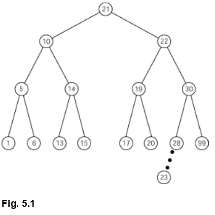
3.7 Trees
A tree is a special case of a graph. There are several equivalent definitions, but the most useful ones are the following:
•
A tree is a graph with no cycles. The reason that this definition is useful to a database user is that circular references can cause a lot of problems within a database.
• A tree is made up of a node, called a parent, that points to zero or more other nodes, its children, or to another tree. This definition is recursive and therefore very compact, but another advantage is that this definition leads to a nested-sets model of
hierarchies.
Trees are the basis for indexing methods used in databases. The important operations on a tree are locating subtrees and finding paths when we are using them as an index. Searching is made easier by having rules to insert values into the tree. We will discuss this when we get to indexes.
Relational Philosopher
The creator of the relational model talks about his never-ending crusade.
Interviewing Dr. Edgar F. Codd about databases is a bit like interviewing Einstein about nuclear physics. Only no one has ever called the irascible Codd a saint. In place of Einstein’s publications on the theory of relativity, you have Codd’s ground-breaking 1970 paper on relational theory, which proposed a rigorous model for database management that offered the beguiling simplicity of the rows and columns of tables. But there was more to it than that. Codd’s work was firmly grounded in the mathematical theory of relations of arbitrary degree and the predicate logic first formulated by the ancient Greeks. Moreover, it was a complete package that handled mapping the real world to data structures as well as manipulating that data—that is, it included a specification for a normal form for database relations and the concept of a universal data sublanguage.
Almost as important to its success, Codd’s relational theory had Codd backing it. The former World War II Royal Air Force pilot made sure word got out from his IBM research lab to the world at large. In those early years he had to struggle against the political forces aligned behind IBM’s strategic database product, IMS, and came to work each day “wondering who was going to stab me in the back next.” Codd parried often and well, although observers say some of the blows Codd returned over the years were imagined or had even been struck for Codd’s own relational cause.
Codd won the great database debate and, with it, such laurels as the 1981 ACM (Association for Computing Machinery) Turing Award “for fundamental and continuing contributions to the theory and practice of database management systems.”
supported the existential quantifier. He said, “Well I get some funny questions, but this is the first time I’ve been asked about support for existential philosophy.” So right there, I knew that he didn’t know a damn thing about predicate logic.
DBMS: I guess for him it wasn’t an an [sic] intuitive leap to connect predicate logic to the management of data. But you made that leap somehow?
CODD: I felt that it was a natural thing to do. I did my studies in logic and
mathematics and it occurred to me as a natural thing for queries. Then it occurred to me—and I can’t say why ideas occurred to me, but they keep doing so, and I’m not short of them even now, I can tell you—why limit it to queries? Why not take it to database management in general? Some work had already gone on in special-purpose query systems that were software on top of and separate from a database management system. It occurred to me that predicate logic could be applied to maintaining the logical integrity of the data.
DBMS: Can you quickly try to give DBMS readers a grasp for existential quantifiers in particular and predicate logic in general in case they don’t have one?
CODD: Sometimes I use this example: Statement A is strictly stronger in the logical sense than statement B if A logically implies B, but B does not logically imply A. Clearly, given a set of things and a property P that may or may not hold for each member of the set, the statement “P holds for all members of the set” is stronger than the statement “P holds for some members of the set.” In predicate logic the former statement involves the universal quantifier, while the latter involves the existential quantifier.
Mathematicians are looking for generality, for results that apply to all numbers of some kind, like all integers, or all real numbers, or all complex numbers so that they don’t have to keep making up theorems. That’s the beauty of something like Pythagoras’ theorem from ancient Greek times. It still applies to all right angle triangles, whether you’re using it for surveying or for navigating a ship. How the Greeks got on to the things they did—there was no need for surveying, or things of that nature, at that time—is amazing to me.
Excerpt from DBMS interview with Edgar F. Codd, “Relational Philosopher.” DBMS, Dec. 1990, pgs. 34–36. Reprinted with permission from Intelligent Enterprise Magazine.
Copyright © 1990 by Miller Freeman, Inc. All rights reserved. This and related articles can be found on www.intelligententerprise.com.
Chapter 4:
Relational Tables
Overview
SQL is classified as a set-oriented language, but in truth it did not have a full collection of classic set operations until the SQL-92 standard, and even then actual products were slow to implement them.
We discussed the formal properties of multisets (or bags, to use a term I find less attractive), which included
2.
A multiset has no ordering to its elements.
3.
A multiset may have duplicates in the collection.
A relational table has more properties than its simple data structure. It is far too easy for a beginner SQL programmer to think that a table is a file, a row is a record, and a column is a field. This is not true at all.
A table can exist only within a database schema, where it is related to the other tables and schema objects. A file exists in its own right and has no relationship to another file as far as the file system is concerned.
A file is passive storage whose structure is defined by the program that reads it. That is, I can read the same file in, say, Fortran several different ways in different programs by using different FORMAT statements. A file (particularly in Fortran, Cobol, and other older 3GL languages) is very concerned with the physical representation of the data in storage.
A table never exposes the physical representation of the data to the host program using it. In fact, one part of the SQL-92 standard deals with how to convert the SQL datatypes into host language datatypes, so the same table can be used by any of several standard programming languages.
A table has constraints that control the values that it can hold, while a file must depend on application programs to restrict its content. The structure of the table is part of the schema.
The rows of a table are all identical in structure and can be referenced only by name. The records in a file are referenced by position within the file and can have varying structure. Examples of changing record structures include arrays of different sizes and dimensions in Fortran, use of the OCCURS clause in Cobol, the variant records in Pascal, and struct declaration in C.
Perhaps more importantly, a row in a properly designed table models a member of a collection of things of the same kind. The notion of “things of the same kind” is a bit vague when you try to formalize it, but it means that the table is a set and whatever property applies to one row should apply to all rows.
The notion of kind also applies to the level of aggregation and abstraction used. For example, a Personnel table is a set of employees. A department is made up of
employees, but it is not an aggregation of the employees. You can talk about the salary of an employee, but it makes no sense to talk about the salary of a department. A department has a budget allocation that is related to the salaries. At another level, you can talk about the average salary of an employee within a department.
This is not always true with files. For example, imagine a company with two types of customers, wholesale and retail. A file might include fields for one type of customer that do not apply to the other and inform the program about the differences with flags in the records. In a proper database schema, you would need a table for each kind of customer, although you might have a single table for the data common to each kind.
only be accessed by their name; the database system locates them physically.
A column can have constraints that restrict the values it can contain in addition to its basic datatype; a field is limited only by the datatype that the host program is expecting. This lack of constraints has led to such things as 'LATER' being used in a field that is supposed to hold a date value.
A field can be complex and have its own internal structure, which is exposed to the application program. The most common example of this is Cobol, where a field is made up of subfields. For example, a date has year, month, and day as separate fields within it. There is nothing in Cobol per se to prevent a program from changing the day of the month to 99 at the subfield level, even though the result is an invalid date at the field level.
A properly designed column is always a scalar value. The term “scalar” means that the value is taken from a scale of some sort. It measures one attribute and only one attribute. We will discuss scales and measurement theory later in the book. In SQL, a date is a datatype in its own right, and that prevents you from constructing an invalid value.
4.1 Subsets
The name pretty much describes the concept—a subset is a set constructed from the elements of another set. A proper subset is defined as not including all the elements of the original set.
We already discussed the symbols used in set theory for proper and improper subsets. The most important property of a subset is that it is still a set. SQL does not have an explicit subset operator for its tables, but almost every single table query produces a subset. The SELECTDISTINCT option in a query will remove the redundant duplicate rows.
Standard SQL has never had an operator to compare tables against each other for equality or containment. Several college textbooks on relational databases mention a CONTAINS predicate, which does not exist in SQL-89 or SQL-92. This predicate existed in the original System R, IBM’s first experimental SQL system, but it was dropped from later SQL implementations because of the expense of running it.
4.2 Union
The union of two sets yields a new set whose elements are in one, the other, or both of the original sets. This assumes that the elements in the original sets were of the same kind, so that the result set makes sense. That is, I cannot union a set of numbers and a set of vegetables and get a meaningful result.
SQL-86 introduced the UNION and the UNIONALL operators to handle the multiset problems. The UNION is the classic set operator applied to two table expressions with the same structure. It removes duplicate rows from the final result; the UNIONALL operator leaves them in place.
columns of REAL numbers, and both give a location on a map. The UNION makes no sense unless you convert one system of coordinates into the other.
In SQL-89, the columns of the result set did not have names, but you could reference them by a position number. This position number could only be used in a few places because the syntax would make it impossible to tell the difference between a column number and an integer. For example, does 1 + 1 mean “double the value in column one,” “increment column one,” or the value two?
In SQL-92, the use of position numbers is “deprecated,” a term in the standards business that means that it is still in the language in this standard, but that the next version of the standard will remove it. The columns of the result set do not have names unless you explicitly give the columns names with an AS clause.
(SELECT a, b, c FROM Foo) UNION [ALL]
(SELECT x, y, z FROM Bar) AS Foobar(c1, c2, c3)
In practice, actual SQL products have resolved the missing names problem several different ways: use the names in the first table of the operation, use the names in the last table of the operation, or make up system-generated names.
4.3 Intersection
The intersection of two sets yields a new set whose elements are in both of the original sets. This assumes that the datatypes of the elements in the original sets were the same, so that the result set makes sense.
If the intersection is empty, then the sets are called disjoint. If the intersection is not empty, then the sets have what is called a proper overlap.
SQL-92 introduced the INTERSECT and the INTERSECTALL operators to handle the multiset problems. The INTERSECT is the classic set operator applied to two table expressions with the same structure. It removes duplicate rows from the final result; the INTERSECTALL operator matches identical rows from one table to their duplicates in the second table. To be more precise, if R is a row that appears in both tables T1 and T2, and there are m duplicates of R in T1 and n duplicates of R in T2, where m > 0 and n > 0, then the INTERSECTALL result table of T1 and T2 contains the minimum of m and n duplicates of R.
4.4 Set Difference
The set difference of two sets, shown with a minus sign in set theory, yields a subset of the first set, whose elements exclude the elements of the second set—for example, the set of all employees except those on the bowling team. Again, redundant duplicates are removed if EXCEPT is specified.
If the EXCEPTALL operator is specified, then the number of duplicates of row R that the result table can contain is the maximum of (m – n) and 0.
A partitioning of a set divides the set into subsets such that
1.
No subset is empty.
2.
The intersection of any combination of the subsets is empty.
3.
The union of all the subsets is the original set.
In English, this is like slicing a pizza. You might have noticed, however, that there are many ways to slice a pizza.
4.5.1 Groups
The GROUPBY operator in SQL is a bit hard to explain because it looks like a partition, but it is not. The SQL engine goes to the GROUPBY clause and builds a partitioned working table in which each partition has the same values in the grouping columns. NULLs are grouped together, even though they cannot be equal to each other by convention.
Each subset in the grouped table is then reduced to a single row that must have only group characteristics. This result set is made up of a new kind of element, namely, summary information, and it is not related to the original table anymore.
The working table is then passed to the HAVINGclause, if any, and rows that do not meet the criteria given in the HAVING clause are removed.
4.5.2 Relational Division
Relational division was one of the original eight relational operators defined by Dr. Codd. It is different from the other seven because it is not a primitive operator, but can be defined in terms of the other operators. The idea is that given one table with columns (a,b), called the dividend, and a second table with column (a), called the divisor, we can get a result table with column (b), called the quotient. The values of (b) that we are seeking are those that have all the values of (a) in the divisor associated with them. To make this more concrete, if you have a table of pilots and the planes they are certified to fly called PilotSkills, and a table with the planes in our hangar, when you divide the PilotSkills table by the hangar table, you get the names of the pilots who can fly every plane in the hangar.
As an analog to integer division, there is the possibility of a remainder (i.e., pilots who have certifications for planes that are not in the hangar leave those extra planes as a remainder). But if you want to draw an analogy between dividing by an empty set and division by zero, you have to be careful depending on the query you used. You can get all the pilots, even if they do not fly any planes at all, or you can get an empty result set (see my other book, SQL for Smarties, for more details).
The idea of Codd’s original division operator was that it would be an inverse of the CROSS JOIN or Cartesian product. That is, if you did a CROSSJOIN on the divisor and the quotient, you would get the rows found in the dividend table.
1.
Remove duplicates automatically.
2.
Allow duplicates.
3.
Reduce duplicates to a count of the members in the class.
4.6.1 Allow Duplicates
This is the SQL solution. The rationale for allowing duplicate rows was best defined by David Beech in an internal paper for the ANSI X3H2 committee and again in a letter to
Datamation (Beech 1989). This is now referred to as the “cat food argument” in the
literature. The name is taken from the example of a cash register slip, where you find several rows, each of which lists a can of cat food at the same price. To quote from the original article:
For example, the row ‘cat food 0.39’ could appear three times [on a supermarket checkout receipt] with a significance that would not escape many shoppers. . . . At the level of abstraction at which it is useful to record the information, there are no value components that distinguish the objects. What the relational model does is force people to lower the level of abstraction, often inventing meaningless values to be inserted in an extra column whose purpose is to show what we knew already, that the cans of cat food are distinct.
All cans of cat food are interchangeable, so they have no natural unique identifier. The alternative of tagging every single can of cat food in the database with a unique machine-readable identifier preprinted on the can or keyed in at the register is not only expensive and time-consuming, but it adds no real information to the data model. In the real world, you collect the data as it comes in on the cash register slip, and consolidate it when you debit the count of cans of cat food in the inventory table. The cans of cat food are considered equivalent, but they are not identical.
You also encounter this situation when you do a projection on a table and the result is made up of nonkey columns. Counting and grouping queries also implies that duplicate rows exist in a “separate but equal” way; that is, you treat them as a class or a multiset. Let’s make this more concrete with the following two tables:
CREATE TABLE Personnel
(emp CHAR(30) NOT NULL PRIMARY KEY, dept CHAR(8) NOT NULL);
CREATE TABLE Automobiles (owner CHAR(30) NOT NULL, tag CHAR(10) NOT NULL, color CHAR(5) NOT NULL, PRIMARY KEY(owner, tag));
You can use these tables to answer the question: “Do more employees in the accounting department than in the advertising department drive red cars?” You can answer this quickly with the following query:
SELECT dept, COUNT(*)
WHERE owner = emp AND color = 'red'
AND dept IN ('acct', 'advert') GROUP BY dept;
Try to do this without knowing that people can own more than one car and that a
department has more than one employee! Duplicate values occur in both projections and joins on these tables.
4.6.2 Disallow Duplicates
This is Chris Date’s relational model. Date has written several articles on the removal of duplicates (e.g., Date 1990, 1994). Date’s model says that values are drawn from a particular domain, which is a set of scalars. This means that when a column defined on the color domain uses the value “red”, it is using “red” in the domain and it occurs once. There might be many occurrences of references to “red” or “3” or “1996-12-25”, but they are pointing to the only red, the only integer three, and the only Christmas Day in 1996. Domains are based on an identity concept and disallow duplicate values. This is the same argument that mathematicians get into about pure numbers.
Date’s example of the problems of duplicates uses the following two tables:
Parts
SupParts
pno pname
supno
pno
p1 screw
s1
p1
p1 screw
s1
p1
p1 screw
s1
p2
p2 screw
and then attempts to write SQL to comply with the criterion “List the part numbers of screws or parts that come from supplier s1 (or both).” He produces a dozen different queries that are all different, and all produce a different number of answers. For example, if you assume that a part must have one supplier, you can write
SELECT P.pno
FROM Parts AS P, SupParts AS SP WHERE (SP.supno = 's1'
which gives the result:
pno
p1
p1
p1
p1
p1
p1 9 duplicates
p1
p1
p1
p2
p2 3 duplicates
p2
However, the more direct query that translates an OR into a UNION would give
SELECT pno FROM Parts
WHERE pname = 'screw' UNION
SELECT pno FROM SupParts WHERE supno = 's1';
pno
p1
p2
The real problem