Proceedings of Recent Advances in Natural Language Processing, pages 270–275, 270
Lexical Quantile-Based Text Complexity Measure
Maksim Eremeev AITHEA
Konstantin Vorontsov National University of Science
and Technology MISIS [email protected]
Abstract
This paper introduces a new approach to esti-mating the text document complexity. Com-mon readability indices are based on average length of sentences and words. In contrast to these methods, we propose to count the num-ber of rare words occurring abnormally often in the document. We use the reference corpus of texts and the quantile approach in order to determine what words are rare, and what fre-quencies are abnormal. We construct a general text complexity model, which can be adjusted for the specific task, and introduce two special models. The experimental design is based on a set of thematically similar pairs of Wikipedia articles, labeled using crowdsourcing. The ex-periments demonstrate the competitiveness of the proposed approach.
1 Introduction
Automated text complexity measurement tools have been proposed in order to help teachers to select textbooks that correspond to the students’ comprehension level and publishers to explore whether their articles are readable. Thus, plenty of readability indexes were developed. Mea-sures like Automated Readability Index (Senter and Smith,1967),Flesch-Kincaid readability tests (Flesh,1951), SMOG index (McLaughlin,1969), Gunning fog (Gunning,1952) and etc. use heuris-tics based on simple statisheuris-tics such as total number of words, mean number of words per sentence, to-tal number of sentences or even number of sylla-bles to evaluate how complex given text is. By combining these statistics with different weight-ing factors, readability indexes assign the given document a complexity score, which is, in most cases, the approximate representation of the US grade level needed to comprehend the text. For in-stance, an Automated Readability Index (ARI) has the following form for the documentd:
ARI(d) = 4.71× c
w+ 0.5× w
s −21.43 (1) wherecrefers to the total number of letters in the documentd,wis the total number of words ands denotes the total number of sentences ind.
Since readability indexes rely on a few basic factors, precise assessment requires aggregation
of many scores. Thus, Coh-Metrix-PORT tool
(Aluisio et al., 2010) includes more than 50 dif-ferent indexes for Portuguese language. The tool is based on Coh-Metrix (Graesser et al., 2004) principles to estimate complexity and cohesion not only for explicit text, but for the mental represen-tation of the document.
Readability indexes are interpretable and easy to implement. However, the great number of con-stants tuned specifically for the English language texts, lack of the semantics consideration and tai-loring to the US grade level system restrains the number of possible applications.
As for the non-English languages, several lex-ical and morphologlex-ical features for Italian to solve text simplification problem were presented (Brunato et al., 2015), supervised approach in readability estimations was introduced (vor der Brck et al.,2008) and the complexity estimations for legal documents in Russian were explored (Dzmitryieva,2017).
based on their relevance (Koutrika et al., 2015). The more specific terms document contains, and the more rare they are, the more complex the doc-ument is. To formalize this consideration, we esti-mate the complexity of each term in the document and then aggregate them to get the complete doc-ument complexity score. We use Wikipedia as a reference collectionof moderately complex texts in order to determine what term frequencies are abnormal.
In section 2 we describe quantile approach to estimate the single term complexity. We present highly flexible general model in section 3 and models in subsections 3.1 and 3.2. The way of evaluating the proposed methods is introduced in section 4 and the experiments result are provided in section 5.
2 Single Term Complexity Estimation
Reference collection: Let D denote a reference collection. Let documentd ∈Dconsist of terms t1, t2, . . . tnd, wherendrefers to the length of
doc-umentd. Each term can be either a single word or a key phrase.
Quantile approach: In general case each term can occur in different complexity states, which may depend on a position in text or context sur-rounding the term. Each complexity state of the term ti standing in position iis described with a term complexity scorec(ti). Consider a complex-ity scores empirical distribution for each term over the reference collection. Assume that termtiisin complex stateif its complexityc(ti)in current text positioniis greater thanγ-quantileCγ(ti) of the distribution overc(ti), whereγ is a hyperparam-eter, responsible for the complexity level. There-fore, when estimating complexity score of the doc-ument, we countc(ti)only for termsti which are in the complex state, defined by theγ parameter.
For instance, c(ti) can be a constant, which means all terms have identical complexity, or can be set equal to 0 if it occurs in the reference collec-tion and 1 otherwise. In this case, we count new terms (for the reference collection) as complex and all other terms as simple.
3 General Document Complexity Model
Document dcomplexity W(d) can be calculated by aggregating complexity scores of terms that formd. In this paper we propose a weighed sum over the complex terms to be the aggregate
func-tion.
W(d) =
nd X
i=1
w(ti)[c(ti)> Cγ(ti)] (2)
where [ ] refers to the Iverson notation (i.e.
[true] = 1,[f alse] = 0).
By defining weights w(ti) and complexity scoresc(ti)for all termstispecialize the complex-ity model.
Some examples of interpretable weights w(ti) are presented in Table 1.
w(ti) Meaning ofw(ti)
1 number of complex terms
1/nd×100% complex terms percentage
c(ti) total complexity
c(ti)/nd mean complexity
c(ti)−Cγ(ti) excessive complexity
(c(ti)−Cγ(ti))/nd mean excessive complexity
Table 1: Weightsw(ti)examples.
3.1 Distance-Based Complexity Model
The following model relies on the assumption, proposed in (Birkin, 2007). Consider an arbi-trary documentdwhich is the sequence of terms t1, t2, . . . tnd. Let r(ti) be a distance in terms to
the previous occurrence of the same termtiin doc-umentd. Formally,
r(ti) = min
1≤j<i{i−j|ti =tj}. (3)
Ifiis the first occurrence of termtiin document d, it means that r(ti) is undefined. In such cases we taker(ti)equal to nd. Hence, for terms with the only occurrence indcomplexity scores are the greatest.
If termtdoes not appear in the reference collec-tion, we setCγequal to−∞, therefore counting it as a constantly complex term.
Assume that term t in the position i is more complex than the same term in the position j if r(ti) > r(tj). Consider there are no separators between documents in the reference collection, so it becomes a single documentdall. Thus, it is pos-sible to count distributions ofr(t)of each unique termtindalland correspondingγ-quantilesCγ(t) of these distributions.
We define mean distance rd,i(ti) for termti in i-th position in the documentdas
¯
rd,i(ti) =
Pi
j=1rd(ti)[ti=tj]
Pi
j=1[ti =tj]
(4)
which aggregates all occurrences of the term ti from the document start.
Finallyc(ti)has the form:
c(ti) = ¯r(ti)−¯rd,i(ti) (5)
wherer¯(ti) is the mean distance of the reference collection scoresr(ti)for the termti.
Intuitively, this means, that term is more com-plex if it occurs less in reference collection and occurs more in documentd.
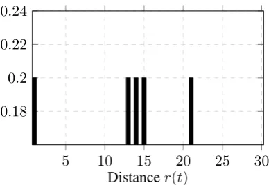
Figures 1 and 2 show distributions of distances r(t) for the simple term ‘algebra’ and the com-plex term ‘nlp’, calculated over the reference col-lection containing 1.5M documents of the Rus-sian Wikipedia. For the ‘algebra’ term most occurrences are relatively close to each other, whether ‘nlp’ occurrences have fairly greater dis-tance scores.
5 10 15 20 25 30 0
0.02 0.04 0.06 0.08 0.1
Distancer(t)
Figure 1: Distribution of distancesr(t), calculated over the complete Wikipedia dataset for the word ‘algebra’.
So, using the formula for c(ti) as above and choosing weightsw(ti)we get the distance-based complexity model.
3.2 Counter-Based Complexity Model
The second model presented in this paper is based on the assumption that each term has an inde-pendent fixed complexity in the whole language. Thus, in this section we consider not the complex-ity distribution of a single term, but the general complexity distribution over all terms in the lan-guage. Hence, each term t is assigned the only
5 10 15 20 25 30 0.18
0.2 0.22 0.24
Distancer(t)
Figure 2: Distribution of distancesr(t), calculated over the complete Wikipedia dataset for the word ‘nlp’.
complexity scorec(t)and theγ-quantile we count is now a constantCγ.
Hence, the model has the following form:
W(d) =
nd X
i=1
w(ti)
1
count(ti) > Cγ
(6)
where w(ti) corresponds to the term weights in-troduced before.
Assume the term t1 is more complex than the
termt2 if number of occurrences in the reference
collection of the termt1is lesser than the number
of occurrences of the termt2.
Letcount(t)denote number of occurrences of the term t in the reference collection. Thus, the complexity score function can be defined as
c(t) = 1
count(t) (7)
so the assumption above is satisfied.
For each termtwe calculate counterscount(t)
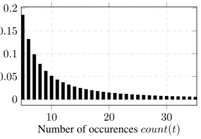
and complexity scoresc(t)over the reference col-lection. Having the distribution ofc(t), we obtain γ-quantilesCγ. The described distribution for the Russian Wikipedia reference collection is shown on Figure 3.
Thus, we have definedc(t)for all terms possible and the distribution necessary to count theCγ. By varying weightsw(ti)described in section 3, we obtain the counter-based model for the complexity estimation.
4 Quality Metric
10 20 30 0
0.05 0.1 0.15 0.2
Number of occurencescount(t)
Figure 3: Distribution of count(t), calculated over complete Wikipedia articles dataset.
more difficult to comprehend. If person cannot de-termine which document is more complex, then he was asked to choose ‘documents are equal’ option. If documents in the given pair are from different scientific domains, then we ask assessor to choose ‘invalid pair’ option.
Documents were chosen from math, physics, chemistry and programming areas. Clustering was performed using the topic modeling technique (Hofmann,1999). BigARTM open-source library was used to perform the clustering (Vorontsov et al.,2015). Pairs were formed so that both doc-uments belong to a single topic and their lengths are almost identical. Examples of document pairs to assess are introduced in Table 2.
Document 1 Document 2 Result
Matrix Tensor RIGHT
Neural network Linear regression LEFT
Electric charge Molecule EQUAL
Mac OS X Convex Hull INVALID
Table 2: Examples of labeled document pairs.
Each pair was labeled twice in order to avoid human factor mistakes. We assume that the pair was labeled correctly if labels were not controver-sial, i.e. first assessor labeled the first document as more complex, while second assessor chose the second document. If one or both grades were ‘doc-uments are equal’ then we assume the pair to be correctly labeled.
8K pairs out of 10K were labeled correctly and were used to compare for the different versions of algorithms. For each we calculated the accuracy score, which is the rate of correctly chosen docu-ment in the pair.
5 Experiments
Two types of experiments were done. In first case we used full Russian Wikipedia articles dataset (1.5M documents) as a reference collection. In second type we used only Wikipedia articles from the math domain. To do that, we built a topic model using ARTM (Additive Regulariza-tion of Topic Models) technique (Vorontsov and Potapenko,2015), which clusters documents into monothematic groups.
5.1 Complete Wikipedia Dataset
Preprocessing: All Wikipedia articles were lem-matized (i.e. reduced to normal form). In this experiment we assume term to be either a single word or a bigram (i.e. two words combination). To extract them, RAKE algorithm (Rose et al.,2010) was used. Hence, each document in the collection was turned into the sequence of such terms.
Reference collection: Preprocessed Wikipedia articles were used as a reference collection. r(t)
for every term position and count(t) for every unique term were counted.
Documents to estimate complexity on: We used the labeled pairs described in Section 4 to evaluate the models. Accuracy was used as a qual-ity metric.
Models to evaluate: Models introduced in 3.1 and 3.2 with differentw(ti) parameters were tested. We took ARI and Flesch-Kincaid readabil-ity test as benchmarks.
The results of the experiments are introduced in Table 3. Also we tested how the bigrams extrac-tion affects final quality with fixed weight funcextrac-tion w(t) =c(t)/nd. The results are given in Table 4.
Model w(t) Accuracy
ARI - 46%
Flesch-Kincaid - 57%
Distance-based c(t) 68%
Distance-based c(t)/nd 71%
Counter-based c(t) 77%
Counter-based c(t)/nd 81%
Table 3: Results of experiment 1 with different weight function.
Results show that both distance- and counter-based approaches work twice as well as readabil-ity indexes. Counter-based model with w(t) =
Model Terms Accuracy
Distance-based Words 63%
Distance-based Words+Bigrams 71%
Counter-based Words+Bigrams 74%
Counter-based Bigrams 81%
Table 4: Results of experiments 1 with terms differ-ently defined.
5.2 Single Topic Wikipedia Dataset
In experiment 2 we shortened the reference collec-tion to include only documents from specific topic.
ARTM model: To divide documents into single-topic clusters, topic modeling is used. Topic Models are unsupervised machine learn-ing models and perform soft clusterlearn-ing (i.e. as-sign each document a distribution over topics). The set of such vectors for all documents form a matrix, which is usually denoted by Θ. ARTM modelwas trained on the preprocessed Wikipedia dataset. ARTM features dozens of various types of regularizers and allows to treat modalities (i.e. types of terms) differently.
In this specific experiment we used regularizers to sparseΘmatrix and make each topic distribu-tion over terms more different. Words and bigrams (i.e. pairs of words) modalities were used with weights 1 and 5 respectively. Using this model, we detect the most likely topic for each document.
Experiment setup: In the following experi-ment we chose math and physics docuexperi-ments to be the reference collection. Documents were prepro-cessed in the same way as they were in the pre-vious experiment. We also divided labeled pairs into same single-topic groups to test models con-figured with different reference collections on var-ious single-topic groups of labeled pairs.
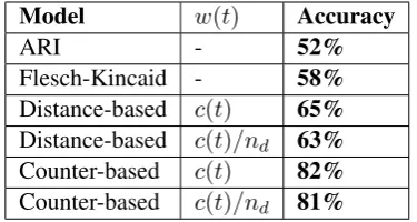
Math collection included 200K documents in reference collection and 3.5K labeled pairs, while for the physics collection it was 250K documents in reference collection and 1.5K labels. The re-sults are shown in Table 5 and Table 6.
As it can be seen from results, using tailored reference collection improves the score. Indeed, that solves terms ambiguity problem and elimi-nates terms unrelated to the topic from the refer-ence collection, so they are treated complex in the estimating document, which is fairly logical.
Model w(t) Accuracy
ARI - 41%
Flesch-Kincaid - 49%
Distance-based c(t) 55%
Distance-based c(t)/nd 61%
Counter-based c(t) 79%
Counter-based c(t)/nd 84%
Table 5: Results of experiment 2 on math collection of Wikipedia articles with different weights.
Model w(t) Accuracy
ARI - 52%
Flesch-Kincaid - 58%
Distance-based c(t) 65%
Distance-based c(t)/nd 63%
Counter-based c(t) 82%
Counter-based c(t)/nd 81%
Table 6: Results of experiment 2 on physics collection of Wikipedia articles with different weights.
6 Conclusions
We have presented an approach to estimating text complexity based on lexical features. Document complexity is an aggregation of terms’ complexi-ties. Introduced general model is highly flexible, it can be adjusted by tuning weightsw(t)and choos-ing proper reference collection.
Complexity score can only be count with re-spect to the reference collection. Reference col-lection can be a large set of documents on different topics or just contain single-topic texts.
The proposed complexity measures are
used in AITHEA exploratory search system (http://aithea.com/exploratory-search) for ranking search results in complexity-based reading order.
Acknowledgements
Application of topic modeling in this research was supported by the Russian Research Foundation grant no. 19-11-00281. The work of K.Vorontsov was partially supported by the Government of the Russian Federation (agreement 05.Y09.21.0018) and the Russian Foundation for Basic Research (grants 17-07-01536).
References
text simplification.
A.A. Birkin. 2007. Speech Codes. Hippocrat, Saint-Peterburg.
Dominique Brunato, Felice Dell’Orletta, Giulia Ven-turi, and Simonetta Montemagni. 2015. Design and annotation of the first italian corpus for text simpli-fication. pages 31–41.
Tim vor der Brck, Sven Hartrumpf, and Hermann Hel-big. 2008. A readability checker with supervised learning using deep syntactic and semantic indica-tors.
Aryna Dzmitryieva. 2017. The art of legal writing: A quantitative analysis of russian constitutional court rulings. Sravnitel’noe konstitucionnoe obozrenie, 3:125–133.
R. Flesh. 1951. How to test readability. New York, Harper and Brothers.
Arthur Graesser, Danielle McNamara, Max Louwerse, and Zhiqiang Cai. 2004. Coh-metrix: Analysis of text on cohesion and language. Behavior research methods, instruments, computers : a journal of the Psychonomic Society, Inc, 36:193–202.
Robert Gunning. 1952.The technique of clear writing. McGraw-Hill, New York.
Thomas Hofmann. 1999. Probabilistic latent semantic indexing. InProceedings of the 22Nd Annual Inter-national ACM SIGIR Conference on Research and Development in Information Retrieval, SIGIR ’99, pages 50–57, New York, NY, USA. ACM.
Georgia Koutrika, Lei Liu, and Steven Simske. 2015. Generating reading orders over document collec-tions. In2015 IEEE 31st International Conference on Data Engineering, pages 507–518.
Gary Marchionini. 2006. Exploratory search: From finding to understanding. Commun. ACM, 49(4):41– 46.
G. H. McLaughlin. 1969. Smog grading: A new read-ability formula. Journal of Reading, 12(8):639–646.
Emilie Palagi, Fabien Gandon, Alain Giboin, and Rapha¨el Troncy. 2017. A survey of definitions and models of exploratory search. InESIDA17 - ACM Workshop on Exploratory Search and Interactive Data Analytics, Mar 2017, Limassol, Cyprus, pages 3–8.
Stuart Rose, Dave Engel, Nick Cramer, and Wendy Cowley. 2010. Automatic Keyword Extraction from Individual Documents.
R.J. Senter and E.A. Smith. 1967. Automated readabil-ity index. AMRL-TR, 66(22).
K. V. Vorontsov and A. A. Potapenko. 2015. Additive regularization of topic models. Machine Learning, Special Issue on Data Analysis and Intelligent Opti-mization with Applications, 101(1):303–323.
Konstantin Vorontsov, Oleksandr Frei, Murat Apishev, Petr Romov, and Marina Suvorova. 2015. Bi-gartm: Open source library for regularized mul-timodal topic modeling of large collections. In
AIST’2015, Analysis of Images, Social networks and Texts, pages 370–384. Springer International Pub-lishing Switzerland, Communications in Computer and Information Science (CCIS).