Measurement of the Neutron Beta Decay Asymmetry using Ultracold Neutrons

(1)

using ultracold neutrons

Thesis by

Michael Praetorius Mendenhall

In Partial Fulfillment of the Requirements for the Degree of

Doctor of Philosophy

California Institute of Technology Pasadena, California

2014

(2)

Michael Praetorius Mendenhall, 2014

this work is released into the public domain by the author, with all copyrights waived to the extent allowed by law

as per CC0 1.0 Universal Public Domain Dedication

(3)

(4)

Acknowledgements

The research presented in this dissertation is the product of a wide-ranging collaboration. I am grateful for many people; not only for their contributions to scientific knowledge, but also for my personal benefit from the privilege of working alongside them. The mentorship and guidance of these colleagues has been the best material from which my graduate education could be made.

I would especially like to acknowledge the Kellogg Radiation Laboratory research group at Cal-tech, including my advisor Brad Filippone, (former) postdocs Jianglai Liu and Brad Plaster; Bob Carr, Pat Huber, and fellow graduate students Kevin Hickerson and Riccardo Schmid. Also, the graduate students from collaborating institutions, with whom I shared many long night shifts on the experiment: Robbie Pattie, Adam Holley, Leah Broussard, Raymond Rios, Brittney VornDick, and Bryan Zeck. The Los Alamos researchers and sta↵: Andy Saunders, Mark Makela, Takeyasu Ito, Chris Morris, Susan Seestrom, Scott Currie; and Albert Young at NCSU.

Thanks also to my parents, Marcus and Cheryl Mendenhall, who preceded me through the experience of graduate studies at Caltech; and to my church family in Pasadena at Trinity Lutheran.

(5)

Abstract

The free neutron beta decay correlation A0 between neutron polarization and electron emission

direction provides the strongest constraint on the ratio = gA/gV of the Axial-vector to Vector coupling constants in Weak decay. In conjunction with the CKM Matrix elementVudand the neutron

lifetime⌧n, provides a test of Standard Model assumptions for the Weak interaction. Leading high-precision measurements ofA0and⌧n in the 1995–2005 time period showed discrepancies with prior measurements and Standard Model predictions for the relationship between , ⌧n, andVud. The

UCNA experiment was developed to measureA0from decay of polarized ultracold neutrons (UCN),

(6)

List of Figures

1 Logo of the UCNA Collaboration. . . iv

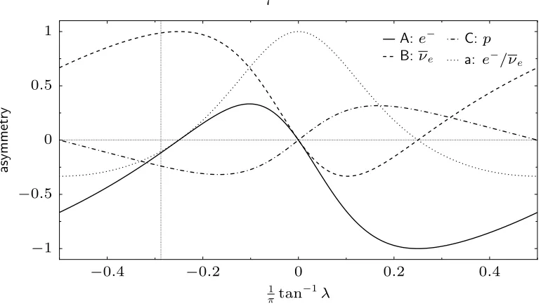
1.1 Dependence of neutron decay correlations on ⌘gA/gV. . . 7

1.2 History ofAexperimental results through 2010. . . 13

1.3 State of Weak interactions experimental field in 2010,Vud- phase space. . . 19

2.1 UCNA experimental hall layout. . . 22

2.2 Sketch of UCN source. . . 23

2.3 Sketch of SCS magnet and detectors. . . 26

2.4 Sketch of SCS detector package. . . 27

2.5 PMT signal chain. . . 31

2.6 UCNA DAQ schematic. . . 32

3.1 Backscattering event topologies. . . 40

3.2 Optimization of wirechamber energy cut for Type II/III event separation. . . 45

3.3 Optimum Type II/III separation wirechamber energy cut. . . 45

3.4 Predicted Type II/III separation accuracy. . . 46

3.5 Evis!Etrue curves. . . 47

3.6 Detector hit positions with three sealed sources in holder. . . 48

3.7 A menagerie of Xenon isotopes, as seen by the UCNA spectrometer (simulated). . . . 51

4.1 MC detector geometry. . . 55

4.2 MC source holder geometry. . . 57

4.3 MC energy deposition in wrinkled foils. . . 60

4.4 Energy loss of241_{Am 5485}_._{56 keV}_↵_{decays through aluminized Mylar foils. . . .} ₆₁

4.5 Sketch of an electron’s trajectory in an expanding magnetic field. . . 62

4.6 Spectrometer magnetic field maps using Hall probe array. . . 64

4.7 Spectrum and corrections for135_Xe 3 2 + beta decay. . . 68

4.8 Corrections to the shape of the neutron beta decay spectrum. . . 69

4.9 MC of scintillator quenching e↵ects for207_{Bi calibration source. . . .} ₇₂

4.10 Geant4 MC backscatter rates versus data. . . 76

5.1 Typical PMT pedestal distributions. . . 78

5.2 PMT pedestal values history. . . 79

5.3 Single-PMT trigger efficiency determination. . . 82

(14)

5.5 207_{Bi pulser spectrum. . . .} ₈₄

5.6 207_{Bi pulser gain monitor history.} _{. . . .} ₈₆

5.7 Sensitivity of Kurie fit to energy resolution, versus fit range upper end. . . 88

5.8 Sensitivity of Kurie fit to energy resolution, versus fit range lower end. . . 88

5.9 Decomposition of observed Xe spectra into isotope components. . . 90

5.10 Xenon spectrum composition change over time. . . 91

5.11 Scintillator light transport maps. . . 93

5.12 Example calibration source peak fits. . . 97

5.13 Example PMT linearity curve from calibration source scan. . . 98

5.14 Energy reconstruction errors for all 2010 calibrations. . . 99

5.15 Example observed versus expected calibration peak widths. . . 100

5.16 Errors in source peak width predictions. . . 102

5.17 Multi-sweep determination of LED averaged output applied to one sweep. . . 105

5.18 Observed scatter in LED sweep data. . . 106

5.19 Estimated LED output fluctuation contribution to total observedE8fluctuations. . . 107

6.1 Examples of wirechamber pedestals. . . 110

6.2 Cathode pedestal histories. . . 111

6.3 Cathode charge cloud size versus anode signal. . . 112

6.4 Anode ADC spectra. . . 113

6.5 Anode ADC spectra most probable values, by position and scintillator energy. . . 114

6.6 Wirechamber energy deposition most probable value by scintillator energy. . . 114

6.7 Position dependence of wirechamber charge signal magnitude. . . 115

6.8 Wirechamber energy deposition, data versus MC. . . 115

6.9 Anode gain calibration factor history. . . 116

6.10 Characteristics of cathode segment readout. . . 119

6.11 Cathode segment event counts prior to gain adjustment. . . 122

6.12 Normalized cathode signal distribution, and sketch of e↵ect of cathode gain changes. . 123

6.13 Cathode segment gain adjustments. . . 124

6.14 Cathode segment event counts after gain correction. . . 124

6.15 Wirechamber positioning correction coefficients. . . 126

6.16 Wirechamber beta decay event positions, before and after uniformity correction. . . . 127

6.17 Wirechamber beta decay event 2D distribution, before and after uniformity correction. 128 6.18 Example position reconstructions of localized event distributions from sealed sources. 128 6.19 Data and simulated cathode charge distributions. . . 129

6.20 East-West event position o↵sets. . . 130

6.21 East-West event position o↵sets history. . . 130

7.1 Simulated detector efficiency⌘s(E). . . 134

7.2 Neutron beta decay statistical sensitivity for extracting asymmetryA0. . . 137

7.3 Accumulated neutron decay statistics for 2010 dataset. . . 138

7.4 MC Backscattering corrections for 2010 geometry. . . 142

7.5 MC acceptance correction 3 and combined 2+ 3for 2010 geometry. . . 144

(15)

7.7 Energy calibration related uncertainties onAin 2010 data analysis. . . 147

7.8 Gamma ray events spectra. . . 152

7.9 Timing coincidence spectra from muon veto detectors. . . 153

7.10 Muon veto scintillator event spectra. . . 153

7.11 Muon-tagged events energy spectra. . . 154

7.12 Muon-tagged event rate in 2010 beta decay runs. . . 154

7.13 Subtracted background energy spectra by identified event type. . . 156

7.14 Background runs event positions. . . 157

7.15 Subtracted background event rate within beta decay analysis cuts. . . 158

7.16 Muon veto efficiency fluctuation uncertainty for 2010 data. . . 158

7.17 Neutron generated backgrounds simulation. . . 160

7.18 Data/MC comparison for high energy excess beta events after background subtraction. 162 7.19 MC estimated neutron generated background. . . 163

7.20 Recoil order and radiative theory modifications to observed asymmetry. . . 163

7.21 Event radial position distributions. . . 167

7.22 Asymmetries for subsets of 2010 data. . . 168

7.23 Beta decay energy spectrum from 2010 dataset. . . 169

7.24 Combined asymmetry from 2010 dataset. . . 169

8.1 Weak decay parameter discrepancies, before and after the UCNA results publication. 172 8.2 History ofAexperimental results. . . 172

A.1 139_{Ce decay source. . . 177}

A.2 113_{Sn decay source.} _{. . . 178}

A.3 207Bi decay source. . . 178

A.4 114m_{In decay source. . . 180}

A.5 109_{Cd decay source. . . 181}

A.6 137_{Cs decay source.} _{. . . 181}

A.7 Simulated detected event positions from gamma rays in sealed source holder. . . 183

A.8 Simulated Compton electron spectra from gamma rays originating in a sealed source. 183 C.1 Square root and inverse square root components for special case matrix. . . 187

(16)

List of Tables

1.1 Neutron potentials from material, magnetic, and gravitational interactions. . . 17

2.1 Beta decay data collection sequences. . . 34

3.1 System response model, connecting initial physics to collected data. . . 38

3.2 Observed backscatter classification. . . 44

3.3 Electron source radioisotopes useful for UCNA calibration. . . 49

3.4 Binding energies for selected conversion electron sources. . . 49

3.5 Xenon isotopes accessible by neutron capture on stable xenon. . . 50

4.1 MC detector geometry materials in electron path. . . 57

4.2 Geant4 simulated energy losses in spectrometer material volumes. . . 59

4.3 Backscatter fractions,Geant4 MC versus data. . . 76

5.1 Pedestal correlations between PMT pairs. . . 107

7.1 UCNA 2010 asymmetry corrections and uncertainties. . . 133

7.2 Neutron polarizations for the 2010 dataset. . . 139

7.3 Neutron-generated background counts, data and simulation. . . 161

(17)

Chapter 1

Historical context for neutron beta

decay measurements

1.1

Development of Weak interactions theory

1.1.1

Beta decay

1.1.1.1 Fermi’s decay theory

Enrico Fermi’s 1934 “Versuch einer Theorie der -Strahlen” (“Attempt at a theory of -rays”) [Fer34] (available in translation [Wil68]) provides a remarkable starting point for the study of beta decays. Fermi describes the interaction through the Hamiltonian

H=Hh.p.+Hl.p.+Hint, (1.1)

constructed from the heavy particle (nucleon) energies Hh.p., light particle (lepton) energies Hl.p.,

and an interaction termHint, which permits transition between the initial and final states in

pertur-bation theory. Following a series of simplifying assumptions for the form of the interaction, Fermi concludes a plausible form for changing between a neutron and proton while producing an electron and antineutrino,

Hint=g[Q( 1 2+ 2 1+ 3 4 4 3) +Q⇤( ⇤1 ⇤2+ 2⇤ ⇤1+ 3⇤ ⇤4 4⇤ ⇤3)], (1.2)

whereg is the coupling strength constant,QandQ⇤ are operators changing a proton to a neutron and vice-versa, i are the four components of the relativistic Dirac wavefunction for annihilation ( ⇤

i for creation) of the electron, and i for the (anti)neutrino. The particular combination of ’s and ’s chosen came from analogy to the electromagnetic interaction HEM=eJµAµ, treating the lepton term as transforming like electromagnetic vector four-potential component A0 (and taking

the nucleus’ contributionJµ in the nonrelativistic limit). In more modern notation, Fermi’s Vector interaction would be written:

(18)

From this reasoning, and incorporating Coulomb interactions for the outgoing electron based on hydrogen atom wavefunctions, Fermi proposed the electron energy spectrum form resulting in

SFermi(W)dW ⌘G2|M|2F(Z, W)(W0 W)2

p

W2 ₁_{W dW,} _(1.4)

where W is the electron total energy in mec2 units, W0 is the decay endpoint energy, |M|2 is

the matrix element between initial and final nuclear states, Gan overall coupling constant for the interaction, and F(Z, W) is the Fermi function incorporating Coulomb interaction e↵ects on the electron’s decay phase space:

F(Z, W)_⌘ 4

(3 + 2 )(2p⇢)

2 _e⇡↵ZW/p

| (1 + +i↵ZW/p)_|2, _⌘p1 (↵Z)2 ₁_{, p}₌p_W2 ₁_,

(1.5) where⇢is the radius of the nucleus.

1.1.1.2 Konopinski-Uhlenbeck modification

Comparing Fermi’s decay spectrum form with available experimental data, Konopinksi and Uhlen-beck published a 1935 article [KU35] noting a systematic tendency for measured spectra to show a more asymmetric form (biased towards lower energies) than Fermi’s proposed form. They proposed a modification to the “statistical factor” for the decay phase space S (produced by assuming coupling to the neutrino wavefunction’s gradient rather than its value), changing Fermi’s prediction for the decay spectrum to a re-weighted form:

SFermi(W)dW !SK-U(W)dW ⌘G2|M|2F(Z, W)(W0 W)4

p

W2 ₁_{W dW.} _(1.6)

The Konopinski-Uhlenbeck spectrum shape, with its additional factor of (W0 W)2,

gener-ally produced better agreement with experimental beta spectra shapes at the time, and gained widespread popularity in the beta decay physics community. However, as experimental technique improved over the next several years, beta decay spectra “shifted” from agreeing better with the K-U form back towards Fermi’s original theory.

In a 1943 review article on beta decay, Konopinski writes:

“Thus, the evidence of the spectra, which has previously comprised the sole support for the K-U theory, now definitely fails to support it.” [Kon43]

Among the main culprits identified by Konopinski for the discrepancies between earlier and later experimental results were extra energy losses in older thick decay source samples, distorting the spectrum towards the K-U form; development of newer, thin decay samples agreed better with Fermi’s predictions.

1.1.1.3 What interaction form?

(19)

evidence from thorium beta decays, which instead favored the Gamow-Teller (G-T) selection rules of J = 0,_±1 (except 0_!0), no parity change. Either a Tensor or Axial-Vector decay form would produce the G-T selection rule, while both Vector and Scalar forms produce the Fermi selection rule. A Pseudoscalar interaction would produce J= 0 with parity change.

As Konopinski discusses in [Kon43], each individual interaction form would produce the same allowed beta decay spectrum shape. However, a 1937 paper by Markus Fierz [Fie37] noted that the simultaneous presence of both Tensor and Axial-vector terms, or of both Scalar and Vector terms, would produce interference cross-terms modifying the spectrum shape. Which interaction forms actually dominated in beta decay would remain an open question for the next 15 years, with confusing and contradictory experimental evidence.

1.1.2

The Weak interaction

1.1.2.1 Universal Weak interaction

In 1949, Tiomno and Wheeler commented on a striking similarity between the interactions n _! p+e+⌫e,µ !e+⌫e+⌫µ, andµ +p!n+⌫µ:

“We note that the three coupling constants determined quite independently agree with one another within the limits of error of experiment and theory. We apparently have to do in all three reaction processes with phenomena having a much closer relationship than we can now visualize.” [TW49]

A contemporaneous letter by Lee, Rosenbluth, and Yang commented on the same coincidence:

“One can perhaps attempt to explain the equality of these interactions in a manner analogous to that used for the Coulomb interactions, i.e. by assuming these interactions to be transmitted through an intermediate field with respect to which all particles have the same “charge.” The “quanta” of such a field would have a very short lifetime and would have escaped detection.” [LRY49]

Progress in experimental measurements of such interactions solidified the hypothesis of a common mechanism, named the “Weak” interaction in comparison to the higher energy scales and faster decays of the Strong nuclear interaction. Fermi’s theoretical framework for beta decay now came to encompass a wide variety of four-Fermion Weak interactions.

1.1.2.2 Parity-violating interaction terms

In an October 1956 paper [LY56], Lee and Yang proposed expanding the terms in the Weak inter-action neutron decay Hamiltonian:

Hint= ( p n)(CS e ⌫e+CS0 e 5 ⌫e)

+ ( p µ n)(CV e µ ⌫e+C

0

V e µ 5 ⌫e)

+1

2( p µ n)(CT e µ ⌫e+C

0

T e µ 5 ⌫e)

( p µ 5 n)(CA e µ 5 ⌫e+CA0 e µ ⌫e)

( p 5 n)(CP e 5 ⌫e+CP0 e ⌫e) + H.C.,

(20)

in which theCicoupling constants prefix the Scalar, Vector, Tensor, Axial-vector, and Pseudo-scalar terms of prior Fermi theory. TheCi0 couplings, however, introduce new parity-violating terms. In the caseC0

i =±Ci, the (1± 5) terms indicate maximal parity violation in which only one helicity

of the leptons participates — right-handed neutrinos for (1 + 5) and left-handed for (1 5), with

the electron helicity identical in theV andAcases, or opposite inS,T,P.

Parity violation had been excluded in Strong interactions with stringent experimental limits, and thus it had not been previously considered in Weak decay theory. However, Lee and Yang noted that there had been no conclusive experimental tests of parity conservation in Weak decays. Furthermore, parity violation could solve an open puzzle about experimentally observed “⌧+_{” and}

“✓+_{” particles, which appeared to have the same masses and lifetimes, but decayed to states with}

opposite parity. “One way out of the difficulty,” wrote Lee and Yang, “is to assume that parity is not strictly conserved, so that ✓+ _and _⌧+ _{are two di}_↵_{erent decay modes of the same particle,}

which necessarily has a single mass value and a single lifetime.” Lee and Yang proposed a variety of experimental observables that would result from parity violation, including:

“A relatively simple possibility is to measure the angular distribution of the electrons coming from decays of oriented nuclei. If✓is the angle between the orientation of the parent nucleus and the momentum of the electron, an asymmetry of distribution between

✓and 180 ✓constitutes an unequivocal proof that parity is not conserved in decay.”

Prompted by Lee and Yang, Chien-Shiung Wu quickly assembled an experiment to test the theory. In January 1957, Wu published a measurement of the parity-violating electron asymmetry in polarized

60_{Co beta decay [Wu+57]. Experimental evidence indicated not only that parity violation occurred}

in Weak decays, but also that parity violation was maximal within experimental uncertainties. Lee and Yang shared the 1957 Nobel Prize in Physics, and the “✓+_{” and “}_⌧+_{” mesons are known today}

as the Kaon K+_{. The apparent completeness of parity violation led Lee and Yang to propose a}

two-component neutrino theory in which only one neutrino handedness was produced in beta decay [LY57] (though it was not known which one).

1.1.2.3 Decay correlations

Decay angular correlations (and improved experimental capabilities to measure them) opened up a new window for understanding Weak interactions beyond spectrum shapes and decay lifetimes. Jackson, Trieman, and Wyld considered a variety of other experimentally observable correlations in a pair of papers early in 1957 [JTW57b; JTW57a] (with additional correlation termsI,K0_,_M_,_S_,_T_,

U,V,W enumerated in a follow-up article by Ebel and Feldman [EF57]). The ⌥-decay rate for an ensemble of nuclei with chargeZ_⌥1, angular momentumJ in direction ˆ|, as a function of electron momentum and energy pe and Ee, neutrino momentum and energy p⌫ and E⌫ (experimentally

(21)

(22)

Weak decays involved Vector and Axial-vector couplings, with coupling constants approximately equal in magnitude and opposite in sign, called the “V Astructure” of the Weak interaction.

1.1.2.5 Conserved Vector Current hypothesis

A 1955 article by USSR theorists Gershtein and Zeldovich [GZ56] had noted a special property of Vector interaction contributions to Weak decay. However, due to the presumed Scalar/Tensor form at the time, Gershtein and Zeldovich’s observation received little immediate attention:

“It is of no practical significance but only of theoretical interest that in the case of the vector interaction typeV we should expect the equality

gF(V)⌘gF0(V)

to any order of the meson-nucleon coupling constant, taking nucleon recoil into account and allowing also for the interaction of the nucleon with the electromagnetic field, etc. This result might be seen by analogy with Ward’s identity for the interaction of a charged particle with the electromagnetic field; in this case virtual processes involving particles (self-energy and vertex parts) do not lead to charge renormalization of the particle.”

Renewed interest in Vector interactions, along with experimental evidence, prompted Feynman and Gell-Mann to independently rediscover Gershtein and Zeldovich’s observation. Feynman and Gell-Mann begin a 1958 article [FGM58] noting the agreement between the muon lifetime calculated using the coupling constantGderived from O14 + _decay,_⌧

µ= 192⇡3/G2µ5= (2.26±0.04)⇥10 6 seconds, and the direct experimental measurement of⌧µ = (2.22±0.02)⇥10 6 seconds:

“It might be asked why this agreement should be so good. Because nucleons can emit virtual pions there might be expected to be a renormalization of the e↵ective coupling constant. On the other hand, if there is some truth in the idea of an interaction with a universal constant strength it may be that the other interactions are so arranged so as not to destroy this constant. We have an example in electrodynamics.”

Feynman and Gell-Mann proposed that, analogous to conserved electric charge, the Weak decay vector coupling was associated with a current that “is conserved, and, like electricity, leads to a quantity whose value (for low energy interactions) is unchanged by the interaction of pions and nucleons.” This principle came to be named the “Conserved Vector Current” (CVC) hypothesis.

(23)

(24)

neutrally charged, pointlike proton. To distinguish this “bare model parameter” value from the physical asymmetry that will be observed in the lab, theAof Equation 1.12 is often denoted “A0.”

1.1.2.7 Induced couplings

Goldberger and Treiman published a Physical Review article in 1958 [GT58] noting that, while the Weak decay Lagrangian contained onlyV Aterms for the lepton couplings, additional terms with di↵erent symmetries could be induced in decay matrix elements by Strong interaction e↵ects. While these induced couplings would likely be “negligible in decay,” the higher momentum transfer inµ

capture interactions might demonstrate induced pseudoscalar terms.

1.1.2.8 Weak Magnetism

In the same edition of Physical Review containing Goldberger and Treiman’s article on induced couplings, Gell-Mann followed the Weak interaction’s analogous mathematical structure to electro-magnetism to note that the Vector interaction also

“...gives rise to ‘weak magnetism’ analogous to the magnetic e↵ects that induce the emission of M1 photons. This ‘weak magnetism’ obeys Gamow-Teller selection rules and interferes with theAcoupling...” [GM58]

Gell-Mann proceeds to calculate the e↵ect on thee -⌫ angular correlation and the electron energy spectrum.

Bilen’ki˘ıet al. [Bil+60] expanded the calculation to other neutron -decay observables. They found that the neutron -decay correlation coefficientAwould pick up an energy dependence from the recoil-order terms:

ARO(E) =A 0+

2( +µ) (1 + 3 2₎2

1

M

✓

2₊2

3 1 3

◆

E0

✓

3_{+ 3} 2₊5

3 1 3

◆

E 2 2₍ ₁₎m2e

E ,

(1.14)

whereµ⌘µp µn, withµp⇡2.79 andµn⇡ 1.91 as the proton and neutron magnetic moments,

E as the decay electron’s total energy, and _⌘_|gA/gV|. The net e↵ect is an⇠1.5% increase of the physical asymmetry overA0, shown in Figure 7.20.

1.1.2.9 Second-class currents

Unlike the Strong interaction, the Weak interaction had been demonstrated to violate Parity try. Weinberg considers in [Wei58] the implications of applying another Strong interaction symme-try,G_⌘Cei⇡I2 _{(the product of charge symmetry and charge conjugation), to the Weak interaction.}

(25)

(26)

which modifies the observable asymmetry by the factor ↵

2⇡(h g)⇠10

3_,

h g= 4

✓_tanh 1

1 ◆ ✓

1 2+E0 E

8E

◆_E

0 E

3E 2 +

tanh 1 ✓

2 2 2 (E0 E)

2

6E2

◆

,

(1.18) whereE0 is the neutron -decay endpoint, andE, ⌘v_c are the electron’s total energy and speed.

The result is an⇠0.1% increase of the physical asymmetry overA0, shown in Figure 7.20.

1.1.3

Connection to quark model

1.1.3.1 Quarks

By mid-century, particle physics experiment had uncovered a large and still growing catalog of new particles. Shoichi Sakata commented in a 1956 letter:

“It seems to me that the present state of the theory of new particles is very similar to that of the atomic nuclei 25 years ago. At that time, we had known a beautiful relation between the spin and the mass number of the atomic nuclei. Namely, the spin of the nucleus is always integer if the mass number is even, whereas the former is always half integer if the latter is odd. But unfortunately we could not understand the profound meaning for this even-odd rule.” [Sak56]

As the discovery of the neutron led to an explanation for nuclear properties in terms of proton and neutron constituents, Sakata was hopeful that properties of the zoo of newly discovered particles could likewise be explained:

“In our model, the new particles are considered to be composed of four kinds of funda-mental particles in the true sense, that is, nucleon, antinucleon,⇤0 _{and anti-}_⇤0_.”

Murray Gell-Mann and Yuval Ne’eman (independently) developed a more advanced replacement for Sakata’s four-constituent model, associating the organization of baryons and mesons with the mathematical structure of direct products ofSU(3) groups, which Gell-Mann named the “eightfold way”. Gell-Mann distanced the “eightfold way” theory from Sakata’s concept of physical fundamen-tal constituent particles “in the true sense,” emphasizing that the group-theoretical approach was a mathematical abstraction rather than a combination of physical constituents:

“Unitarity symmetry may be applied to the baryons in a more appealing way if we abandon the connection with the symmetrical Sakata model and treat unitarity symmetry in the abstract. (An abstract approach is, of course, required if there are no “elementary” baryons and mesons.)” [GM62]

(27)

“It is fun to speculate about the way quarks would behave if they were physical particles of finite mass (instead of purely mathematical entities as they would be in the limit of infinite mass). Since charge and baryon number are exactly conserved, one of the quarks (presumably u23 or d 13) would be absolutely stable, while the other member of the

doublet would go into the first member very slowly by -decay or K-capture.” [GM64]

1.1.3.2 Cabibbo mixing angle and the charm quark

Experimental measurements of Weak interactions of new particles placed a strain on the CVC hypothesis, indicating higher Vector coupling for particles with strangeness inconsistent with the “universality” of the interaction. In 1963, Nicola Cabibbo extended the CVC hypothesis [Cab63] to account for strangeness-nonconserving decays by describing the Weak interaction Vector current as a mixing of ✓c ⇡ 0.26 between S = 0 and S = 1 currents such that the strength of the combined vector currentj=j S=0cos✓c+j S=1sin✓c would still be “universal.” For Weak decays of particles without strangeness, the Vector decay rate would be scaled down by a factor of cos2_✓

c. Bjørken and Glashow proposed adding a fourth, heavier “charm” quark, incorporating Cabibbo’s mixing angle into the model, explaining the masses of observed mesons, and predicting new decays:

“The model is vulnerable to rapid destruction by the experimentalists. The main pre-diction is the existence of the charmedS+

p,v andDp,v+,0mesons which can be produced in pairs in ⇡ p, K pandp preactions, followed by weak but rapid decays into both Y-conserving and Y-violating channels.” [BG64]

Following experiments contradicted Bjørken and Glashow’s decay predictions, providing “rapid de-struction” for the model. A 1970 paper revived the possibility of the charm quark with the “Glashow-Iliopoulos-Maiani” (GIM) mechanism [GIM70], which re-introduced the fourth quark to explain ex-perimentally observed suppression of S= 2 decays, while also justifying the prior lack of evidence for charm decays:

“such events will necessarily be of very complex topology, involving the plentiful decay products of both charmed states. Charmed particles could easily have escaped notice.”

Independent experiments at BNL [Aub+74] and SLAC [Aug+74] simultaneously announced the discovery of a new particle decay in November 1974, which turned out to be the same cc “J/ ” meson. Burton Richter and Samuel Ting, the lead investigators for each experiment, shared the 1976 Nobel Prize in Physics for the discovery.

1.1.3.3 CKM matrix and unitarity

Meanwhile, a 1973 paper by Kobayashi and Maskawa [KM73] argued that CP-violating Weak decays could only be incorporated into the existing theoretical framework by extending Cabibbo’s two-element mixing angle ✓c to a 3⇥3 unitary mixing matrix — later named the Cabibbo-Kobayashi-Maskawa (CKM) matrix with elements Vij — consequently predicting the existence of yet another generation of quarks. CP violation had been observed in rareK0

2 !⇡⇡ decays in 1964 [Chr+64],

(28)

“bottom” quark in the new pair, while observation of the heavier “top” quark by the D0 [Aba+95] and CDF [Abe+95] experiments was published in 1995. Kobayashi and Maskawa shared in the 2008 Nobel Prize for predicting the third quark generation.

With three generations of quarks discovered, an obvious question is whether there are yet more to be found (extending the CKM matrix to a 4⇥4 mixing). If interactions with a fourth generation are possible, then the existing 3_⇥3 CKM matrix would not be unitary. The first row of the CKM matrix, involving the most common decays coupling to the u quark, provides the most stringent experimental limits on unitarity,i.e. whether_|Vud|2+|Vus|2+|Vub|2= 1.

1.1.4

Beta decay in the Standard Model

Lee and Yang’s e↵ective Hamiltonian model for Weak decays can now be understood in terms of Standard Model quark interactions. Following a 2010 review paper by Towner and Hardy [TH10], the total decay rate for nuclear beta decays will be:

=⌧ 1₌G2FgV2m5e 2⇡3 V

2

udf[|MF|2+ 2|MGT|2], (1.19)

wheref is a phase space integral over the decay spectrum shape,

f _⌘

Z W0

1

(W0 W)2pW F(W, Z)S(W, Z)dW; p⌘

p

W2 ₁_, _(1.20)

where W is the total electron energy (in electron mass units) out to the spectrum endpoint W0,

F(W, Z) is the Fermi function Coulomb correction, and S(W, Z)_⇡1 is all other fine shape correc-tions.

The Fermi coupling constant GF/(~c)3 = 1.1663787(6)·10 5GeV 2 [Ber12] is experimentally

determined from the muon decay lifetime (µ _!⌫µ+⌫e+e ), taking advantage of the universality of the Weak interaction to extract this parameter from a decay independent of nuclear structure considerations. The best experimental measurements of Vud come from from superallowed 0+ !

0+ _{nuclear decay rates, which selection rules guarantee to be pure Fermi decays (}

|MGT|2 = 0).

Combining several experimental results gives the best estimate [HT09]Vud= 0.97425(22).

Free neutron beta decay provides an ideal system for precision measurements of parameters related to Axial-vector contributions to decay, as the nuclear matrix elements are known by definition (|MF|2⌘1,|MGT|2⌘3), rather than requiring difficult and uncertain nuclear structure calculations.

For free neutron beta decay, this yields the relation betweenVud, neutron lifetime ⌧n, and ⌘ _ggA_V [TH10]:

Vud2 =

(4908.7±1.9) s

⌧n(1 + 3 2)

, (1.21)

with neutron decay experiments providing both the lifetime⌧nand the Axial-vector/Vector coupling ratio via the polarized decay correlationA.

1.2

-decay asymmetry experiments

Figure 1.2 shows the history ofA0measurements through 2010, described in the following sections.

(29)

0.1225

0.12

0.1175

0.115

0.1125

0.11

0.1075

0.105

A0

1970 1980 1990 2000 2010

Year CN experiments

UCNA

Figure 1.2: History of A experimental results through 2010 (see Figure 8.2 for inclusion of latest results). In time order as shown: [KR75; Bop+86; Ero+90; Sch+95; Yer+97; Abe+97; Abe+02; Pat+09; LMH+10].

neutrons (CN) from nuclear reactors.

1.2.1

Early

A

measurements at Argonne

The first experimental measurement ofAwas carried out at Argonne National Laboratory and pub-lished by Burgy et al. in September 1957 [Bur+57]. A collimated beam of reactor neutrons was polarized to 87_±7% by glancing reflection from a magnetized cobalt-iron mirror. The neutrons’ polarization could be reversed by reversing the magnetizing field applied to the mirror, and subse-quently depolarized by insertion of an 0.010 inch thick steel plate in the beam path. The neutron beam passed through a decay region with a scintillator beta detector on one side, and a 12 kV accel-erating potential to collect protons on a proton-sensitive cathode (a red-hot beryllium copper ellipse replacing the photocathode at the start of a PMT electron-multiplying dynode stack). Electron-proton coincidence rates (of_⇠9 counts per hour) with the neutron polarization directed towards or away from the beta scintillator, or depolarized by the steel plate, indicated a decay asymmetry of

A= 0.37(11).

Incremental improvements to the Argonne apparatus produced a series of increasingly preciseA

results. From measuring the recoiling proton, the apparatus could also be reconfigured for sensitivity to the correlations BhJi·p⌫

JE⌫ and D

hJi·(pe⇥p⌫)

JEeE⌫ . With an improved proton detector, moved closer

to the neutron beam for increased collection efficiency, the Argonne group produced a result of

(30)

1.2.2

High rate experiments with Perkeo at ILL

A new experimental design, thePerkeospectrometer, was built at the Institut Laue-Langevin (ILL) research reactor in Grenoble, and published its first measurement in 1986 [Bop+86]. A beam of cold neutrons (thermalized in a 23 K deuterium moderator volume near the reactor core) was polarized to

>97% by reflection from a supermirror polarizer. A “current-sheet non-adiabatic spin flipper” could flip the neutron polarization on demand. The polarized neutron beam was directed along the central axis of a 1.7 m long solenoid magnet. At both ends of the solenoid, the magnetic field bent out of the neutron beam path, towards a pair of electron-detecting plastic scintillators. Electrons from neutron decay in the solenoid were confined by the magnetic field and directed towards the detectors on either side. This allowed for a much larger neutron decay region than the Argonne apparatus, with 2_⇥2⇡ angular coverage for electron detection. An unprecedented beta decay detection rate of⇠100 Hz allowed a precision measurement ofA0= 0.1146(19). However, the “bent” magnetic

field configuration produced an _⇠ 10% correction to A0 for magnetic mirroring of electrons from

decays in the field bend regions.

1.2.3

PNPI and ILL TPC measurements

Meanwhile, at the research reactor of the Leningrad Institute of Nuclear Physics (later renamed the Petersburg Nuclear Physics Institute, PNPI), a new liquid hydrogen cold neutron source with an iron-cobalt polarizing mirror was built in 1985. A neutron decay asymmetry experiment at the cold neutron source collected data in 1989–1990, and published results in 1990–1991 [Ero+90; Ero+91]. The detector apparatus was similar to the Argonne experiment, using coincidences between an electron scintillator detector and a proton collector. At a detected event rate of _⇠ 3 Hz, the PNPI experiment had much greater statistical reach than the Argonne measurements, without the large magnetic mirroring systematic corrections of the higher-rate Perkeo spectrometer. With a measured result ofA0= 0.1116(14), however,

“A comparison of the results with the most recent measurements of the neutron life-time and the angular-correlation constant A shows an appreciable deterioration in the consistency of these data.” [Ero+90]

In order to resolve the discrepancy, a di↵erently designed apparatus was built at ILL [Sch+95; Lia+97]. The polarized cold neutron beam passed through a gas-filled drift chamber between two scintillator plates. The gas volume operated as a Time Projection Chamber (TPC), in which the ionization paths left by a decay electron drifted out (at a known rate) to crossed anode and cathode wires, allowing 3-D reconstruction of the electron’s path. The scintillators measured the energy of the electron. The experimental result of A0 = 0.1160(15) was in agreement with Perkeo, but

2.2 from PNPI.

A correction to the 1990 PNPI result was published in 1997 [Yer+97]. Re-analysis of the data accounted for previously ignored distortion of the neutron beam energy spectrum from passage through aluminum windows and air gaps in the beam line. Di↵erences in beam line geometry between the setup for measuring neutron polarization and the setup for beta decay meant that neutron polarization during asymmetry measurement was di↵erent from that directly measured. The re-analyzed result ofA0= 0.1135(14) was in agreement with both thePerkeo[Bop+86] and

(31)

1.2.4

Perkeo II

In 1997, a newly designedPerkeo IIspectrometer at ILL published its first measurement [Abe+97]. Unlike the originalPerkeospectrometer, inPerkeo IIthe magnetic solenoid is placed perpendic-ular to the cold neutron beam. Electron detectors at each end of the solenoid are further from the neutron beam (reducing backgrounds), and because the magnetic field does not need to curve out of the neutron beam path, the large magnetic mirroring corrections are eliminated. The experimental result ofA0= 0.1189(12), however, was in 3 disagreement with the prior world average.

ThePerkeo IIcollaboration worked to double-check their main experimental systematics (po-larization, backgrounds, and detector energy response), publishing a new higher precision measure-ment in 2002 [Abe+02]. The 2002 Perkeo II measurement agreed with their 1997 number — producing a combined result of A0 = 0.1189(7) — still in stark disagreement with the preceding

PDG world average. The paper was provocatively titled “Is the Unitarity of the Quark-Mixing CKM Matrix Violated in Neutron -Decay?”

1.3

Ultracold neutrons

This discrepancy between cold neutron beam measurements of neutron decay parameters encouraged the development of alternative experimental methods that would not share common sources of systematic uncertainty. Ultracold neutrons (UCN) o↵ered such a possibility.

1.3.1

Slow neutron scattering

Enrico Fermi published a long article in the Italian journal La Ricerca Scientifica in 1936 entitled

“Sul moto dei neutroni nelle sostanze idrogenate” (“On the motion of neutrons in hydrogenous substances”) [Fer36]. In this paper, Fermi developed a theory to trace the interaction of neutrons with hydrogen-bearing materials (specifically paraffin), all the way from high-velocity elastic and inelastic scattering to final capture to deuterium. Section (10) of Fermi’s paper,“Urto di neutroni contro atomi di idrogeno legati”(“Scattering of the neutron from bound hydrogen atoms”), focuses on the<1 eV scattering regime where the hydrogen nuclei are held in place by chemical forces in the solid. Fermi develops an approximation based around an intermediate length scaleR, which is simultaneously much greater than the neutron-proton interaction range ⇢and much smaller than the de Broglie wavelength scale for the neutron and proton.

In this regime, the fine details of nucleon interactions may be approximated by a steep-edged potential well, characterized by a single “scattering length”a⌧ . In the limit where the hydrogen nucleus is free to recoil, conservation of momenta indicates acute-angle scattering of the neutron with di↵erential cross section

d!= 4a2_cos_✓_d_!

) tot⌘

Z

d!= 4⇡a2_, _(1.22)

where✓2 ⇡

2,

⇡

2 is the angle between incoming and outgoing neutron momenta in the

(32)

place by chemical bonds in matter, the scattering becomes isotropic with increased cross section

d!= ✓

Mn

µ a

◆2

d!)

Z

d!= 4⇡

✓

Mn

µ a

◆2

, (1.23)

as if the “hard sphere” potential had expanded to the “bound nucleus scattering length”aB⌘ M_µna [GRL91], whereµ_⌘ MnMN

Mn+MN is the reduced mass of the neutron-nucleus system.

When a neutron with wavelength larger than inter-atomic spacings encounters an array of nuclei in matter, coherent scattering over the many individual nuclei produce an e↵ective “Fermi potential” averaged over individual interactions [GRL91],

VF=

2⇡_~2

Mn

naB (1.24)

where n is the number density of the nucleus with bound scattering length aB. For materials with multiple types of nuclei, this may be summed over each variety. Neutrons incident on a material surface with perpendicular kinetic energy lower than the Fermi potential will be entirely reflected. Experiments by Fermi and Zinn in 1946 [FZ46] and Fermi and Marshall in 1947 [FM47], using neutron beams at glancing incidence on various material surfaces, verified Fermi’s low-velocity neutron-scattering theory.

1.3.2

Ultracold neutrons

Zeldovich first published the idea of completely trapping neutrons using the Fermi potential in 1959:

“Let us place neutrons in a cavity surrounded on all sides by graphite. The neutrons of speed higher than critical will rapidly leave the cavity, but neutrons of less than critical speed are blocked in the cavity and vanish only as they decay, with a half-life of approximately 12 minutes.” [Zel59]

The low-kinetic-energy range of neutrons that may be completely trapped by material potentials came to be called “ultracold neutrons” (UCN). Table 1.1 lists the Fermi potential for several mate-rials, along with magnetic and gravitational neutron interactions. Typical Fermi potentials on the order of 200 neV indicate that trapped UCN will have velocities .6 m/s. In addition to reflection from material Fermi potentials, UCN lie in a kinetic energy range where gravitational and magnetic

µ_·B interactions are significant. The magnetic interaction of_±60 neV/T means that several Tesla fields available in the lab can be used to manipulate and sort UCN by spin state. The gravitational potential of 102 neV/m allows acceleration and deceleration of UCN populations by meter-scale drops and rises in containing guides.

Practical realization of Zeldovich’s proposed trapping would be slow in coming, for a variety of reasons. The first difficulty, discussed in the Zeldovich paper, is obtaining in the first place a flux of sufficiently slow neutrons — in a room-temperature thermal distribution, only a tiny portion of neutrons (_⇠ 10 8_{) are in the UCN range that can be completely trapped. Thermalization to}

liquid helium temperatures increases the fraction to _⇠10 5_{. Beyond the initial di}_ffi_{culty of UCN}

(33)

material potential [neV]

58_Ni ₃₃₅

diamond 304

beryllium 252

beryllium oxide 261

stainless steel 188

graphite 180

copper 168

aluminum 54

1T magnetic fieldµn·B ±60

1m risemngh 102

1m/s velocity 1 2mnv

2 _5.2

Table 1.1: Neutron interaction Fermi potentials for various materials [GRL91], along with magnetic and gravitational potentials and kinetic energy.

1.3.3

Early experimental UCN sources

Much of early UCN research took place in the USSR, starting with the first observation of UCN in moderated reactor neutrons [Lus+69; Ign90]. Early experiments used solid-state “converter” sources [Ign90], cooled blocks of moderating material with low Fermi potential (such as aluminum) allowing UCN in the tail of the Maxwell spectrum to escape. Advancements in converter materials and design improved the efficiency of extracting neutrons from the low-temperature tail of the Maxwellian dis-tribution; however, these methods produced experimental UCN fluxes typically measured in counts per hour.

1.3.4

High flux UCN turbine sources

To circumvent the limitations of the Maxwell distribution, Steyerl constructed a “neutron turbine” in 1975 at the FRM reactor in Munich [Ste75], in which a cold neutron beam is incident on the high-Fermi-potential vanes of a quickly rotating turbine. Another UCN turbine was built by Kashoukeev in the same year [Kas+75] at the Institute of Nuclear Research and Nuclear Energy of the Bulgarian Academy of Sciences. The turbine vanes move in the direction of the neutron beam; cold neutrons moving forward slightly faster than the turbine vanes (with UCN velocities relative to the vanes’ reference frame) are reflected to lower velocities in the lab frame, and inward towards slower-moving portions of the vanes nearer the turbine axis. After several reflections, cold neutron portions of the incident Maxwellian distribution — with considerably higher flux than the UCN tail — are converted to UCN. The Steyerl design uses a curved blade geometry with UCN extracted opposite the incoming beam, while the Kashoukeev turbine uses flat blades and extracts UCN from a guide along the turbine axis.

(34)

1.3.5

LANL SD

2

superthermal UCN source

An alternate method for “superthermal” UCN production (boosting the UCN density above the thermal equilibrium distribution) was proposed by Golub and Pendlebury in 1975 [GP75]. Incoming cold neutrons enter a cryogenic crystal, with phonon vibration modes in the right energy-momentum ranges that a neutron scattering o↵ the crystal lattice will dump most of its kinetic energy into exciting a phonon and be left in the UCN velocity range. Because downscattering to UCN can occur for neutrons entering the crystal from a wide range of directions (rather than the collimated cold neutron beam geometry required by turbines), more UCN can be generated from a lower initial cold neutron flux. This permits UCN production from a small pulsed spallation target source, rather than a reactor neutron port.

A prototype solid deuterium (SD2) source was built and tested at the Los Alamos Neutron

Science Center (Lansce) at Los Alamos National Labs (LANL) in 1998–2000 [Liu02]. A few µA from the Lansce800MeV proton accelerator, striking a spallation tungsten target, provided the initial free neutrons, subsequently thermalized in layers of cold polyethylene before downscattering in the SD2 volume (see Figure 2.2 and subsection 2.1.1). Continued development of the LANL

UCN source [Sau+04; Sau+13] turned the prototype source into a facility for experimental neutron research.

1.4

The UCNA experiment

1.4.1

Initial development

Motivated by the discrepant state of cold neutronAmeasurements in 1998, the UCNA experiment was proposed to the DOE in April 2000, to use the LANL SD2UCN source to measureA. Progress

from design to prototype to data-ready experiment is described in [Yua06].

Employing ultracold neutrons for the measurement held the prospect of greatly reducing, or at least providing independent alternatives to, the major systematic concerns associated with cold neutron beam experiments. Backgrounds would be significantly reduced by operating the apparatus away from the higher-radiation environments produced in the path of neutron beams. Neutron polarization would be independent from the systematic uncertainties of beam polarization techniques (though new approaches would be needed for assessing bottled neutron depolarization). The design choice to include a position-tracking wirechamber would trade some additional electron energy losses and backscattering for the advantage of a well-defined fiducial volume and ability to analyze position-dependent detector response. In addition, the wirechambers would provide strong suppression of gamma ray backgrounds.

1.4.2

Neutron lifetime discrepancy

(35)

0+!0+

n PDG

n Sereb

rov

PERKEO

II

’02

PDG

2010

0.97 0.972 0.974 0.976 0.978

Vud

1.265 1.27 1.275 1.28 1.285

| | |gA/gV|

Figure 1.3: State of Weak interactions experimental field in 2010,Vud- phase space. PDG 2010⌧n,

Vud, and [Nak10], versusPerkeo II2002 [Abe+02] and Serebrov 2005⌧n [Ser+05].

(885.7±0.7) s. Serebrov’s lifetime measurement allowed much smaller corrections for non-decay neutron losses than prior experimental work — but was it correct? Figure 1.3 shows the state of the experimental field in 2010, with the intersection ofVud andPerkeo II ambiguously favoring

the Serebrov result over prior ⌧n measurements. The importance of producing new (systematically independent) experimental results to clarify the discrepancies had now grown even higher than before.

1.4.3

2009 proof of principle result

Decay data collected in 2007 provided the first proof-of-principleAmeasurement using UCN, pub-lished in January 2009 [Pat+09]: A0 = 0.1138(46)stat(21)syst. The result was strongly

statistics-limited, due to a very short useful decay data collection period. Systematics were dominated by detector energy response linearity uncertainty (_±1.3%) and neutron polarization (_±1.1%). Energy reconstruction uncertainty was high on account of apparent highly nonlinear detector response to a pair of conversion electron calibration sources (113_{Sn and} 207_{Bi), and uncertainty in how detector}

response varied as a function of position over the fiducial volume. Neither the nonlinearity nor the position response could be precisely mapped out with the data available for the 2009 publica-tion. Nonetheless, relative to the large statistical uncertainty, energy reconstruction was more than sufficiently accurate.

1.4.4

2010 result

(36)

from statistically to systematically limited, despite significant improvements in systematics. As be-fore, the largest systematic uncertainties came from polarization (+00.52%) and energy reconstruction

(_±0.47%). Rising in relevance were systematic uncertainties in Monte Carlo based corrections for backscattering and electron-pitch-angle-dependent detector response, at the⇠0.4% level. Energy reconstruction uncertainty was reduced thanks to a more comprehensive calibration scheme, using several conversion electron line sources to map out the nonlinear detector response, combined with the more abundant beta decay data to map position-dependent response. An in-depth discussion of the data analysis behind the 2010 result was published in a comprehensive Physical Review C article in 2012 [Pla+12]. While insufficiently precise to definitively resolve the discrepancy between earlier

Ameasurements and thePerkeo II1997 and 2002 results, UCNA 2010 supported thePerkeo II

conclusions.

1.4.5

2013 result

(37)

Chapter 2

UCNA experimental overview

This chapter describes the UCNA experiment, starting with a description of the hardware, pro-ceeding in order from UCN production to beta decay and detection in the spectrometer. Then, an overview of the raw datasets collected, and how they are converted to “physically meaningful” information.

2.1

Apparatus

The UCNA experiment resides on Line B of the proton linear accelerator at the Los Alamos Neutron Science Center (LANSCE), at Los Alamos National Labs (LANL). The apparatus consists of:

• a solid deuterium (“SD2”) UCN source [Liu02; Sau+04; Sau+13],

• guides to transport the UCN [Mak05; Mam10],

• a polarizing magnet and adiabatic fast passage spin flipper (AFP) [Hol12; Hol+12],

• a neutron decay trap in a 2⇥2⇡spectrometer [Pla+08; Ito+07; Rio+11], and

• a data acquisition system (DAQ) for recording the data [Yua06].

Figure 2.1 shows the layout of the components in the UCNA experimental hall. The following subsections indicate the literature in which extensive details on each component may be found, followed by a brief summary of key points.

2.1.1

UCN production

The operating principles of the UCN source are detailed in [Liu02]. Initial prototype performance in 2004 is described in [Sau+04], and the present status in [Sau+13]. Figure 2.2 shows a sketch of the UCN source.

(38)

(39)

Figure 2.2: Sketch of UCN source,_⇠1 : 10 scale.

volume. Outside the beryllium reflector, a (1.8 m)3graphite block slows stray neutrons, followed by several meters of steel and concrete shielding.

A layer of polyethylene beads, cooled to _⇠20 K to 100 K by the return flow of cryogenic helium from the solid deuterium source, thermalizes part of the spallation neutron flux into lower velocity cold neutrons (CN). The CN flux enters a 19.7 cm-diameter58_{Ni-coated UCN-reflecting volume,}

con-taining a few centimeter thick block of solid deuterium frozen at⇠5.5 K to 8 K onto the crenellated bottom of the volume. The energy-momentum dispersion curves of phonon vibration modes in the D2 crystal intersect the energy-momentum range of incoming cold neutrons. A cold neutron can,

by transferring its kinetic energy into exciting a phonon, be left nearly at a standstill, becoming an UCN.

Once downscattered into the UCN velocity range, neutrons are especially vulnerable to being lost through capture (with cross-sections typically scaling_/ 1

v) or upscatter back into the thermal neutron range. UCN loss mechanisms in the UCNA SD2 source are described and measured in

[Mor+02]. The major limiting factors are capture on deuterium or1_{H contamination, upscattering}

by phonons in the SD2 (“frozen out” at sufficiently low temperatures), and spin exchange with

para-deuterium molecules. The spin and orbital angular momentum S = J = 0 ortho-deuterium state is the ground state configuration of D2. The para-deuterium state withS=J = 1 lies about

(40)

optimal conditions, UCN lifetimes in SD2before loss to upscatter or capture of⇠25 ms are achieved

[Mor+02].

Because of the limited lifetime before loss in SD2, UCN production is maximized by separating

the UCN from the SD2 as soon as possible. The 5 s pulsed proton beam delivery is designed to

permit this. A58_{Ni-coated “trap door” above the frozen deuterium (called the “flapper”) is open}

during each beam pulse, and swings shut shortly after, preventing UCN that have escaped the D2

from returning. This “flapping” production mode results in a roughly threefold increase in UCN production compared to leaving the D2 volume continuously open to the guides. The pulsed beam

operation also allows prompt beam-correlated backgrounds in experiment detectors to be vetoed by timing cuts. Under typical operating conditions, the average UCN density in the SD2source volume

below the flapper is_⇠200 UCN/cm3 _[Sau+13].

The source volume extends_⇠1 m above the SD2before joining the horizontal UCN guide leading

out of the shielding stack. The gravitational potential di↵erence cancels out the 102 neV kinetic energy boost imparted to UCN exiting the Fermi potential of the SD2. A typical UCN density at

the guide exit from the shielding stack of 44±5 UCN/cm3 _{was measured by neutron capture on a}

vanadium foil [Sau+13].

The section of the system containing the SD2UCN source, which will be filled with

atmospheric-pressure D2while freezing in or melting out the source, needs to be an isolated pressure volume from

the “downstream” vacuum sections, while still allowing UCN transit between. A vacuum-tight metal foil strong enough to withstand potential pressure di↵erentials separates the two sides of the system. The foil is located in the 6 T magnetic field of the “Pre-Polarizer Magnet” (PPM), which accelerates UCN in the “high-field-seeking” polarization state through the foil, while slowing or reflecting low-field-seeking UCN. Exiting the high field region on the other side, UCN slow back down to their initial velocity spectrum. Initially, an aluminum window was used, but it was later changed to stronger, thinner zirconium for improved UCN transmission. A vacuum gate valve immediately preceding the PPM also allows the flow of UCN to be entirely shut o↵to the downstream apparatus.

2.1.2

UCN transport

The production of Diamond-Like Carbon (DLC) coated quartz UCN guides, and corresponding discussion of UCN transport, is the topic of [Mak05]. Further development of UCN guide coatings, including the DLC-coated copper guides used in 2010, is described in [Mam10].

A good UCN guide needs a surface with a high Fermi potential and low cross sections for UCN capture and upscattering. Since the primary UCN reflecting surface may have minor imperfections or damage from manufacture and installation, a moderately neutron-friendly substrate is also useful for minimizing the impact of small scrapes and dents. Furthermore, a “shiny” surface with specular neutron reflection is beneficial, allowing UCN to transit the guide in a more direct path with fewer potentially lossy surface interactions than the longer random meander produced by di↵use reflections. Stability of the reflecting surface is also important — preferably, it will not rapidly degrade in air, or flake o↵under thermal and mechanical stress.

Before entering the polarizing magnetic fields, UCN from the SD2source are initially contained

by58_{Ni-coated stainless steel (high Fermi potential and good stability, but expensive to}

(41)

switches to electropolished stainless steel (lower potential, but readily available thanks to use in the dairy industry) guides. High stability is especially important for guides near the UCN source, enclosed under heavy radiation shielding, and thus difficult to access and replace.

For sections of the apparatus handling polarized neutrons (everything past the PPM foil), only strictly non-magnetic materials can be used to prevent depolarization on local magnetic impurities. Copper tubing, finished by mechanical polishing followed by electropolishing, was widely used for this purpose in earlier stages of the experiment. Diamond-like carbon (DLC) coatings provide a higher Fermi potential than copper, though with additional difficulty to manufacture, and fragility of the produced surface. DLC coating is used on quartz tubing passing through the RF spin flipper [Mak05], where an electrically non-conductive guide is necessary. As new coating processes were developed, DLC-coated copper gradually replaced bare c