BIOLOGICAL MATERIALS: SNR
CONSIDERATIONS AND NOVEL
TECHNIQUES
Thesis by
Emily Jayne McDowell
In Partial Fulfillment of the Requirements for the
Degree of
Doctor of Philosophy
CALIFORNIA INSTITUTE OF TECHNOLOGY
Pasadena, California
2010
2010
Emily Jayne McDowell
Acknowledgements
I am so incredibly grateful to my advisor, Changhuei Yang. I would not have come close
to completing this body of work without his guidance and support. Yang’s enthusiasm and
passion for our work are contagious, and importantly, he has always been ready with a pep
talk when I needed one. Yang has helped me grow as both a researcher and as a person,
and I am indebted to him for his patience, motivation, and understanding.
No research is done in isolation, particularly not experimental work. I am
appreciative for the camaraderie, teamwork, and support of my research group, both past
and present: Jigang Wu, Meng Cui, Xiquan Cui, Lapman Lee, Jian Ren, Guoan Zheng,
Sean Pang, Yin Min Wang, Zahid Yaqoob, Marinko Sarunic, Vahan Senekerimyan, and
Xin Heng. Our group could not function on a daily basis without our incredibly helpful
administrative assistants and lab managers: Anne Sullivan, Agnes Tong, Christine Garske,
and Yayun Lui. Additionally, collaborators Snow Tseng and Ivo Vellekoop have provided
extremely useful advice and insights.
Although it has been 4 years, I would not have reached this goal without the
support of my undergraduate research group headed by Joseph Izatt. His group introduced
me to biomedical optics, helped me grow confident in my abilities as a researcher, and
introduced me to Yang. Thanks to Mike Choma, Audrey Ellerbee, Marinko Sarunic, and
Brian Applegate. Special thanks to Marinko for answering all of the questions that I
I’d also like to acknowledge my thesis committee including Scott Fraser, Rob
Phillips, and John Dabiri. I greatly appreciate the time taken from your busy lives to listen
and ask thoughtful questions. I’m particularly grateful to John Dabiri for giving me the
opportunity to TA Ae104 for the past two years. John has kept me well paid, and has been
a great source of advice on all things, both academic and life-related.
Caltech proved to be a much more fun experience than I could ever have predicted.
I couldn’t have survived on a day-to-day basis without my roommates Andrew Tchieu, Jeff
Hanna, Kakani Young, and Won Tae Joe. Thank you so much for helping me keep things
in perspective and distracting me often. I’m also grateful to my boyfriend, Chris
Kovalchick, for sharing the everyday ups and downs of grad school and always making
sure to plan an ‘up’ on weeks full of ‘downs’.
My Duke girlfriends receive an extra special thanks for making sure that there was
always an interesting email in my inbox when I arrived in lab every morning.
I’m grateful to my family, for supporting and encouraging me along this journey.
Mom and Dad, thank you for being so confident that I could do anything I set my mind to,
for funding everything I set my mind to, and for reminding me to make sure to have some
fun along the way. I’m sorry I had to move so far away to do it. Ruth and Kettie, I will
enjoy the next four years of being the only doctor in the family, but will be happy when
you both join me. Graby, I think your prayers have paid off. Thank you so much. I love
Finally, I’d like to acknowledge funding from a Caltech first year fellowship, an
NIH Ruth L. Kirschstein national research service award fellowship, and an NSF graduate
Abstract
Light scattering poses significant challenges for biomedical optical imaging techniques.
Diffuse scattering scrambles wavefront information, confounding easy analysis of signals
reflected from or transmitted through biological tissues. For optical imaging techniques
that employ only unscattered light components, the penetration depth is severely limited.
In this thesis, we develop and discuss two general methods for dealing with large levels of
light scattering in tissue. The first involves optimization of the signal-to-noise ratio (SNR)
of coherence domain optical tomography techniques. The majority of the signal measured
in these techniques is singly scattered. Thus, an improvement in SNR will improve the
penetration depth of the system by picking out the weak signal contribution from increasing
depths that would otherwise be buried in noise. We show that the SNR can be optimized in
terms of image reconstruction algorithms, and in terms of detection parameters. An
important detection parameter, the integration time, determines the dominant noise source
of the measurement, and can be varied to obtain the maximal SNR. A second general
method that will be discussed involves the time-reversal of scattered light components in
tissues through the process of optical phase conjugation (OPC). OPC has long been used to
remove optical aberrations and distortions, but has never before been applied to light
scattering in tissues. We show that we are capable of time reversing light scattering in both
chicken tissue sections and tissue phantoms, and characterize both the amplitude and
resolution trends of the process. Finally, we provide the first successful results of OPC in
Table of Contents
Acknowledgements ... iii
Abstract...vi
Table of Contents ...vii
List of Figures... xiii
List of Tables...xvi
Abbreviations ...xvii
Chapter 1. Introduction...1
1.1 Advantages and Challenges Associated with Optical Imaging...1
1.2 Optical Properties of Tissues ...2
1.2.1 Absorption...2
1.2.2 Scattering...4
1.2.3 Scattering Regimes ...6
1.2.4 Relative Strength and Values...7
1.3 Typical Methods to Deal with Light Scattering ...8
1.3.1 Gating Methods...8
1.3.2 Diffuse Optical Methods...10
1.4 Goals and Layout of the Thesis ...11
Chapter 2. Coherence Domain Imaging Systems...13
2.1 Optical Coherence Tomography...13
2.1.2 Fourier Domain OCT ... 16
2.2 Common Noise Sources and SNR Optimization... 18
2.3 Extensions of Traditional OCT ... 20
Chapter 3. Algorithms for Optimizing SNR ... 22
3.1 Introduction... 22
3.2 3x3 Homodyne OCT Theory ... 25
3.3 Theoretical SNR Corresponding to Image Reconstruction Algorithms... 26
3.3.1 Optimal SNR in Common Interferometric Topologies... 28
3.3.2 Method 1... 32
3.3.3 Method 2... 32
3.3.4 Method 3... 33
3.3.5 Methods 4 and 5 ... 35
3.4 Experimental Methods ... 38
3.5 Results and Discussion... 39
3.5.1 Experimental SNR Results... 39
3.5.2 Imaging Results... 40
3.5.3 Robustness to Phase Error... 43
3.6 Conclusions... 44
Chapter 4. Modeling the Effects of 1/f noise ... 46
4.1 Introduction... 46
4.2.1 Choice of fmin...52
4.2.2 Influence of the Noise Exponent, α...54
4.3 Experimental Methods...58
4.4 Results and Discussion...61
4.4.1 Measured Power Spectrum...61
4.4.2 Experimental SNR Versus Integration Time ...61
4.4.3 Characteristic Time...64
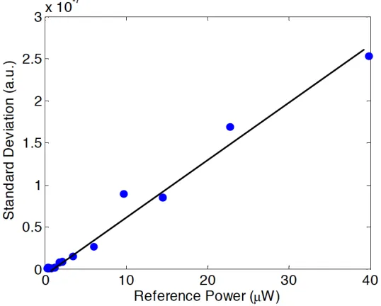
4.4.4 1/f Noise Power Dependence ...65
4.4.5 Sources of 1/f Noise...66
4.5 Conclusions ...67
Chapter 5. Dark 1/f Noise in Direct Detection Schemes...70
5.1 Introduction ...70
5.2 Background ...73
5.3 Problem Statement ...75
5.4 Experimental Verification...77
5.5 Theory ...78
5.6 Results ...83
5.7 Discussion ...85
5.7.1 Summary of Analysis...85
5.7.2 Application of Analysis ...86
Chapter 6. 1/f Noise in FDOCT ... 90
6.1 Introduction... 90
6.2 SNR of M-mode Data... 92
6.3 SNR of FDOCT Images ... 96
6.4 Conclusions... 98
Chapter 7. Turbidity Suppression Through Optical Phase Conjugation ... 99
7.1 Optical Phase Conjugation ... 99
7.1.1 OPC Based on Static Holography... 100
7.1.2 OPC Based on Dynamic Holography Through Degenerate Four-Wave Mixing ... 103
7.2 Previous Work ... 104
Chapter 8. TSOPC System Characterization... 107
8.1 Introduction... 107
8.2 Materials and Methods ... 109
8.3 Results... 112
8.3.1 Chicken Breast Tissue Experiments ... 112
8.3.2 Tissue Phantom Experiments... 115
8.3.3 Resolution Trends ... 116
8.4 Discussion... 118
8.4.1 Amplitude Trends in Tissue Samples ... 118
8.4.2 Amplitude Trends in Tissue Phantoms... 120
8.4.4 Resolution Trends ...124
8.4.5 Significance and Future work...126
8.5 Conclusions ...127
Chapter 9. TSOPC in Living Tissues...128
9.1 Introduction ...129
9.2 Experimental Methods...130
9.3 Results and Discussion...132
9.4 Conclusions ...136
Chapter 10. Potential Applications and Future Work for TSOPC ...137
10.1 Potential Applications...137
10.1.1 Light Concentrating Applications ...137
10.1.2 Absorption Amplification Applications ...139
10.1.3 Wavelength Tuning for Light Selection...140
10.2 Future Work ...142
Chapter 11. Conclusions ...144
References ...145
Appendix D1: Chapter 3 Derivations ...155
D1.1 Derivation of Variance for Heterodyne Detection ...155
D1.2 Derivation of Variance for Heterodyne Detection with Phase Knowledge...156
D1.3 Derivation of Variance for Method 1 ...157
D1.5 Derivation of Variance for Method 3... 158
D1.6 Derivation of Variance for Method 3, n Ports ... 158
D1.7 Derivation of Variance for Methods 4 and 5 ... 159
List of Figures
Number Page
1.1 Therapeutic window in the optical absorption spectrum of tissue components... 3
1.2 Time-resolved light scattering in tissues... 4
2.1 Time domain OCT ... 14
2.2 Spectrometer-based Fourier domain OCT... 17
2.3 SNR as a function of reference arm reflectivity... 19
3.1 3x3 fiber-coupler-based homodyne optical coherence tomography ... 25
3.2 2x2 (50/50) interferometric setups... 28
3.3 Reconstructed signals from an attenuated mirror... 39
3.4 Reconstructed images of a highly attenuated Air Force target... 40
3.5 Reconstructed images of a Xenopus laevis tadpole ... 42
3.6 SNR versus phase error... 43
4.1 Influence of the total time frame, T, of an experiment ...53
4.2 Theoretical noise standard deviation versus integration time...55
4.3 Theoretical SNR versus integration time ...56
4.4 τ dependence of 1/f noise variance ...58
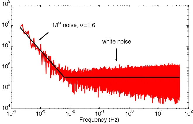
4.5 Power spectrum of interferometric noise ...61
4.6 Experimental SNR versus integration time ...62
4.7 Homodyne vs. heterodyne SNR...63
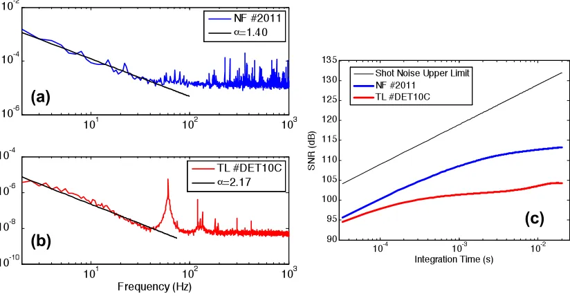
4.9 Power spectra and SNR for two types of detectors...67
5.1 A comparison of the measurement scenarios in Chapters 3 and 4 ...76
5.2 Power spectral density of the dark noise count of an APD...77
5.3 SNR versus integration time for a combination of white and 1/f noise...83
5.4 Dependence of τopt on the relative amplitudes of white and 1/f noise ...84
6.1 System schematic for common path FDOCT ...92
6.2 Power spectrum of the system noise...93
6.3 M-mode SNR as a function of time ...95
6.4 Image SNR as a function of integration time...97
7.1 A conventional mirror compared to a phase conjugate mirror ...100
7.2 OPC through static holography...101
7.3 Proof-of-concept TSOPC experiment...105
8.1 TSOPC system schematic ...111
8.2 Chicken tissue samples ...112
8.3 Experimental TSOPC amplitude data in chicken tissue samples ...114
8.4 Experimental TSOPC amplitude data in tissues phantoms...115
8.5 Focused beam sample arm geometry...116
8.6 Resolution trends for chicken tissue samples ...117
8.7 Resolution trends for tissue phantoms ...118
8.8 Model fits for both chicken tissue and tissue phantom data ...124
9.1 The ear of a New Zealand rabbit mounted in the TSOPC system ...131
phantom of comparable properties...132
9.3 TSOPC signal versus sample displacement during playback ...133
9.4 Histology of the rabbit ear ...134
9.5 Signal decay through the rabbit tissue ...135
10.1 Diagram depicting potential light concentrating experiments... 137
10.2 Diagram depicting potential absorption amplification experiments... 139
10.3 Diagram depicting wavelength tuning experiments ... 141
List of Tables
Number Page
1.1 Scattering and absorption properties of tissues...7
3.1 Comparison of theoretical and experimental reconstruction results...37
Abbreviations
APD Avalanche photodiode
CCD Charge-coupled device
DFWM Degenerate four-wave mixing
FDOCT Fourier domain optical coherence tomography
FWHM Full-width at half-maximum
FWM Four-wave mixing
NA Numerical aperture
OCT Optical coherence tomography
OPC Optical phase conjugation
PMT Photomultiplier tube
PrC Photorefractive crystal
PSD Power spectral density
sFDOCT Spectrometer-based Fourier domain optical coherence tomography
SLD Superluminescent diode
SLM Spatial light modulator
SNR Signal-to-noise ratio
TDOCT Time domain optical coherence tomography
Chapter 1. Introduction
1.1 Advantages and Challenges Associated with Optical Imaging
Optical methods are uniquely suited to biological imaging for several distinct reasons. The
contact nature of light delivery provides for an extremely invasive and
non-destructive imaging modality that can be implemented at relatively low cost. Second,
optical techniques are generally capable of providing resolution on the order of the
wavelength of light. This provides for high-resolution (sub-micron) cellular and tissue
level imaging. Finally, the energy quanta associated with visible and near infrared photons
are ideal for interacting with biological molecules. Such molecular interactions provide the
basis for techniques including fluorescence, multi-photon microscopy, second harmonic
generation, and Raman spectroscopy, allowing for functional or molecule-specific imaging
of biological tissues. Thus, light can provide for non-contact, high-resolution, functional
imaging of biological features of interest.
The advantages of optical techniques are accompanied by significant challenges.
Some of the above-mentioned techniques rely on a photon being absorbed by a molecule of
interest. However, as we will see in the following sections, absorption is dominated in
tissues by elastic light scattering. In a biological environment, a photon is hundreds to
thousands of times more likely to be scattered than absorbed. This presents a problem for
biological imaging, even for optical techniques that rely in part on light scattering for
contrast. As photon trajectories become increasingly complicated, it becomes impossible
1.2 Optical Properties of Tissues
1.2.1 Absorption
Absorption occurs when energy is transferred from light to a molecular species. During
this process, the molecular species transitions from a lower to a higher energy level, where
the difference in energy between the two levels, ΔE, is equal to the energy of the photon,
hυ:
hυ = ΔE, (1.1)
where h is Planck’s constant (6.626x10⁻³⁴ Js), and υ is the optical frequency (light is defined as the portion of the electromagnetic spectrum with frequencies υ = c/λ= 3x10¹⁴ to 3x10¹⁵, where c is the speed of light). From an excited state, the molecular species can release this energy as either heat or in the form of a secondary photon (fluorescence,
phosphorescence), or transfer the energy to a neighboring molecule.
Absorption can be quantified through several parameters. For a single type of
absorber, the absorption cross section is defined as:
Pa = I0σa, (1.2)
where Pa is the absorbed power (energy per second) and I0 is the intensity incident on the
absorber (energy per second per area). The absorption cross section, σa, is a measure of the
area of an incident beam that is absorbed by an absorbing particle, and is generally not
equal to the geometric cross section of the particle. If many identical particles exist in an
absorbing medium, that medium can be characterized by an absorption coefficient:
µa = ρaσa , (1.3)
where ρa is the number density (number per unit volume) of the absorbers. The absorption
la = 1/µa , (1.4)
which is a measure of the average distance an individual photon will travel through the
medium before being absorbed. The Beer-Lambert law makes use of the absorption
coefficient to describe the intensity decay through an absorbing medium (1):
I(x) = I0exp(-µax), (1.5)
where I0 is the intensity at x=0.
There are many important absorbers in tissues including water, hemoglobin,
melanin, and many others. Figure 1.1 shows the absorption spectrum of some of these
important tissue chromophores, as both σa and µa are functions of wavelength. The
majority of optical imaging techniques work in the ‘therapeutic window’ from 600 to 1300
nm (1). This window is bounded by the large absorption of hemoglobin and water on
either side. However, within this window, absorption effects are relatively small compared
to scattering effects, which we will discuss in the following section. Absorption is
diagnostically important for many routine optical techniques such as pulse oximetry and
angiography.
1.2.2 Scattering
The second major process by which light interacts with tissues is through light scattering.
Similar to absorption, a scattering cross section can be defined for a single, spherical
scatterer as:
Ps = I0σs, (1.6)
where Psis the power of the light that is spatially redirected through scattering. Again, σs is
not necessarily equal to the geometric cross section of the scatterer. For a uniform medium
of particles, a scattering coefficient and mean free path can be defined as in Eqs. 1.3 and
1.4, and Beer’s law holds true as well:
Iballistic(L) = I0exp(-ρsσsL) = I0exp(-µsL). (1.7)
Instead of the total intensity exiting the medium, the left hand side of Eq. 1.7 is a measure
of the intensity of the unscattered, or ballistic, light component.
If a pulse of light is incident on a scattering medium or slab of tissue, the exiting
photons can be divided into three main components (illustrated in Fig. 1.2). The first to
exit the material is the ballistic component, with intensity given by Eq. 1.7. These photons
Figure 1.2. Time-resolved light scattering in tissues
!"#$%&"'()*+,&(
-#./&0$"1(2&%$.(
-).#&( 3$4*,&(
have traveled straight through the medium. A second component, consisting of ‘snake’
photons, forward scatter through the medium along an approximately straight path. These
are the first of the scattered photons to leave the medium. Finally, the bulk of the light is
diffusely scattered, having followed a tortuous path through the medium.
Due to the phenomenon of multiple scattering, Eq. 1.6 cannot be generalized for a
medium containing N scatterers except under specific approximations (1). The total power
scattered by a scattering media can be written as:
Ps = AI0(1-exp(-µsL)) ≈ AI0ρsσsL = I0Nσs , (1.8)
only if µsL << 1. Thus, for a weakly scattering medium, the scattered power is proportional
to the number of scatterers. However, when this approximation breaks down, more
complicated methods and models must be used to accurately predict the diffuse scattering.
Two types of scattering events are possible (3). The vast majority of scattering
events are elastic, meaning that no energy is transferred between the light wave and the
particle; the light is simply redirected spatially. Alternatively, for a small fraction of
scattering events (1 in 106 (1)), inelastic or Raman scattering occurs and the scattered wave
undergoes a frequency shift that is specific to the molecular composition of the scatterer.
Raman spectroscopy has a wide range of applications through its ability to study
molecule-specific vibrational and rotational modes.
A final parameter of interest is the scattering anisotropy factor, g. This factor,
defined as the average cosine of the scattering angle (g=<cosθ>), is a measure of the
angular spread of scattering distribution. A g value close to 1 implies a high level of
forward scattering, while a g value close to 0 corresponds to a nearly isotropic scattering.
1.3 Typical Methods to Deal with Light Scattering
Table 1.1 confirms that tissue scattering is quite strong. Thus, imaging through tissues
requires effective methods for dealing with light scattering. In both the Mie and Rayleigh
regimes, light scatters more strongly at shorter wavelengths. Therefore, one way to
minimize scattering is to work at longer wavelengths. There is a limit, however, since Fig.
1.1 shows that water begins to absorb strongly for wavelengths longer than ~1300 nm.
Two broader strategies will be discussed in this section: gating methods and diffuse optical
methods.
1.3.1 Gating Methods
Several optical imaging techniques rely on methods to filter out ‘information
bearing’ ballistic or singly scattered photons from the large number of multiply scattered
photons that exit the tissue. These include time, directional, and coherence gating (as used
in optical coherence tomography). Time gating techniques make use of the fact that
ballistic and snake-like photons exit the scattering media at an earlier time than diffuse
photons (Fig. 1.2), and can thus be filtered out appropriately. This can be accomplished
using fast electronics such as gated optical image intensifiers (8) or holography with
femtosecond pulses (9). Additionally, more complex schemes have involved the use of
nonlinear optical effects (10, 11) or stimulated Raman scattering (12).
Alternatively, directional gating rejects light whose propagation direction has been
sufficiently altered by light scattering. For example, a confocal microscope detects only
portions of the transmitted or reflected light that pass through a pinhole. This not only
different position than the pinhole), but also rejects the bulk of the multiply scattered light.
This type of gating technique is not particularly selective to the ballistic component of the
light, since the snake-like components travel in approximately the same direction as the
ballistic component.
Finally, another commonly used gating method is coherence gating. Coherence is
the property of a wave that allows for interference, and can manifest either temporally or
spatially. Perfect coherence implies a constant relative phase between two waves, meaning
that a perfectly temporally coherent wave is monochromatic. A source with a given
spectral bandwidth is said to be partially coherent, since as the waves propagate over time
or space, the phase relationship between individual frequencies will change. This is useful
in an interferometric setting where a sample beam is interfered with a reference beam. For
a partially coherent source, a strong interference signal is only seen when the sample and
reference path lengths are exactly matched, and all frequency components are in phase.
With the reference path length appropriately set, coherence gating employs a partially
coherent light source to select for the light component that has traveled straight through the
sample. This topic will be discussed in detail in Chapter 2.
Since the probability of finding ballistic or singly scattered photons decreases
exponentially with depth into the sample (Eq. 1.7), these gating techniques suffer from
limited penetration depths due to scattering. They rely on systems that operate at very high
signal to noise ratios (SNRs) to measure the weak signal contribution from within tissue
samples. Even with high SNR, these systems are generally limited to a penetration depth
1.3.2 Diffuse Optical Methods
An alternate method for imaging into scattering media involves collecting all of the
diffuse photons shown in Fig. 1.2. In these methods, wave effects such as polarization and
interference are neglected, and only energy flow through the medium is tracked. Radiation
transport theory provides a model to characterize light energy propagation based on three
parameters: absorption and scattering coefficients, and a scattering phase function (1). The
scattering phase function describes the angular profile of the scattered light. Several
approximations exist that are functions of the anisotropy factor, g (13). In the diffusion
limit (when absorption is significantly weak), the scattered light disperses in a seemingly
random fashion throughout the medium, appearing to take a random walk defined by the
diffusion equation. Numerically, these types of computations can also be performed using
Monte Carlo methods in which random numbers are drawn from probability distributions,
corresponding to average optical properties, to model random walks through a given media
(14, 15).
The above methods can be employed for depth resolved imaging through diffuse
optical tomography (DOT). This is a difficult endeavor, because it involves solving an
ill-posed inverse problem to determine the distribution of the optical properties of a sample
based on the measured scattering. Typically a pulse of light enters the sample at a
particular source location, and the scattered light is measured at an array of detectors.
Then, the source location is moved and the process is repeated. A great deal of information
is acquired, and the solution to the forward problem is applied iteratively to an estimate of
the sample optical property distribution until the output matches the measured data. Since
than the coherence domain techniques mentioned above (several cm at 700 nm (3)).
However, in general, DOT is a low-resolution technology with spatial resolution on the
order of 20% of the penetration depth (3). DOT has been applied for both breast and brain
imaging (16–18), but resolution remains a fundamental limitation.
1.4 Goals and Layout of the Thesis
Taking the above discussion into account, the question remains: how can we optimize
optical imaging in biological samples? The work presented in this thesis will describe two
main approaches. First, assuming nothing can be done about strong scattering, we can
optimize our systems to run with a high signal-to-noise ratio (SNR), making it easier to
pick up the weak signal contribution from light that has scattered deep within the sample.
Since most of the systems that we will discuss in terms of optimization fall into the
category of coherence domain systems, the following chapter will provide background
materials on coherence domain imaging. Chapters 3, 4, and 5 include experiments and
results that are adapted from published manuscripts, while Chapter 6 is adapted from an
as-of-yet unpublished manuscript. Chapter 3 describes SNR optimization based on image
processing algorithms for an interferometric system based on the phase shifts inherent to a
3x3 fiber coupler. Chapter 4 discusses the impact of 1/f noise on the same system, and
develops a generalized model that accounts for the effects of 1/f noise with the goal of
allowing a user to select appropriate operating parameters to achieve optimal SNR.
Chapter 5 discusses the adaptation of that model to direct detection schemes, and finally
Chapter 6 discusses its application for Fourier domain optical coherence tomography
The thesis changes directions in Chapter 7 to discuss a second approach for
optimizing optical imaging, a novel technique termed turbidity suppression through optical
phase conjugation (TSOPC). Through this technique, we attempt to time reverse the
process of elastic light scattering in order to recover information about the incident wave.
Chapter 7 serves as background for the remainder of the thesis, describing the
fundamentals of phase conjugation as well as preliminary work in applying phase
conjugation to biological tissues. Chapter 8 is a stand-alone manuscript that has been
submitted for publication, which describes a detailed characterization of the TSOPC
experiment in terms of amplitude and resolution trends. Chapter 9 discusses a set of results
concerning TSOPC in living tissues. Chapter 10 discusses the potential value of our work
on TSOPC in terms of biomedical applications. Finally, Chapter 11 will draw brief
Chapter 2. Background on Coherence Domain
Imaging Systems
This chapter is intended to provide background information for Chapters 3–6, as several of
the systems that will be discussed fall into the category of coherence domain imaging
systems.
2.1 Optical Coherence Tomography
2.1.1 Time Domain OCT
Optical coherence tomography (OCT) is an increasingly popular imaging modality capable
of non-invasively providing depth-resolved images of biological structures with
micron-scale resolution in real time (19). OCT is a form of low coherence interferometry, which is
based on coherence gating (as briefly described in Section 1.3.1).
A standard, fiber-based, Michelson-type interferometer is depicted in Fig. 2.1(a).
Light entering the interferometer is split into two optical paths at a fiber coupler (the fiber
equivalent of a beamsplitter). One light path reflects off of a mirror, while the other probes
the sample. The two returning light fields are then recombined and interfere at a
photodetector. In a time domain implementation of OCT, the reference arm is scanned in
time. Let us, for a moment, discuss the detected signal for the case with a mirror as the
sample, and a monochromatic light source. In this case, as the reference arm is scanned,
the two beams alternately constructively and destructively interfere to form a fringe pattern.
where NA is the numerical aperture of the focusing and collection optics, f is the focal length, and D is the diameter of the collimated beam that is focused onto the sample. The spot size varies with depth into sample as follows:
€
w
( )
Δz =w0 1+ λ0Δzπw02
, (2.5)
where Δz is the axial distance from the minimum beam waist. A relatively low level of
focusing is typically employed to limit beam divergence throughout the imaging depth.
If the reference arm in a TDOCT system is capable of moving to any arbitrary
distance, then the maximum imaging depth is limited by scattering based on the SNR of the
system. The SNR of these types of systems will be discussed in detail in Section 2.1.3.
2.1.2 Fourier Domain OCT
Within the last 10 years, the OCT community realized that there is an alternate way of
acquiring the same information. Fourier domain implementations of OCT (FDOCT)
sample the interference pattern as a function of wavenumber (k), with a fixed reference path length. A depth scan into the sample is then obtained by Fourier transformation. This
can be accomplished in two ways. Spectrometer-based FDOCT systems utilize a
spectrometer to spectrally disperse light in the detection arm of the interferometer over a
CCD (Fig. 2.2(a)). Alternately, swept source FDOCT systems use a wavelength swept
laser source, such that the spectral interferogram is obtained at a single photodetector as a
function of time. Spectral encoding can be described in a form similar to Eq. 2.2 as:
€
where ρ is the detector efficiency (typically assumed to be uniform across k) and S(k) is the source power spectral density in units of watts per wavenumber. Thus, the detected signal
at the spectrometer is the source spectrum modulated by interference fringes as shown in
Fig. 2.2(b). Fourier transformation of this spectrum results in the same depth scan found
after demodulation of the detected TDOCT signals. A Fourier domain implementation is
not only advantageous due to the fact that it does not require a moving reference arm, but it
also provides an SNR advantage (22–24) due to the fact that information is collected from
all depths simultaneously (i.e., none of the incident light is wasted).
Figure 2.2. Spectrometer-based Fourier domain OCT. a) system schematic. b) detected signal on CCD camera
In FDOCT systems, the maximum imaging depth is fundamentally limited. As
mentioned above, the depth scan of the sample is obtained from a Fourier transform of the
interferometric portion of the detected signal as a function of wavenumber. The maximum
depth is determined by the highest frequency on the spectrum that can be resolved by the
!"#$
!%#$
system. For a spectrometer-based system this is a function of the δλ or δk that corresponds
to one spectrometer pixel. For a swept-source system, this is determined by the frequency
step that occurs over a single time step.
2.2 Common Noise Sources and SNR Optimization
The maximum detected signal in an OCT system, for a single path-length matched
reflector, is given by:
€
Pdetected, max =PS +PR +2 PSPR . (2.7)
The term of interest is the third term, which was the coefficient of the cosine term in Eqs.
2.2 and 2.6. It can be isolated through appropriate subtraction of the DC terms, however
noise from these terms will remain. In order to achieve high quality images, we are
interested in how the signal term compares to system noise.
The typical noise sources considered in OCT imaging are white noise sources,
which include receiver noise, shot noise, and excess intensity noise (25). Receiver noise
generally has both white and colored components. The white component is due to Johnson
noise in the system circuitry caused by thermal agitation of charge carriers (26, 27). Shot
noise is inherent to any beam of light, and is caused by the Poisson distributed arrival time
of individual photons. Finally, excess intensity noise is caused by polarization fluctuations
in the light source and generally scales with intensity (28). Figure 2.3, from Ref. (25),plots
the OCT signal-to-noise ratio (SNR) expected when each of these three noise sources is
dominant (inversely proportional to the level of noise). It is typical to optimize OCT
systems by adjusting the reference arm power to sit in the shot noise limit. In this case the
limitations in increasing the power at the sample, since there are standards for living tissue
to prevent damage to the sample (29). It is less obvious that there are also limitations on
increasing the integration time due to the presence of non-white noise sources, specifically
1/f noise. We will discuss the effects of these limitations in the following chapters.
Briefly, the SNR advantage of FDOCT systems stems from the fact that signal is
collected from all illuminated depths simultaneously. For a TDOCT system that collects a
signal over N depth steps, only a fraction of the light reflected from the sample will be
capable of interfering with the reference signal and recorded. This fraction is given by
PS/N, and would serve to reduce the SNR by a factor of N in Eq. 2.8.
2.3 Extensions of Traditional OCT
A number of extensions of traditional OCT have been reported. These include polarization
sensitive OCT (30, 31), spectroscopic OCT (32, 33), molecular contrast OCT (34–36),
Doppler OCT (37), endoscopic OCT (38, 39), and phase-resolved OCT (40–42).
Here, we will provide a brief conceptual description of a specific extension of OCT
that will be discussed extensively in this thesis in the context of noise optimization: 3x3
fiber-coupler based homodyne en face OCT. First, the term en face refers to imaging in the transverse plane, perpendicular to the imaging beam, as opposed to in depth. En face
images can be produced from 3D volumetric OCT scans by collecting the data points that
correspond to a single depth, or, they can be acquired directly. In the 3x3 system, they will
be acquired directly. To produce en face scans, we essentially employ a TDOCT system with a stationary reference arm (corresponding to one particular depth place), and scan the
A standard TDOCT system is heterodyne in nature. A fringe pattern is produced as
the reference arm is scanned, and AC lock-in detection is performed to isolate the envelope
of interest. If the reference mirror is stationary, the system is converted to homodyne
system, since we no longer acquire full interferometric fringes. The difficulty in
performing direct detection of an interferometric signal is that we are unaware of the phase
of the signal that we are acquiring, making it impossible to determine the amplitude of the
signal through a single measurement. This particular system employs a 3x3 fiber coupler,
as the output of the 3 ports are phase shifted 120° from one another. By simultaneously
detecting these three signals, we can determine the amplitude of the OCT signal to form an
Chapter 3. Algorithms for Optimizing SNR
This chapter is adapted from Ref. (43): E.J. McDowell, M.V. Sarunic, Z. Yaqoob, and C. Yang, ‘SNR enhancement through phase dependent signal reconstruction algorithms for phase separated interferometric signals,’ Optics Express, 15(16), 10103–10122 (2007).
3.1 Introduction
There are a number of signal acquisition scenarios that involve the measurement of phase
separated components, such as quadrature components, that are later recombined in an
appropriate manner to extract phase and amplitude information. There are several reported
methods by which this extraction can be performed. Interestingly, the choice of signal
reconstruction algorithm can have a dramatic impact on the signal-to-noise ratio (SNR) of
the resulting image or signal.
Experimental designs in which phase separated components are detected include
phase shifting interferometry, optical gyroscopes, harmonic gratings-based free space
quadrature interferometers, and 3x3 fiber coupler-based homodyne interferometers. Phase
shifting interferometric techniques introduce small phase delays in the form of
subwavelength optical path length changes (44, 45). These phase shifted signals can then
be used to retrieve phase and amplitude information. In an optical gyroscope, light beams
traveling in opposite directions around a rotating path experience slightly different path
lengths due to the Sagnac effect (46). The intensity and phase retrieved from the resulting
phase shifted signals can be used to determine the rotation rate (47, 48). Harmonically
interferometry (49, 50). In such setups, the interference patterns between various
diffraction orders of the two gratings are acquired at multiple detectors. The harmonic
relationship between the gratings results in phase separation between the detected signals
that is non-trivial. The sensitivity of each of these techniques can benefit by recombining
the phase separated components in such a way that the total noise is minimized.
In the case of a 3x3 fiber coupler-based system, the intrinsic, nominally 120°,
phase shifts between ports of the fiber coupler can be used to decouple phase and
amplitude information (51, 52). These phase shifts arise due to evanescent coupling
between fiber waveguides as described by coupled mode theory (53, 54), or more simply
for 2x2 and 3x3 fiber couplers through conservation of energy (52). 3x3 fiber
coupler-based systems have been employed to construct homodyne en face OCT images of biological samples (51) and to remove the complex conjugate ambiguity in swept source
OCT images of the ocular anterior segment (55, 56). The simplicity of homodyne systems
compared to their heterodyne counterparts is a significant implementation advantage. In
addition, a properly performed homodyne experiment can provide a 3 dB improvement in
SNR compared to heterodyne techniques (57–59).
Quadrature components are also commonly detected in signal acquisition
schemes for other biomedical imaging techniques, such as nuclear magnetic resonance
(NMR), magnetic resonance imaging (MRI), and Doppler ultrasound. Like the
abovementioned optical techniques, these signals must also be recombined in order to
retrieve amplitude and phase information. NMR spectrometers commonly utilize two
detectors, acquiring 90° phase shifted signals to allow for improved pulse power efficiency
systems are combined for phase or amplitude imaging. The MR community is well
aware that the SNR of the resulting images is affected by the way the image is
reconstructed (61–63). Finally, in Doppler ultrasound systems the real and imaginary parts
of the Doppler shift signals are detected in order to determine amplitude and phase, which
is necessary to determine Doppler information (64).
In this chapter we will report on the SNR advantage that can be achieved by
recombining phase separated signals in an optimal manner. Our goal in each of the
reported signal reconstruction algorithms is to determine the amplitude of the signal as
accurately as possible. In the process we may or may not determine the phase of the
signal as well. That said, we find that methods that make use of the phase information
contained in the measurements perform better than those that do not. In Section 3.2 we
will describe our 3x3 fiber coupler-based homodyne OCT system. We will then describe
five different image reconstruction algorithms in Section 3.3, including two
phase-dependent methods. We theoretically determine that these algorithms achieve improved
SNR as compared to the other three reconstruction methods, and find that they are capable
of achieving comparable SNR to commonly employed heterodyne techniques. Notably,
these algorithms are not specific to our 3x3 fiber coupler-based OCT system, but are
general techniques applicable for use in signal extraction processing wherever phase
separated components are available. In Section 3.4 we will describe our experimental
setup. In Section 3.5 we compare our experimentally determined SNR values to those
derived in Section 3.3, and discuss the influence of the five methods on reconstructed
Figure 3.1. 3x3 fiber-coupler-based homodyne optical coherence tomography. a) experimental setup. SLD: superluminescent diode, Dn: nth photodetector, M: mirror, X-Y: x-y scanner, OBJ: 20x microscope objective. b) In this homodyne system the reference mirror (M) is stationary. We can think of the measured signal as a single point (black arrow) on the modulated coherence function that would be obtained if the reference arm was swept. c) These points are the projections of a complex value onto axes separated by 120°.
3.2 3x3 Homodyne OCT Theory
We will first describe the 3x3 homodyne OCT system for high-resolution en face imaging of biological samples (following Ref. (51)). This scheme has the ability to decouple
amplitude and phase information without the need for complex rapid scanning optical
delay mechanisms used in heterodyne systems, or expensive components such as
spectrometers or swept laser sources. Figure 3 . 1(a) shows the experimental setup
utilized in this study. Broadband light from an SLD (λ0=1300 nm, Δλ=85 nm) enters a
create an interference pattern at detectors 1–3. Detector 4 is used to monitor and
correct for source fluctuations. Figure 3.1(b,c) diagrams the type of data that we are
collecting. Using a stationary reference arm, we are essentially measuring a single point on
the interferogram (represented by the thick black arrow, Fig. 3.1(b)). Thus, we
measure three interferometric signals that can be thought of as the projections of a
complex signal onto axes separated by 120º (Fig. 3.1(c)). The optical signal at the jth
detector is given by
€
Pj
( )
z =Pr,j+Ps,j+2 1 sj( )
α41α4jα51α5jPr(
PS( )
z ⊗γ( )
z)
cos(
θ( )
z +ϕj)
. (3.1)where Pr,j and Ps,j represent the total DC power returning from the reference and sample arms, respectively; 1/sj is a scaling factor that accounts for both coupler and detector loss;
Pr is the returning reference power; Ps(z) is the returning coherent light from a depth
z within the sample; γ(z) is the source autocorrelation function; θ(z)=2k0z+ψ(z), is the
phase associated with each depth in the sample, where k0 is the optical wavenumber
corresponding to the center wavelength of the source and ψ(z) is the intrinsic reflection
phase shift of the sample at depth z; Finally, ϕj represents the phase shifts between each of
the three detectors, attributable to the intrinsic phase shifts of the 3x3 fiber coupler. The
signal of interest, which describes the reflectivity profile of the sample, is the coefficient
of the cosine term, which can be isolated in several ways following removal of the DC
terms. Below we describe several techniques to reconstruct the coefficient of the cosine
term.
3.3Theoretical SNR Corresponding to Image Reconstruction Algorithms
reconstruction algorithms. For comparison, we will also derive the SNR corresponding to
both optimal and commonly employed homodyne and heterodyne techniques. In each of
the following derivations we will make the assumption that the signal at each detection
port in terms of number of detected photons, is given by:
€
Si =2
n PRPS
ετ
hυcos
(
θ+ϕi)
±Ni, (3.2)where PR and PS are the power returning from the reference and sample arms,
respectively, n is the number of detection ports (n≥2), ε is the detector quantum
efficiency, τ is the integration time, h is Planck’s constant, and υ is the optical frequency.
Ni represents a fluctuating noise term that is zero mean, and assumed to be Gaussian
distributed with standard deviation as expected given shot noise limited detection:
. (3.3)
Finally, we assume that the optical power returning from the reference arm is much
greater than that returning from the sample arm (PR>>PS), which is typical when imaging
highly scattering biological samples. In Eq. 3.2 we have assumed that the terms Pr,j and
Ps,j from Eq. 3.1 have been subtracted. This can be accomplished in a practical setting by
alternately blocking the sample and reference arms to measure their individual
contributions.
In each of these reconstruction methods we wish to isolate a signal that is
proportional to the power returning from the sample, PS. Thus, our goal is to isolate the
square of the coefficient of the cosine term in Eq. 3.2. In addition to this signal, we will
also determine how the reconstruction method affects both the expected value and
in image quality. The standard deviation of the noise is related to the SNR, which
determines the lowest amplitude features that are visible in the image. The expected, or
mean, value of the noise can add a DC shift to the image, thereby affecting the contrast of
the image.
Figure 3.2. 2x2 (50/50) interferometric setups utilizing a) homodyne and b) heterodyne detection. In (a) the reference mirror is stationary, while it is translated in (b). The 180° phase shifts of the fiber coupler are evident in the acquired signals at the two output ports.
3.3.1 Optimal SNR in Common Interferometric Topologies
Here we describe the theoretical SNR corresponding to common interferometric setups.
Figure 3.2 shows schematics of the setups that we will examine, which include 2x2
(50/50) fiber coupler-based Michelson interferometers employing a) homodyne and b)
heterodyne detection. The signal and noise at each output port of the coupler can be
represented by Eqs. 3.2 and 3.3 where n=2 to account for the power splitting ratios of the
50/50 fiber coupler.
The upper limit on SNR can be achieved in a homodyne experiment with perfect
Knowledge of phase can be attained in two ways. In the first situation, the phase is
known prior to the measurement. This scenario can conceivably occur in well-controlled
experiments where the only unknown variable is the signal amplitude. In the second
situation, an estimate of the phase can be extracted from the measurement itself, and that
information is then used in computing the signal amplitude. This type of phase estimation
is employed in some of the following signal reconstruction algorithms. We note that the
computation of signal amplitude where phase knowledge is used can be expected to be less
robust and prone to systematic errors. In Section 3.5.3, we investigate the effect of phase
error on our signal reconstruction algorithms, and find that they are surprisingly robust.
Heterodyne detection is typically accomplished using an AC lock-in amplifier. The
measured signal is multiplied by a sine and cosine oscillating at the signal frequency, and
summed over a variable time step, τ. The two outputs of the lock-in provide quadrature
components for determination of signal amplitude and phase. The amplitude of the signal is
then computed as the magnitude of the quadrature components. The signal reconstruction
process can be written as the following, where S is the measured data:
. (3.9)
The time step for each term in the summation is τ/X. In an analog mode lock-in amplifier X
is effectively infinity and the summation can be replaced by an integration. As we shall see,
the actual value of X (as long as it is >2) has no impact on the computed SNR. For the
purpose of comparison, this method and each of the following methods leads to a
reconstructed signal that is identical to Eq. 3.5. Derivation of the expected value and
variance of the noise for this and following methods is detailed in Appendix D1. The
3.3.2 Method 1
Here we begin to discuss methods for image reconstruction given phase separated
components at the three ports of a 3x3 fiber coupler based OCT system. We assume ideal
conditions in which the power splitting ratios for the coupler are equivalent (αij=1/3),
φj=120°, and si=1, and the signal and noise at each point is given by Eqs. 3.2 and 3.3
where n=3.
The most common method to reconstruct an image is to simply square and sum
the signals from each port of the fiber coupler (51). This processing removes the cosine
terms, which contribute a factor of 3/2 to the final reconstructed signal. We define
method 1 as follows:
. (3.17)
We can determine the mean value and variance of the noise to be:
€
E M
[
1( )
Ni]
=9 2σ2 (3.18)
€
σM 1 2
=27 2σ
4, (3.19)
and find an SNR of:
. (3.20)
3.3.3 Method 2
A second method takes advantage of instantaneous quadrature, as described by Choma et
al. (52). Taking the signal at port 1 of the coupler, S1, as our real signal, the imaginary
Scaling factors, ai, are determined by substituting the measured phases, as well as φi, and
minimizing the resulting noise. For example, if the values of θ andφi for a given channel
produce a cosine value close to zero, then the noise would increase greatly after dividing
it by this small number. Hence, this channel would be weighted the least compared to the
others. And conversely, maximally interfering signals (large cosine value) are weighted
more heavily than others. Since the noise in each channel is equivalent, larger
interferometric signals should lead to an increase in SNR. The values of the scaling
factors can be expressed as a function of the phase as well as the phase shifts between
subsequent ports:
€
ai =2 3 cos
2
θ+ϕi
(
)
[
]
. (3.27)The noise parameters and SNR that correspond to this method are:
€
E M
[
3[ ]
Ni]
=32σ2 (3.28)
€
σM3 2
=92σ4 (3.29)
. (3.30)
This method can be generalized for an nxn fiber coupler based interferometer. In this
case, the reconstruction based on Method 3 is given by:
, (3.31)
The results of these derivations can be found in Table 3.1. We note that the two
methods that incorporate phase information, Methods 3 and 5, are predicted to have
better SNR in comparison with the other methods. It is interesting to note that Methods 3
and 5 are predicted to have the same SNR. In fact, as is derived in Appendix D1, a
substitution of Eq. 3.32 for ai converts Method 3 into a form identical to Method 5.
However similar, we note that these methods differ in the case where the phase shifts at
the ports of the fiber coupler are not equally spaced (i.e., φi≠ 2π(i-1)/n). In this case, the
ais can be determined through a minimization, and the method will produce an image
with a different SNR than that derived above. Method 5 requires that the phase shifts be
equally spaced, and will not perform well under these conditions.
Finally, we note that although we have assumed shot noise limited detection in
these derivations, the five methods will perform the same with respect to one another so
long as the dominant noise source is white.
3.4 Experimental Methods
The system depicted in Fig. 3.1 was calibrated to determine accurate values for φi and si.
In order to make SNR measurements, a mirror was placed in the sample arm to serve as
an ideal reflector, which was attenuated (-70 dB) such that sample arm shot noise was
negligible compared to that from the reference arm. A beam chopper was used to
alternate measurements of signal and background noise. In order to assure that we were
using our homodyne system to acquire shot noise limited data, as opposed to dominant
1/f noise, we sampled quickly, at 800 kHz, and limited our data averaging time (~0.65
ms) following the results of Ref. (65). Both signal and noise data were reconstructed
using the five methods described above, and the SNR was determined as the mean signal
divided by the standard deviation of the noise. The methods were also compared based
on the mean value of the reconstructed noise.
We then used the 3x3 homodyne OCT system to acquire several images. Our system
resolution has been measured to be approximately 14 µm in the axial direction, and 9.4
µm in the lateral direction. First, we imaged a highly attenuated Air Force test target (-50
dB) in order to visualize the relative performance of the three methods in a low signal
situation. We then imaged stage 54 Xenopus laevis tadpoles. Each data set was processed using the five image reconstruction algorithms described above, and displayed on
equivalent color scales. The improved image contrast obtained using reconstruction
Figure 3.3. a) Reconstructed signals from an attenuated mirror. A beam chopper was used to make measurements of both signal and background noise, which were used to experimentally determine the SNR of the five methods. b) A magnified view of the noise from (a) depicting experimentally determined values for the mean and variance of the noise.
3.5 Results and Discussion
3.5.1 Experimental SNR Results
We evaluated our reconstruction methods based on data acquired with an attenuated mirror
in the sample arm. Figure 3.3 displays a typical reconstructed trace, showing alternating
signal and noise measurements as the sample beam was chopped. The SNR of the
reconstructed signals were determined, as well as the mean value of the noise. Both
1, showing that Methods 3 and 5, which take advantage of the known phase in order to
minimize the noise, perform significantly better than the other methods in terms of SNR. In
close agreement with our theoretical predictions, we found an SNR enhancement of up to
5.4 dB over the phase independent methods. These two methods also leave the smallest
remaining DC noise after signal reconstruction. However, we note that these two methods
do not match theoretical predictions for mean noise as closely as the other three methods.
It is reassuring that Methods 3 and 5 vary from theory in a comparable manner, since they
perform very similar processing; however, the exact cause of this discrepancy is unclear to
the authors at this time.
Figure 3.4. These images show a portion of a highly attenuated Air Force test target, representing a very low signal situation. The three images were reconstructed from a single data set and reconstructed using Methods 1–5 (described above). Methods 3 and 5 clearly perform better than the others, showing a notable increase in contrast between the bars of the test target and the background.
3.5.2 Imaging Results
The SNR improvement noted in the previous section is quite dramatic in our
reconstructed images. Figure 3.4 shows a portion of an Air Force test target. The
through the sample arm was very low. Each of the images shown in Fig. 3.4 was
reconstructed from the same raw data using Methods 1–5 described above. Additionally,
each image is displayed on the same color scale. We see that for the image reconstructed
using Method 2 the bars on the test target can barely be discriminated from the
background. The image reconstructed using Method 1 is better, but there is still
relatively little contrast between the bars and the background noise. As predicted by the
theoretical sensitivity analysis, Methods 3 and 5 produce images with a marked increase
in contrast compared to the others. The bars of the Air Force test target are clearly
distinguishable in panels (3) and (5) of Fig 3.4.
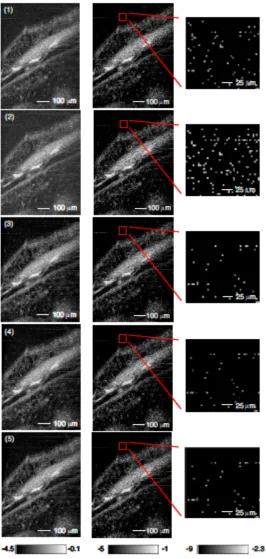
Our reconstruction algorithms were also tested on data from biological images.
Fig. 3.5 (first column) shows an image of structures in the anterior, medial portion of a
stage 54 Xenopus laevis tadpole. Again, Methods 3 and 5 produced images that more clearly distinguish biological structure from background noise. The nuclei of the cellular
structures at the bottom of the image are more visible. The ability to achieve superior
SNR based only on reconstruction algorithm implies that, to achieve the same SNR as
through commonly used reconstruction algorithms, the optical power incident on fragile
biological tissues can be reduced. In Fig. 3.5 (second column) we have subtracted the
DC value of the noise in each image in order to compare the noise variance between
images. When a portion of the background noise is magnified (Fig. 3.5, column 3), there
is significantly more background fluctuation in images corresponding to Methods 1 and 2
than in the other images.
We have seen in the above experimental results that Methods 3 and 5 are capable
each point in the image was used to minimize the noise at that point. In essence, these
algorithms utilize more of the available information than the other methods.
3.5.3 Robustness to Phase Error
The performance of each of the signal reconstruction methods depends on appropriate
calibration of the 3x3 homodyne OCT system. However, Methods 3 and 5 are strongly
dependent on correct calculation of the phase. Determination of the phase depends on
exact knowledge of the loss scaling coefficients, si, and the angles between adjacent ports
of the fiber coupler, φij. Uncertainty in these values leads to uncertainly in the phase at
various points in the image, and additionally leads to an improper choice of noise
minimization coefficients, ai, in Method 3. To reduce the effects of this potential
problem, we calibrated the 3x3 system immediately before image acquisition, making the
assumption that drifts in the system calibration parameters are slow.
Additionally, we investigated the impact of phase error on the SNR of the
reconstruction methods. To do this, we computed the SNR corresponding to each method
using a phase Θ+dθ, where dθ is a phase error that varies from 0 through π/2. The results
are plotted in Fig. 3.6 in terms of the SNR coefficient (i.e., the coefficient of PSετ/hυ).
The computation shows that Method 3 and 5 are surprisingly robust in the presence of
phase error. Very large phase errors may be incorporated before these methods drop
below the others in terms of SNR. These results imply that the phase-dependent methods
not only provide improved SNR, but are relatively insensitive to errors in system
calibration.
3.6 Conclusions
In conclusion, we have demonstrated the effect of image reconstruction algorithm on the
SNR when phase separated components are detected. We compared five potential
methods for reconstructing an image from the three outputs of a 3x3 fiber coupler-based
homodyne OCT system, and demonstrated that algorithms which use knowledge of the
phase at each point in the image to minimize noise perform significantly better than the
others in terms of SNR. This holds true for both homodyne and heterodyne techniques.
The algorithms showed an SNR increase of up to 5 dB over the other methods, and were
found to perform better than the most commonly used forms of heterodyne detection. This
increase in SNR was evident as improved contrast, as well as overall image quality, in
images from both an Air Force test target as well as biological samples. Additionally, we
found that these phase-dependent methods are relatively robust in terms of phase error.
applied to any situation in which phase separated components are combined to decouple
Chapter 4. Modeling the Effects of 1/f Noise
This chapter is adapted from Ref (65): E.J. McDowell, X. Cui, Z. Yaqoob, and C. Yang, ‘A generalized noise variance model and its applications to the characterization of 1/f noise,’
Optics Express, 15(7), 3833–3848 (2007).
4.1 Introduction
1/f noise, alternately referred to as pink or flicker noise, is found in a wide range of
physical systems (66–69), from carbon resistors and semiconductors (70), to heartbeat
dynamics (71) and traffic flow (72). In general, 1/f noise has a power spectral density that
follows the form 1/fα, where α commonly ranges from 0.5 to 1.5 (73). Despite significant
effort in describing a universal model for the origin of 1/f noise (74), no single model is
currently accepted, and the origins of 1/f noise have only been well characterized in very
specific circumstances. For example, 1/f noise in vacuum tubes is commonly modeled as
a superposition of relaxation rates that characterize the release of electrons from cathode
surface trapping sites (73, 75, 76). Additionally, the 1/f noise measured in cellular ion
currents has been attributed to the stochastic nature of the opening and closing
mechanisms of voltage gated ion channels (77).
The presence of 1/f noise in optical detection can significantly degrade the
effective precision and sensitivity of the optical technique. In interferometric methods,
including time domain optical coherence tomography (OCT) (19), a typical strategy for
is modulated and shifted into a frequency band in which 1/f noise is small compared to
other sources of noise. Under these circumstances, we typically consider only white noise
processes, which include receiver noise, shot noise, and excess intensity noise (25).
Homodyne methods are advantageous in their simplicity. By directly detecting the
interferometric signal, there is