Route choice modelling in dynamic traffic assignment

(1)

Peter Kant

Route choice modelling in

dynamic traffic assignment

(2)

Page i

Peter Kant

Route choice modelling in

dynamic traffic assignment

Master thesis

(3)

Page ii

Documentation page

Title report Route choice modelling in dynamic traffic assignment

Keywords Dynamic Traffic Assignment, Route choice modelling

Author Peter Kant

p.kant@alumnus.utwente.nl

Committee members Prof. Dr. Ir. E.C. van Berkum University of Twente Centre for Transport Studies e.c.vanberkum@ctw.utwente.nl

Dr. W. Kern

University of Twente

Discrete Mathematics and Mathematical Programming w.kern@math.utwente.nl

Drs. H.E. Mein

Omnitrans International emein@omnitrans.nl

Ir. D.H. van Amelsfort Goudappel Coffeng

dvanamelsfort@goudappel.nl

(4)

Page iii

Summary

Problem definition

Existing dynamic traffic assignment models become more and more advanced in terms of propagation, but in terms of route choice, many models are still pretty primitive. With the increase of research for route choice models, the question arises if it is possible to extend current propagation models by adding route choice to them. Questions included are which route choice models are good enough for application and how these models should be combined with the propagation model.

Methodology

In recent years, the research on route choice models and –more in general– discrete choice models from Random Utility Maximisation has increased significantly. Many research has been performed from a theoretical point of view. In this research the performance of several GEV based models is tested using a Monte Carlo (Probit) simulation technique. For this purpose a large scale network is used out of which 26 zones are selected for routeset generation, filtering and route choice calculation.

Additional research is performed to determine how route choice models and propagation models have to be combined. A new flexible dynamic equilibrium is presented to replace two existing dynamic equilibria (Boston & DUE). This equilibrium is formulated to better approach real traveller behaviour. A prototype model is developed and tested on a relatively small network.

Results and discussion

There are significant relations between characteristics of routesets and performance of the tested route choice models. This implies that the question which route choice models should be applied depends largely on the type of routeset. In general the PCL model gives relatively good results while not much effort has to be put in calibration.

(5)

Page iv

Conclusion and recommendations

It is possible to extend existing propagation models with route choice. The PCL route choice model is a good place to start, although also CNL, PSL and C-Logit give good results, depending on the characteristics of the routeset. If possible it is advised to determine which model to use before application.

The new equilibrium method using some kind of forecasting is assumed to be very powerful. It gives more flexibility than current instantaneous and dynamic equilibria.

(6)

Page v

Samenvatting

Aanleiding en probleemstelling

Bestaande dynamische toedelingsmodellen worden steeds geavanceerder op gebied van propagatie, maar zijn vaak nog erg beperkt in de routekeuze. De vraag die aan de basis van dit onderzoek ligt is hoe routekeuze op een juiste manier aan bestaande dynamische toedelingsmodellen kan worden toegevoegd.

Methodiek

Routekeuze wordt in de literatuur voorgesteld vanuit de Random Utility Maximisation Theory. De afgelopen jaren zijn verschillende modellen voor routekeuze ontwikkeld, maar vaak enkel van een theoretisch perspectief. In dit onderzoek zijn de modellen aan een test onderworpen door ze toe te passen op een grootschalig netwerk van Nederland. Voor 26 zones in dit netwerk zijn routesets gegenereerd. Routefracties zijn berekend via een Monte Carlo (Probit) simulatie waarop de routemodellen zijn gekalibreerd. Vervolgens zijn de modelresultaten voor routesets met specifieke eigenschappen vergeleken.

Aanvullend is onderzocht hoe de routekeuzemodellen aan de propagatie-modellen gekoppeld dienen te worden. Een nieuwe evenwichtsdefinitie is geformuleerd die een combinatie van een instantaan evenwicht en dynamisch evenwicht mogelijk maakt en daarmee beter aan kan sluiten op reizigersgedrag uit de praktijk. Hiervoor wordt een soort van voorspellingsalgoritme gebruikt. Deze methodiek is omgezet in een prototype en getest op een kleinschalig netwerk.

Resultaten en discussie

Er is een relatie tussen eigenschappen van een routeset en de nauwkeurigheid van de routefracties zoals uitgerekend door de keuzemodellen. Dit maakt dat verschillende keuzemodellen beter aansluiten op bepaalde situaties. In het algemeen geldt dat het PCL model het makkelijkste te kalibreren is en daarmee het meest eenvoudig toegepast kan worden. Daarbij geeft het voor een groot deel van de routesets goede resultaten.

(7)

Page vi

Conclusie en aanbevelingen

Geconcludeerd wordt dat het goed mogelijk is om bestaande propagatie-modellen te voorzien van routekeuze. Het PCL routekeuzemodel is een goed alternatief voor eenvoudige implementatie, maar ook CNL, PSL en C-Logit zijn goede alternatieven, afhankelijk van de karakteristieken van de routeset. Indien mogelijk wordt geadviseerd om het gebruik daarom af te stemmen op de routeset.

De methodiek waarbij routekeuze plaatsvindt op basis van een soort voorspelling wordt als zeer waardevol beschouwd. Het biedt meer flexibiliteit dan de bestaande instantane en dynamische evenwichtsformulering.

(8)

Page vii

Preface

This thesis is the final work of my graduation study at the Centre for Transport Studies, department of Civil Engineering and Management, University of Twente. The corresponding research has been conducted at Omnitrans International.

Graduating is like making a big journey. Leaving high school, through the bachelor stage with the final goal to obtain a master degree. Such a trip requires a path in which route choice is necessary but far from easy. Thereby it is comparable to modelling transport: with route choice the results can be far better than without.

As a child I always wanted to build bridges, which actually was the reason I chose to study civil engineering. Along the way, bridge building has changed from engineering to a metaphor for linking two different worlds. The multidisciplinary character of civil engineering fits this objective very well.

When Erik de Romph gave me the opportunity to undertake my research at Omnitrans, the decision was easy to make. To me it felt like the perfect environment to link transportation science and programming, another hobby I have had for a long time. During a 9 month period I have been able to not only conduct my research on route choice, but also to be part of the MaDAM redevelopment team and to see how interesting working at a transport modelling company is.

I would like to thank my professors (Eric & Walter) and coaches (Edwin & Dirk) for their guidance and help to finish my work successfully. Further I want to thank my colleagues at Omnitrans. They made each day enjoyable and above all inspired me to work on transport modelling. John, I am grateful for your remarks along the way that helped me to improve this thesis. Then I would like to thank my family, especially my parents, for always supporting me and for giving me the opportunity to realise my objectives. Last, but definitely not least I want to thank my friends, without them those 6 years of study would have been less interesting. Special gratitude goes to Maarten, Erik, Everhard and Ties for supporting me with this research.

Deventer/Enschede, June 2008

(9)

Page viii

1 Introduction

For only a few people is transport an end in itself. Most need to travel to be able to perform a certain activity, e.g. work, education or shopping. Since activities are carried out at different locations, people tend to make trips between these locations. This results in mobility and has its effect on daily society life. This chapter gives an introduction to the study presented in this report on dynamic traffic assignment route choice modelling. Paragraph 1.1 gives a short introduction on the growing mobility that partly forms the research motive pointed out in paragraph 1.2. In paragraph 1.3 the research objective and questions are presented. Paragraphs 1.4 and 1.5 describe the context of the study and scope of research respectively. This chapter concludes in paragraph 1.6 by giving an outline of the report contents.

1.1

The need for transportation modelling

For the Netherlands, the last decade has shown a significant increase in mobility. Prospects for 2020 show a further increase of approximately 20% compared to 2000. Especially the mileage for car-drivers will grow (Ministry of Transport and Public Works, 2004). Without investment in new roads, this will lead to more congestion. This growth of mobility places pressure on the quality of life and environment. The trend of increasing mobility is not limited to the Netherlands. In both developed and developing countries this phenomenon requires attention.

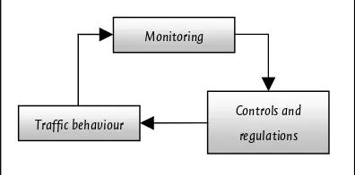
Comprehensive policies are required to cope with the growth of mobility. Transport planning and traffic management are necessary to support policy development and evaluation. Traffic management particularly focuses on the interaction between travel supply and demand. Behavioural information of the traffic is monitored by the traffic manager who regulates and controls the traffic. This is like a ‘two-way interaction game’ (Bovy & Stern, 1990).

Traffic behaviour

Controls and regulations Monitoring

(12)

Page 2

To improve policy making and policy evaluation transport models are used. These models can be used to determine the effects of traffic measures. Offline models are used to forecast traffic demand and flow patterns based on zonal data and empirical data like traffic counts. Online models use real-time data. For this research offline models are considered.

A common modelling approach consists of the four steps of trip generation, trip distribution, modal split and traffic assignment. For the traffic manager, especially the assignment stage is interesting, because it supplies in estimation of the effects of (dynamic) traffic measures before they are applied in real-life. For a comprehensive overview of the traffic assignment problem and related issues, see Patriksson (1994).

1.2 Research

motive

Dynamic Traffic Assignment (DTA) models can be used to estimate the network load over time based on dynamic travel demand. Since the research of Merchant and Nemhauser in the late 1970s - which may be considered as the basis for all dynamic traffic assignment models - DTA modelling has evolved many times (Bliemer, 2001). However, it is still considered as relatively undeveloped (Peeta & Ziliaskopoulos, 2001).

DTA models contain two interdependent components: route choice and dynamic network loading. Route choice models determine the behaviour of flows in the network. Dynamic network loading (DNL) describes the flow propagation through the network. A distinction can be made for two types of DTA models.

The first type uses one comprehensive framework in which route enumeration and flow propagation is performed merely analytical. Relatively easy link performance functions are used, e.g. linear link exit functions (Bliemer, 2001). This simplicity enables the model to use advanced existing mathematical techniques to solve the DTA problem. The realism of traffic propagation thereby is of secondary importance (Szeto, 2003). The benefit of this approach is that existence and uniqueness of a solution can be proven (Yperman, 2007).

(13)

Page 3

A problem with many of the existing DTA models is that they often focus on either route choice or dynamic network loading. Especially the models with advanced DNL (sub)models lack the implementation of route choice. However, DNL models recently received more attention, merely because of their improved ability of capturing flow dynamics (Bliemer, 2001).

The presence of good DNL models raises the question whether such models could be extended to full DTA models. This requires solving the route choice problem and implementing the interaction between route choice and dynamic network loading. The literature does give theoretical information on the first subject, but practical information is not widely available. Further the interaction between route choice and dynamic network loading is a subject that deserves more attention.

1.3

Objective and research questions

The objective of this study is to contribute to transport modelling by presenting a framework that extends existing DNL models with route choice.

“The aim of the study is to develop a route choice model as an extension for current macroscopic DNL models, taking into account the interdependence of route choice and network loading.”

In order to support the accomplishment of the objective two research questions are formulated.

1. What are the specifications of a route choice model as part of a dynamic traffic assignment model?

2. How can the iterative characteristic between dynamic network loading and route choice be realised?

1.4 Research

context

(14)

Page 4

1.5

Scope

of

study

Before exploring the contents of this report, it is important to note what is part of the research presented and what is not.

Type of assignment

The study is focussed on macroscopic dynamic traffic assignment. Occasionally there are some references to static assignment techniques.

Level of detail

The study is used for the development of a route choice model to be used in medium to large scale networks, comprising up to 4000 zones and 200.000 links. When defining the route choice model and the interaction between route choice and network loading, this order of magnitude is considered, which means the level of detail is relatively limited.

Departure time modelling

Departure time modelling is not under investigation in this research.

Modes and purposes

Only one travel network is considered: the motorway network. The number of modes and purposes is limited to comply with the desired level of detail: The model abstracts to only 1 mode and different types of network users (and so purposes) are represented by user classes.

Propagation modelling

Although propagation modelling is an important component in DTA modelling, it is not under investigation in this report.

Data use and calibration

(15)

Page 5

1.6 Report

outline

This research is structured as follows. Chapter 2 gives an introduction to traffic assignment; first explaining static assignment and then presenting the reasons for dynamic traffic assignment.

In chapter 3 a conceptual framework is presented that contains all elements that are elaborated in the chapters 4-7. First chapter 4 discusses route choice and routesets from a theoretical perspective.

In chapter 5 route choice is presented as a discrete choice problem. Random utility maximisation theory is used to express route choice models from both the Logit and Probit family. A central focus is on special route choice models developed in recent years. These models are analysed in chapter 6. A selection from a real network is used to simulate model performance and see how well the models perform.

Chapter 7 focuses on the interaction between route choice and dynamic network loading. Solution algorithms are investigated and presented mathematically. Chapter 8 will test a new algorithm using a case study.

(16)

Page 6

2 Traffic

Assignment

overview

This chapter focuses on dynamic traffic assignment from both a theoretical and practical perspective.

In paragraph 2.1 traffic assignment will be introduced in general, followed by discovering different types of traffic assignment in paragraph 2.2. Paragraphs 2.3 and 2.4 focus on static and dynamic assignment respectively. The chapter ends with paragraph 2.5 on the MetaNET/MaDAM model.

2.1 Introduction

Traffic assignment is the fourth stage in the classic four-step transport planning approach. As described by Ortúzar and Willumsen (2001), the assignment model determines an optimal trade-off between supply and demand, based on some given decision rules. The decision rules include the route choice behaviour of the travellers in the network. In practice, it means all trips are assigned to the network resulting in a traffic flow pattern.

Compared with the network’s infrastructure, the resulting flow pattern gives information about the performance of the network. For the traffic manager this is necessary information when determining effective management techniques.

2.2

Types of traffic assignment

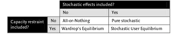
Assignment models are subject to the assumed traveller behaviour and network performance. If the model takes into account delays due to travel demand, the model is capacity restrained. Travellers route choice depends on the costs of the available routes. If the travellers are assumed to have perfect knowledge of the network conditions, a full equilibrium is simulated. If perception differences are simulated, the assignment model yields a stochastic flow pattern.

Stochastic effects included?

No Yes

No All-or-Nothing Pure stochastic Capacity restraint

included? _Yes _{Wardrop's Equilibrium} _{Stochastic User Equilibrium} Figure 2.1 Types of traffic assignment

(17)

Page 7

2.3

Static traffic assignment

2.3.1 Static equilibrium definitions

Based on the classification scheme in figure 2.1 the following static equilibria are distinguished.

Wardrop's First Principle (User optimum)

The first principle states that under equilibrium conditions, no individual trip maker can reduce his path cost by switching routes. This means that all used routes between an origin and destination have equal impedances and all declined routes have larger impedances. This principle is also known as the User Optimum.

Wardrop's Second Principle (System optimum)

Wardrop’s second principle, also known as the System Optimum, defines a state in which the network total travel cost is minimised. This means no single traveller can change routes to reduce his costs without thereby increasing the travel costs of other travellers (Wardrop, 1952).

Stochastic User Equilibrium

Under equilibrium conditions, no individual trip maker believes he can reduce his path cost by switching routes.

2.3.2 Static assignment algorithms

Although other algorithms are possible (and gaining attention), widely used static assignment algorithms are based on repeated shortest path searches and dynamic network loading. The techniques differ in the way they assign the traffic to the network: incrementally, by convex combination or by using a line-searching technique (Frank-Wolfe algorithm). If a solution flow pattern exists, such methods will converge to this solution1.

For a comprehensive exploration of (mathematical) assignment algorithms, see Sheffi (1985) and Patriksson (1994).

2.3.3 Uniqueness of solution

If an equilibrium flow pattern exists and is unique, this solution is by definition only unique in terms of link flows. Multiple route flow patterns may result in the same link flow pattern and therefore there is not by definition a unique route flow pattern that results in a equilibrium traffic situation.

_____________________________

1

(18)

Page 8

2.3.4 Drawbacks of static assignment

In the static case travel demand for a certain period is known (for instance a morning peak period). One single OD-matrix contains the trips, which are all assumed to start and end within this period.

Some remarks must be made on static assignment. First, recalling from the previous paragraph an equilibrium solution – if one exists – exists only in terms of link flows and not on route level per se (although it is theoretically possible in some small networks). Secondly, for longer trips (most of) the static assignment models do not take into account that trips might not reach their destination within the modelled time period. This aspect has recently received attention in a paper by Clark et al. (2007). The largest drawback of static assignment models is that they do not take into account the traffic flow through the network over time.

2.4

Dynamic traffic assignment

DTA models overcome the limitations of static assignment models by using a dynamic network loading model. Such a model uses continuous or discretised2 time to model traffic flow through the network. Compared to static assignment models, congestion effects are simulated far more realistic.

Dynamic Network Loading model (propagation model)

In dynamic assignment modelling, a propagation defines the interaction between traffic on the network, like headway interaction, speed-density relations and stop- and go actions. Several propagation models have been developed over time, varying from car-following theory to kinematic wave and gas flow theory.

2.4.1 Application of assignment models

In the past static assignment techniques have been used on a large scale. During the last decade a shift toward more use of dynamic models can be seen. There are two major causes for this trend. First, the demand from the market has changed. For a long period there was practically no need for dynamic assignment models, since static models gave (and still give) robust results for the purpose of transport planning. Over time the market (consultants and their clients) also wanted insight in travel times (and delays) and queue building. This required a model that took time dynamics into account. Secondly, the computational power needed for DTA models is huge and until the late 1990s required special computers. With the increasing possibilities of regular computer workstations the dynamic traffic assignment is gaining importance rapidly (Peeta & Ziliaskopoulos, 2001).

_____________________________

2

(19)

Page 9

2.5 The

MetaNET/MaDAM

model

As described in paragraph 1.4 the study presented here is carried out at Omnitrans International (OTI). The DTA model MaDAM, based on the DNL model METANET, is developed at OTI. Because the findings of the presented study might be used in the process of redeveloping MaDAM, it is important to briefly describe the current MaDAM model.

2.5.1 METANET

The basis for MaDAM lies in the METANET model, developed by Messmer and Papageorgiou in the 1990’s. In METANET time and space are discretised. The network is represented by a directed graph, where links are singly directed and the geometrics for a link are assumed homogeneous. Nodes between the links are used as diverge or converge points or at locations in the network where the motorway characteristics change (e.g. number of lanes). A large restriction however is that only nodes of degrees 2 and 3 are possible, which makes it inefficient to model realistic networks (Van Berkum, 2007).

For each link a fundamental diagram is assumed, based on the link parameters free flow speed, speed at capacity, jam density and saturated flow. To propagate traffic, the METANET model divides the links into segments of equal length. All flow variables are calculated for each segment, using the fundamental diagram and using traffic conservation equations to be realistic with the conditions on the segments upstream and downstream.

Route choice behaviour is presented by defining splitting rates for cross- and diverge nodes (nodes with multiple exit links). Both the travel demand and the splitting rates (turn fractions) may change over time, as specified by the user.

2.5.2 MaDAM

There are three major differences between MaDAM and METANET, which makes them two different models. The first major improvement is the ability to use nodes of higher degrees in MaDAM. This makes it possible to model full intersections (i.e. with 4 entering and 4 exiting links).

The second major change is the use of a different fundamental diagram compared to METANET. According to the developers of MaDAM the original fundamental diagram from Metanet gives unrealistic results when volume approaches capacity the speed drop is too large, while they believe in such situations still relatively high speeds can be reached. Therefore, the Van Aerde fundamental diagram is used, which addresses supplies in this concern.

(20)

Page 10

3 Conceptual

framework

The previous chapter has introduced the concept of dynamic traffic assignment. This chapter will present a conceptual framework and gives a short introduction to the chapters 4, 5, 6 and 7.

The DTA framework has to be consistent with existing Dynamic Network Loading models, but add (or replace existing) route choice models. The framework contains a route choice module that is fully flexible with – and operates independently of the used DNL model for propagation.

Paragraph 3.1 starts with defining the variables used in the framework, followed by a short outline of the framework in paragraph 3.2. The model constraints are investigated in paragraph 3.3. The concepts of route choice and DNL-Route choice interaction are discussed in paragraphs 3.4 and 3.5.

3.1 Variables

The mathematical formulations of the framework use index characters to define to which elements data is related. The following indices are used.

3.1.1 Location variables

Origin (o)

Zone in the network from where traffic departs.

Destination (d)

Zone in the network where a trip ends.

Route (r)

Series of links from an origin to a destination zone.

Position (x)

A position along a route is denoted by

x

. This location is route, departure interval and time dependent.

3.1.2 Time variables

General time (T, t)

The framework uses multiple time dimensions. The total (continuous) modelling period is denoted by

T

. Index denotes a moment within this period. This index is continuous or discrete, depending on the used dynamic network loading model.

(21)

Page 11

Route choice interval (k)

The total time is divided into several time windows. In each time window the route choice behaviour is equal i.e. all travellers are assumed homogeneous. The length of such a time interval is quite arbitrary. If many small time windows are used, the traveller behaviour tends toward a microscopic model (since only small fractions of vehicles are considered equally behaviouring). is used as additional index for .

k

t

Forecasting horizon (λ)

A forecasting horizon might be used (more info in paragraph 7.5), where

λ

is used as additional index for

t

.

Time aggregation (γ)

Data is aggregated in equal time intervals, where the size of an interval is defined by the modeller.

Time-location example

rod t_k

x

δ defines the point on route

r

from origin

o

to destination

d

, departing in route choice interval

k

,

δ

time units after departure. If

δ

=

∞

this means the end of the route.

3.1.3 Network variables

Link (a)

Element of the network at which time-dependent traffic conditions are stored.

3.1.4 Traveller variables

Individual (n)

For theoretical modelling an individual traveller

n

is considered.

User class (u)

(22)

Page 12

3.2 Framework

outline

The conceptual framework is depicted in figure A.1 on the page 67 (this figure can be folded out for viewing while reading). Based on previous steps in the transport model, travel demand is assumed to exist for each time period and user class. Travel cost functions are used to determine the routeset (generate and filter). The main part of the DTA model framework consists of loops in which route choice and dynamic network loading are iteratively optimised to derive the flow pattern meeting a set of constraints.

Multiple user classes

Dynamic traffic assignment models using a discrete choice model for stochastic route choice allow some variation among travellers, but the traveller population is still considered homogeneous. Bliemer (2001) and Rosa & Maher (1999) suggest to extend DTA models with the inclusion of multiple user classes to represent heterogeneous traveller characteristics and thereby increase model applicability and make them more realistic.

In the presented framework multiple user classes are supported for all model elements except the dynamic network loading model. Depending on the DNL model used, user information might not be used during traffic propagation. The framework however is flexible and is still able to evaluate route choice for each user class after propagating.

3.3 Constraints

The dynamic network loading model used for reference in this study employs a route structure in which route choice is allowed only in the departure (origin) zone. Once traffic is assigned to a route, the flow on this route can not be (partly) reassigned to another route.

Pipe concept

(23)

Page 13

Flow in the pipe is dependent on the conditions at the links in the top layer, the actual network. Density is equal for all pipes under the same link, but speed and flow may differ since alternate fundamental diagrams may be used for each layer. For instance heavy freight trucks will have a lower maximum speed on the highway than regular cars. For each time step in the dynamic network loading process, the density on all links is updated based on the in- and outflow (for all pipes).

3.4

Route choice concept

The framework is developed for application on large scale networks. Path searching while running the model will dramatically reduce model performance and is considered unnecessary if an adequate routeset is known beforehand. Therefore the routesets are to be derived before running the actual model. Discrete choice modelling is used to calculate probabilities for the routes in the routesets.

3.5 Interaction

concept

(24)

Page 14

4

Theory on route choice and routesets

This chapter describes the basic theories on routes. This includes both theoretical requirements on the knowledge of route choice as traveller behaviour and a global overview of routeset generation and filtering.

Paragraph 4.1 starts with exploring the characteristics of route choice. This is followed by a brief investigation of route choice factors in paragraph 4.2. Paragraph 4.3 is on theory of routeset generation, 4.4 on randomisation techniques and 4.5 on routeset filtering.

4.1

Route choice basics

Bovy and Stern (1990) have investigated wayfinding and factors of route choice thoroughly. One of the basic fundamentals they state is that route choice is individual behaviour. For a macroscopic model we therefore assume route choice of a group is the result of many individual choices. Such an approach requires we first understand individual route choice behaviour. The next step is to determine how the choice of many individuals can be represented by choices made by a population.

4.1.1 Types of route choice

Based on observations, three types of route choice are defined (Bovy & Stern, 1990):

• Simultaneous choice

• Sequential choice

• Hierarchical choice

Before explaining what these types are, a definition is presented.

Decision point

A decision point is a node in a network where two routes of the set of alternatives for an origin and destination combinations split. The first decision point is the trip origin.

Simultaneous choice

The traveller makes a choice for a route before making the trip. The choice set contains routes between the origin and destination of the trip.

Sequential choice

(25)

Page 15

Hierarchical choice

The hierarchical choice is similar to the sequential choice except for the probabilities to choose an alternative. In the case of sequential decision making the choice of the next subroute is independent of previous choices, while in hierarchical decision making this probability is dependent.

In practice all three types of route choice occur (Jansen & Den Adel, 1987; Stern & Leiser, 1988; Benshoof, 1970; all in Bovy & Stern, 1990). However, even in simultaneous route choice it is likely that travellers can be forced to change routes because the route they did choose is no longer available, for instance because an incident has blocked a tunnel. This is referred to as adaptive route choice.

Adaptive route choice

When the traveller decides to change his (initial) route choice while travelling, based on changing circumstances he encounters, this is called adaptive route choice.

The introduction of vehicle navigation systems have lead to an increase in adaptive route choice in recent years. Especially devices with real-time traffic information are capable of giving optimal routes from the current position of the traveller to the trip destination.

4.2

Route choice factors

As pointed out before, each traveller is a decision maker that makes an individual choice. The choice for a route is made based on the evaluation of the alternatives the individual faces. These alternatives form the routeset.

Routeset

A routeset Sn is a set of alternative routes as observed by individual decision maker n.

(26)

Page 16

Examples

An ambulance driver will choose the alternative with the smallest and most reliable travel time and the least amount of speed bumps. A truck driver might be forced to use a specific route because his load contains specific materials that are only allowed on designated roads. And someone who travels to his work daily will probably always take the same route, independent of route characteristics, unless the route quality changes significantly.

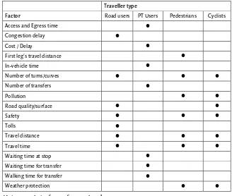
Previous research has shown that route-specific attributes are the most important (Bovy & Stern, 1990, pp. 65-68; Fiorenzo-Catalano, 2007, pp. 110-112). An overview of route-specific choice factors for different traveller types as given by Fiorenzo-Catalano (2007) is summarized in table 1.1. Of course this list is incomplete. For more information see Bovy and Stern (1990, table 3.3, p. 68).

Traveller type

Factor Road users PT Users Pedestrians Cyclists

Access and Egress time z

Congestion delay z

Cost / Delay z

First leg's travel distance z

In-vehicle time z

Number of turns/curves z z z

Number of transfers z

Pollution z z

Road quality/surface z z

Safety z z z

Tolls z

Travel distance z z z

Travel time z z z

Waiting time at stop z

Waiting time for transfer z

Walking time for transfer z

Weather protection z z

Table 4.1 Main route choice factors for travel modes

(adapted from Fiorenzo-Catalano, 2007, p. 111)

4.3

Routeset generation and filtering

(27)

Page 17

It is important to understand that the route choice process is implicit and travellers can only to some extent explain their choice. The process of routeset generation is even more implicit. This means that we have to use model techniques to define the route choice set.

Fiorenzo-Catalano (2007) has develop a framework for the routeset generation process, including 4 basic steps in routeset generation:

• Step 1: Search a best route according to certain conditions;

• Step 2: Evaluate the route to a set of route criteria;

• Step 3: Select or reject the generated route;

• Step 4: Evaluate the resulting route set according to a set of criteria.

4.3.1 Types of routeset generation

In general there are three types of route generation:

• Single objective function search

• Multi-objective function search (Label search)

• Derive from capacityconstrained traffic assignment

The first and second approach use an objective function.

Objective function

The objective function is a function that represents the observed quality of a route by a decision maker. The function includes the attributes the traveller considers important (such as those described in table 4.1). The objective can be to minimise the function (e.g. the route length) or to maximise the function (e.g. route utility).

The objective function is not limited to continuous values like link length and travel time, but can also be based on discrete values. For instance, a path search can be done to find the path with the smallest number of traffic lights.

4.3.2 Single objective function search

This generation type is based on a single, fixed objective function. The search for the shortest path in a network is an example of this type of routeset generation.

4.3.3 Label search

(28)

Page 18

Example

An example of label search could be making a routeset with the shortest path, the fastest route, the route with the least number of speed bumps or the route as suggested by traffic signs.

Techniques for multiple routes from objective function(s)

For both techniques based on an objective function multiple routes for each objective function can be found by applying Monte Carlo simulation, where in each draw the attribute values – and thereby the objective function – take different values for each link. This results in other ‘shortest paths’. An other technique is to eliminate one or more links in the path search process and thereby derive alternative ‘shortest paths’ which are added to the routeset.

For more information on techniques for the generation of multiple routes from objective function(s) see Fiorenzo-Catalano (2007), page 161 and further.

Previous applications

Ben-Akiva et al. (1984) have proposed a labelling method using a large number of optimality criteria based on surveyed choice motivations. An optimal path is found for each of the criteria: shortest route, quickest route, best signposted route, scenic route, etc. Bekhor & Toledo (2005) state that six labels could cover about 90% of all travelled routes. Others suggest that approximately between 60 and 80 percent of the travelled routes can be identified (Ortúzar & Willumsen, 2001, pp. 328).

4.3.4 Derive routeset from capacity constraint traffic assignment

With capacity constrained assignment multiple path searches are done with the same objective function. The value of the link attributes are influenced each iteration by the assigned traffic rather than randomised. In the end, the routeset contains paths found as a shortest path in all iterations. Using this method, the routeset is dependent on the used assignment algorithm and its parameters (e.g. the fractions in incremental assignment or the number of iterations when using volume averaging techniques).

Example

(29)

Page 19

4.3.5 Shortest path search

For the first and second type of routeset generation a shortest path search is used. This paragraph explains briefly what path search is and the elements of the basic algorithm.

Shortest path search

Shortest path searching is the process of finding the sequence of links in a weighted graph with minimal impedance.

Path search algorithm

There is a wide variety of shortest path algorithms available. However, the basis of all these methods is the tree-building algorithm of Dijkstra (1959). This efficient node-by-node algorithm is very effective. For transport planning however, the presence of forbidden turn movements on intersections can not be modelled by the algorithm. A link-by-link algorithm has to be used.

4.4

Theory on randomisation

To find routes that are suboptimal either the shortest path must be ignored or have a larger impedance or a suboptimal path has to be have a lower impedance. A known technique for the first approach is used in the Marple traffic model, where repeated shortest path searches are performed and the impedances of the links of the found are multiplied by a factor. A drawback of this approach is that new found paths are unlikely to (partially) overlap with already found paths and therefore might lead to a unrealistic routeset.

Using randomisation techniques routesets can be generated that do not exhibit the drawback described above. Further they allow suboptimal paths to be found as optimal paths.

Randomising the link attributes is based on the fact that the link attributes are perceived differently among travellers. Examples of such attributes are travel time and travel distance. In the routeset generation process this behaviour is simulated.

General outline of Monte Carlo simulation

(30)

Page 20

Link attribute values are randomised using random number generators on a computer. Scaling problems might occur when absolute random numbers are generated: there is a large difference between the random outcome of 2 time units when travel time is measured in minutes or in hours. Relative random numbers do not exhibit this problem.

Distribution random function

The literature is not specific on what set of parameters and what distribution is to be chosen for optimal routeset generation. The choice for a set of parameters is quite arbitrary, but since routeset generation is mostly followed by a filtering process, the final routeset can be derived in many ways.

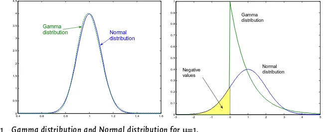
In this research the randomisation is assumed to be based on distribution of the link attributes, where each attribute might have a specific distribution. For many uncorrelated attributes the central limit theorem states that the link impedance is normally distributed.

One problem arises when using the Normal distribution. In the process of path searching it is required that no cyclic paths are found, and therefore all link weights should have the same sign. Using a Normal distribution with mean 1 (relative factor for link impedance) can however result in negative values. From the theory of attribute perception this is unlikely: a traveller might perceive an attribute value in a more positive way, but it is not likely to perceive this value having another sign.

0.4 0.6 0.8 1 1.2 1.4 1.6

Figure 4.1 Gamma distribution and Normal distribution for µ=1. (Left figure σ2

= 0.1, Right figure σ2 = 1)

(31)

Page 21

Accelerated approach

The Accelerated Monte Carlo approach uses an initial low variance. When after some draws no new routes are found, the variance increases, leading to larger changes in the link impedances. The idea is that then routes are found further away from the shortest path.

4.5 Routeset

filtering

Apart from the question of how routesets are generated, it is important to identify the specifications for adequate routes and routesets. Fiorenzo-Catalano (2007) presents a framework containing definitions of Dial (1971) and Hoogendoorn-Lanser (2005). This framework consists of requirements for single routes, comparing between routes and the total routeset and will be described briefly3.

Requirements for single routes

• Reasonable routes are a-cyclic. All links have positive impedance values (Acyclic criterion).

• A reasonable route does not exhibit a detour from the shortest possible connection in terms of one or more measures such as distance or time between origin and destination larger than a maximum threshold α. (Detour criterion)

• A reasonable route is constituted by a systematic sequence of functional link levels, avoiding route parts going from higher to lower level links and back. (Hierarchical quality criterion)

Requirements for comparing alternative routes

• The mutual overlap between two alternative routes is less than ∆ percent with respect to the shorter one of the two routes (Overlap criterion)

• Any two routes of the choice set should be comparable in travel (dis)utility within a given threshold of θ percent with respect to the shorter one of the two routes (Comparability criterion)

• The non-common parts of two partly overlapping routes should have a maximum detour not larger than a given maximum percentage ω_max of the minimum two parts (Detour-max criterion)

• The non-common parts of two partly overlapping routes should have a minimum detour not smaller than a given minimum percentage ωmin of the

minimum two parts (Detour-min criterion)

_____________________________

3

(32)

Page 22

Requirements for total route set

• All reasonable routes that are likely to be used are part of the routeset (Reasonable criterion)

• The size of the routeset is limited to a predefined number of S routes (Choice set size criterion)

(33)

Page 23

5

Route choice as discrete choice problem

In this chapter the route choice problem is described as a discrete choice problem. Several choice models are presented as possible methods to deal with the route choice problem. The models are described from the underlying theory of random utility maximisation. The descriptions are used to make a choice in the next chapter on what route choice model is preferred for application.

This chapter starts with an introduction in paragraph 5.1. Paragraph 5.2 gives an introduction to random utility maximisation theory. Basic discrete choice models are presented in 5.3. A problem arising when using these models is mentioned in 5.4 followed by exploring alternative discrete choice model formulations in paragraph 5.5. Finally, paragraph 5.6 presents a simulation technique.

5.1 Introduction

In this chapter the following conditions are considered. A predefined routeset is used, containing a limited set of alternatives for an OD-pair. The modeller can specify utility functions which may include both fixed characteristics of the network (e.g. speed bumps) and measures of dynamic network performance. The choice model is supposed to result in the probabilities of a population of travellers choosing the specified route from the routeset.

5.2

Random Utility Maximisation theory

Route choice can be seen as a discrete choice problem. Random Utility Maximisation theory assumes that each traveller will try to maximise his utility when making this choice.

n

Assume the routeset

S

_n

=

{

R

₁

,

R

₂

,...,

R

_j

,...,

R

_J

}

consisting of J alternatives. Each alternative known by decision maker all have a personal utility , so

the decision maker will choose alternative for which

n

U

nj

(34)

Page 24

Although it is theoretically possible that the researcher can define the exact utility, it is assumed that in general the representative utility approximates, but not equals the actual utility:

V

_nj

≠

U

_nj. Therefore

U

_nj

=

V

_nj

+

ε

_nj, where

nj

ε

captures the attributes that influence the utility of the decision maker, but are unknown to the researcher (Train, 2002). Bierlaire (2005) defines

ε

_njas the capture of the maximum of many unobservable attributes and specification errors. Since

{

ε

_n₁

K

ε

_nJ

}

are unknown, the set is assumed to be randomly distributed.

The probability a decision maker chooses alternative can be rewritten in terms of the representative utility:

i

Given the cumulative distribution of

ε

_n, the probability becomes

)

The probability is a multidimensional integral over the distribution of

ε

_n. The definition of

f

( )

ε

_n defines the choice model. Only for certain specifications of

( )

n

f

ε

a closed form solution of the multidimensional integral exists.

5.3

The Probit and Logit model families

In general, two families of choice models can be considered. Within the families variants may exist. The families are distinct since they have different base assumptions on the distribution of the unobserved portion of the utility function.

5.3.1 Multinomial Logit

The Logit model is derived under the assumption that

ε

_niis distributed IID Extreme Value Type 1 for all :

i

(35)

Page 25

Multinomial Logit

(5.4)

The probability function has a very convenient form, which makes it a popular model and easy to apply. However, the MNL model exhibits the IID-property: the unobserved factors are considered independent and identically distributed. This results in equal variances for all alternatives (Train, 2002). For application in route choice situations, this means the model does not take overlap and different variances among alternative routes into account.

∑

5.3.2 Multinomial Probit

The Probit model is derived under the assumption that

ε

_niis multivariate normally distributed with a vector of means

0

and a variance-covariance matrix. The probability for an alternative can be written in RUM terms as

J

×

Multinomial Probit

(5.5)

where

φ

( )

ε

_n is the joint normal density with zero mean and the defined variance-covariance matrix. No closed form solution exists for the Probit Model. The probabilities are evaluated numerically through simulation (an algorithm to perform such a simulation is described in paragraph 4.6).

µ

5.4

The overlap problem

In route choice modelling overlap between routes defines a correlation between the error terms and thereby influences the choice probabilities.

Overlap

(36)

Page 26

An example of the overlap problem is presented in (Sheffi, 1985, p. 294). For effective route choice modelling, overlap should explicitly be taken into account in order to prevent wrong outcomes (Frejinger & Bierlaire, 2007). In the Probit model the variance-covariance matrix is explicitly defined. But since this method requires simulation it is far slower in performance than the Multinomial Logit model.

5.5

Alternative Logit formulations

During the last two decades alternative Logit formulations have been developed that capture the correlation among alternatives. A classification can be made on how these models take correlation into account.

5.5.1 Common links define nest structure

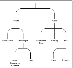
The MNL model does not contain levels. An extension is given by the Nested Logit model, where alternatives are placed in nests. Each nest contains correlated alternatives. Alternatives among different nests are uncorrelated. The bottom level nest is equal to a standard MNL model. Theoretically it is possible to define a model with a large number of levels (where each nest might contain subnests). See figure 4.1 for an example of a nested model for mode choice.

Figure 5.1 Example of nesting structure in mode choice (From: Ramming, 2002, p. 37)

Cross-Nested Logit (CNL)

In the Cross-Nested Logit, the Nested Logit model is extended by a correlation parameter which makes it possible for an alternative to belong to several nests with different degrees. The degree of correlation is defined by a parameter

)

1

0

(

≤

_mi

≤

mi

α

. This parameter was defined by Vovsha and Bekhor (1998)

(37)

Page 27

information see (Ramming, 2002, pp. 49-52). One important limitation pointed out by Fiorenzo-Catalano is that for realistic routes containing many links and larger routesets the nesting structure would be extra-ordinarily complex (2007, p. 126).

The probability is defined by

(

)

(

)

General Nested Logit (GNL)

The General Nested Logit is an extended formulation of the CNL model. GNL allows an extra dissimilarity parameter between nests. In practice this would mean that links in different nests would contribute on different scales to the representative utility, which contradicts the concept of representative utility. This concept requires all links to be comparable, i.e. to have equal scales. According to Fiorenzo-Catalano (2007, p. 126) this makes GNL unusable for route choice modelling, although there might be some exceptional cases.

Paired Combinatorial Logit (PCL)

The Paired Combinatorial Logit uses a correlation parameter for each combina-tion of routes (e.g. i and j) in the routeset. This correlacombina-tion parameter is given by

1

(

1

−

η

kh is a measure of the correlation between the alternative routes.

Because only each combination of alternatives has to be investigated, the structure of a PCL is less complex than the nested structure of CNL/GNL and thereby provide a computationally tractable mechanism for the route choice problem (Fiorenzo-Catalano, 2007, p. 126).

(38)

Page 28

with scale parameter

µ

and

S

defining the size of the choice set.

5.5.2 Common links define disutility component

The second type of alternative Logit formulations use a disutility component for accounting the overlap. The general idea behind this approach is that when making a choice between two partially overlapping routes, only the utility for the non-overlapping section is competitive and influences the decision. This approach is also known as penalising.

C-Logit (CL)

The C-Logit model penalises the alternative’s utility function by a Commonality Factor (CF). This factor is defined as

1 where

γ

₀ and

γ

₁ are positive parameters and have to be estimated

(Fiorenzo-Catalano, 2007, p. 127). The difference in approach compared to PCL is that the factor is measured compared to all other alternatives in the set, while PCL makes a comparison for each combination of two alternatives. After application, testing and calibration, Ramming concludes that C-Logit does not give useful results for his case study in Boston for which route choice data was available (Ramming, 2002, p. 190).

Path Size Logit (PSL)

The Path Size Logit model uses a penalty for the Utility function, similar to the C-Logit model. The model is based on the Path Size-parameter PS, which is defined as (Generalised Path Size Logit)

(39)

Page 29

where

a

∈

R

_irepresents all links in route , is the length of link a, represents the length of route and

i

l

a

d

i

δ

_aj is a binary value that is equal to 1 if link

a

is present in alternative

j

and

0

otherwise. The parameter

γ

needs to be estimated (Hoogendoorn-Lanser et al., 2004).

The probability is defined by

( )

The Path Size Logit formulation is argued to sometimes give counterintuitive results (Bierlaire & Frejinger, 2005).

5.6

Probit simulation technique

5.6.1 Introduction

Although the Probit model can not be applied directly, a simulation technique can be used to derive choice probabilities. The simulation algorithm is described by Sheffi (1985). The basic principle is to randomise link cost values and thereby randomise the route utilities taking the overlap directly into account. When this is done for a large number of draws a multi-dimensional integration is simulated. Route probabilities are calculated from the percentage of draws a route is simulated as ‘shortest path’.

5.6.2 Algorithm

For each OD-pair, consider a routeset

S

OD

=

{

R

₁

,

R

₂

,...,

R

_i

,...,

R

_J

}

. The links present in the routeset form the set

L

=

{

l

₁

,

l

₂

,...,

l

_a

,...,

l

_A

}

. The objective function uses travel cost and the aim is to minimise the function value.

X

is initialised as a zero-vector with J elements.

In each draw the link costs (or utilities) are randomised by applying

( ) (

) ( )

C

L

C

*

l

_a

=

1

+

ζ

_a

⋅

0

l

_a

∀

l

_a

∈

(5.12)

Because we are using the Probit model, we assume the random term

ζ

_ato be

(

)

a

(40)

Page 30

After randomising the link travel cost, the link costs are summed over the links in a route to derive the random route travel cost, C*:

( )

∑

( )

Now route costs are known for all routes in the routeset (for this draw). One of

those routes has the lowest cost. This increases the number of draws for which the alternative is preferred.

( )

After all draws, the probabilities for each alternative are given by

(41)

Page 31

6

Route choice model analysis

The previous chapters have given an introduction to available route choice models. The purpose of this chapter is to analyse which route choice model is best to use for large scale application and therefore should be implemented in the framework. Thereto model performance is analysed using a case study.

This chapter starts with looking at relevant previous research in paragraph 6.1. In paragraph 6.2 the approach used for the performance analysis is presented. A case study is presented in paragraph 6.3. The analysis and test results can be found in paragraph 6.4 and discussed in paragraph 6.5. A remark on discrete choice models is made in paragraph 6.6. In paragraph 6.7 a proportionality factor is introduced, followed by a conclusion on which model is best to be used in paragraph 6.8.

6.1 Previous

research

All of the models in the previous chapter are well described (from a theoretical point of view) in scientific literature. The amount of publications on practical application of the models by others than those who defined them is however very low. Only two publications are worth mentioning. Ramming (2002) gives a thorough investigation of the models. He used the Path Size Logit model to calibrate data from a case study in Boston. Information on the quality of other models is not described.

More recent Bliemer and Bovy presented a paper in which they compared various Logit models using the Probit model. Their focus was on the prediction quality of the route choice models in dependence of the size and composition of pre-defined routesets (Bliemer & Bovy, 2008). They used a Probit simulation technique to determine fictive route choice probabilities and calibrated the Logit models against those. Then they changed the size of the choice set (adding or subtracting routes) to see how well the calibrated models approached the new calculated Probit simulation route choice probabilities. They found that none of the investigated models (MNL, C-Logit, CNL, PSL, PSCL and PCL) are robust and all models lead to incorrect probabilities after changing the size of the choice set. In their experiment Bliemer and Bovy used a simple 1 origin, 1 destination network containing 12 links.

6.2 Approach

(42)

Page 32

sizes. Does this mean the route choice models are all useless or can we determine for what conditions the models give better or worse results?

This chapter investigates model performance of 5 Logit-based route choice models (MNL, CNL, PCL, PSL and C-Logit). The approach used is quite similar to the one used by Bliemer and Bovy. The simulation technique described in paragraph 5.6 is performed with a sufficiently large number of draws to derive route choice probabilities. The Logit-based models are then calibrated (at network level) against those probabilities. At level of routesets (per OD-pair) the model performance is then analysed against properties of the routeset.

6.2.1 Number of draws needed

To make realistic comparison between model performance, the number of draws used in the Probit simulation has to be large enough. Otherwise the stochastic spread in the probabilities from the simulation is too large. Therefore, the number of draws needed in the Probit simulation technique has been investigated.

Approach

In total 1.000.000 draws have been made, split up in batches of 100 draws. For each batch the route probabilities are calculated. By averaging over batches the number of draws increases and the probabilities converge to the average of all draws. For example, for the sixth batch the probabilities for the first six batches are averaged (assumed as 1 batch of 600 draws). The difference between the simulated probability for this collection of batches and the overall average probability is a measure for the robustness.

Mathematical formulation

Let denote the route choice probability for route

i

from a certain routeset as simulated in batch

b

. The ‘correct’ probability is assumed to be the average of 1.000.000 draws, e.g. the average of the probabilities of all batches:

b

The average pr ability of a collection of batches is given by

(43)

Page 33

The relative difference between the probability in a collection of batches and the overall average is given by

i

This indicator for robustness can be calculated for multiple routes in a set and for multiple routesets, resulting in an indicator for robustness of the Probit simulation technique for varying simulation sizes.

Results

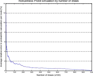
As expected the number of draws affects the robustness of the Probit simulation. A larger number of draws leads to a smaller relative error in the probability calculation. Figure 6.1 shows the relative absolute error (average over multiple routesets) from expression 6.3 for multiple simulation sizes.

0 100 200 300 400 500 600 700 800 900 1000

Robustness Probit simulation by number of draws

A

Figure 6.1 Robustness of Probit simulation

Discussion

It can be seen that up to 20,000 draws the robustness of the simulation increases significantly with the number of draws, while after 20,000 draws the increase in model performance is relatively small.

(44)

Page 34

immense. Randomising a routeset consisting of 6 routes with 1000 draws takes between 0.5 and 1.5 seconds, depending on the number of links in the routeset. To compare: calculating probabilities for a routeset using a Logit-based model takes only a few microseconds.

Based on the results shown in figure 6.1 the number of draws needed for the purpose of this research can be set to 20,000. The relative error per route is about 1%, which is assumed low enough to compare the outcome with Logit-based models.

6.2.2 Definition of model quality

Per route the absolute difference between the probabilities from the simulation and Logit model is a measure for the quality of the model. By taking the square of this difference large errors are extra penalised.

Mathematical formulation

For a routeset the probabilities for each route are denoted by where indicates the model/simulation. The performance of a model is given by

for performance quality at routeset level. For overall performance a summation is made over routesets:

(

)

For the performance tests, a large scale Dutch main road network (Bereiksbaarheidkaart) is used. This network contains over 4000 zones and over 200.000 links. For 26 zones spread over the network a routeset is created and filtered5. The zones are both larger cities and more rural residential areas, distributed all over the Netherlands. The idea behind this approach is that routes with different lengths in both urban (more detailed network) and rural areas are selected, resulting in different type of routesets (length of route, number of routes in set and different type of overlap).

_____________________________

5

(45)

Page 35

Routesets

Free flow travel time has been used for the generation of the routesets. A filter is used to reduce the sets to a maximum of 6 different routes and a maximum overlap of 60 percent. Further small detours and infeasible long detours have been filtered out. The resulting routesets contain a total of 2148 routes (average number of routes per OD pair 3.18).

Calibration

It is important to realise that no realistic route choice is simulated, but only a comparison between Probit simulation and different Logit-based models. Therefore, calibration of the Logit models is not done against empirical data, but against a arbitrary value for the only parameter in the Probit model.

The parameter for the Probit simulation is taken equal for all OD-pairs. For selections of OD-pairs, the parameters for the Logit model are calibrated. Initially all Logit models were calibrated using the same OD selection. If the validation showed unsuccessful calibration other (random) selections were generated (per Logit model), until all models resulted in the same error value or when no further enhancement of the model could be retrieved.

6.4 Results

6.4.1 Overall model performance

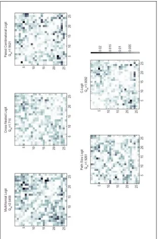
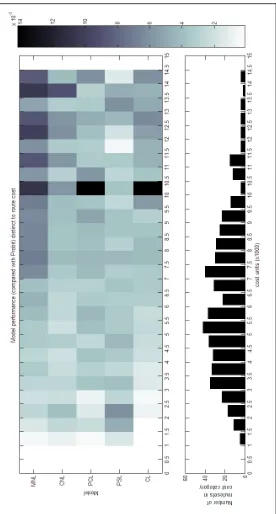
Figure 6.2 gives a first glance at model performance. Each diagram shows the sum of residuals at OD-level. The colour-scale is equal for all models, which means the darker an OD-square, the worse the model performs for the routeset of this OD-pair. is noted at the top of each diagram. Based on this first investigation one could conclude that C-Logit and Cross-Nested Logit perform better than the other route choice models. Further MNL seems to give wrong results. However, as can be seen the model performance is different among OD-pairs. This justifies a further analysis of model performance with discrimination to choice set properties.

m

(46)

Page 36

(47)

Page 37

6.4.2 Size of choice set

A distinction of model performance can be made to the characteristics of the choice set. In this paragraph the size of the choice set is considered.

Model Choice set

size _MNL _CNL _PCL _PSL _CL 2 0.2774 0.1571 0.7076 0.3179 0.1204

3 0.6698 0.4514 0.3078 0.5634 0.3099

4 0.6317 0.4114 0.3518 0.5219 0.4289

5 0.3216 0.2435 0.1870 0.2221 0.2627

6 0.6403 0.4516 0.3980 0.3009 0.4474 Total 2.5408 1.7150 1.9522 1.9261 1.5692

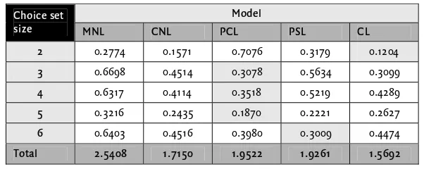
Table 6.1 Model error by choice set size

Lower values mean better performance. The best performing model for each choice set size is coloured.

Table 6.1 shows the model error (sum of squares) for subsets of the zones used in the routeset generation. Each row in the table indicates a set of OD-pairs with a different number of alternative routes. Each column indicates a Logit variant model. Lower numbers mean better performance. Because the total error is different among the models, it is difficult to compare values between columns. The values can be compared between rows to see how well the same model performs on routesets with different sizes.

Results indicate that model performance changes with choice set size. For instance, the PCL model has a large error when predicting route choice probabilities for sets with only 2 alternatives, however for sets of size 3, 4 and 5 it performs best of all. The coloured cells indicate the best performing model per row. When all errors are scaled to a total error of 1.00 per model, this colouring holds and becomes even more significant.

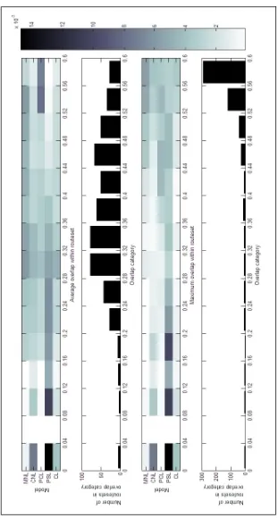
6.4.3 Amount of overlap

Model performance is analysed with both average overlap and maximum overlap. For the case study routes have been filtered with more than 60 percent overlap. For overlap ranges between 0 and 60 percent the average6 residual is calculated and plotted in figure 6.2. The figure shows that almost all of the OD-pairs with more than 1 route exhibit at least 2 routes with an overlap of more than 40 percent. The average overlap has a wider distribution among the OD-pairs. Especially this property has influen

Route choice modelling in dynamic traffic assignment