Multivariate Spatial Temporal Statistical Models for Applications in Coastal Ocean Prediction

Abstract

FOLEY, KRISTEN MADSEN. Multivariate Spatial Temporal Statistical Models for Appli-cations in Coastal Ocean Prediction. (Under the direction of Montserrat Fuentes and Lian Xie.)

Estimating the spatial and temporal variation of surface wind fields plays an important

role in modeling atmospheric and oceanic processes. This is particularly true for hurricane

forecasting, where numerical ocean models are used to predict the height of the storm surge

and the degree of coastal flooding. We use multivariate spatial-temporal statistical methods

to improve coastal storm surge prediction using disparate sources of observation data. An

Ensemble Kalman Filter is used to assimilate water elevation into a three dimension

primi-tive equations ocean model. We find that data assimilation is able to improve the estimates

for water elevation for a case study of Hurricane Charley of 2004. In addition we

investi-gate the impact of inaccuracies in the wind field inputs which are the main forcing of the

numerical model in storm surge applications. A new multivariate spatial statistical

frame-work is developed to improve the estimation of these wind inputs. A spatial linear model

of coregionalization (LMC) is used to account for the cross-dependency between the two

or-thogonal wind components. A Bayesian approach is used for estimation of the parameters

of the multivariate spatial model and a physically based wind model while accounting for

potential additive and multiplicative bias in the observed wind data. This spatial model

consistently improves parameter estimation and prediction for surface wind data for the

Hurricane Charley case study when compared to the original physical wind model. These

methods are also shown to improve storm surge estimates when used as the forcing fields

for the coastal ocean model. Finally we describe a new framework for estimating

multivari-ate nonstationary spatial-temporal processes based on an extension of the LMC model. We

compare this approach to other multivariate spatial models and describe an application to

Applications in Coastal Ocean Prediction

by

Kristen M. Foley

a dissertation submitted to the graduate faculty of

north carolina state university

in partial fulfillment of the

requirements for the degree of

doctor of philosophy

statistics

raleigh

2006

approved by:

Dr. Montserrat Fuentes (Co-Chair) Dr. Lian Xie (Co-Chair)

Dr. Jerry Davis Dr. David Dickey

Dedication

Kristen Foley was born on April 10, 1979, in Charlotte, North Carolina. In 1997 she graduated

from Northwest Cabarrus High School in Concord, N. C. She attended N. C. State University

to study engineering but was thankfully recruited to the statistics program in her freshman

year. She decided to stay in the program for her master’s degree and eventually her PhD,

which would prove to be an excellent decision. She began working with Dr. Montserrat

Fuentes during her first year on problems in environmental statistics. She collaborated on

projects with the U.S. Environmental Protection Agency to improve air quality maps and with

the NCSU Coastal Fluid Dynamics Laboratory to improve storm surge prediction. During

her time in the graduate program she worked with other students to organize a day–long

Career Fair and a new Teaching Working Group and a Research Working Group. She was

also involved in several social activities including organizing a Departmental Feud Game

Show, a canoe trip and multiple appearances in the annual International Dinner talent show.

Acknowledgements

This study is supported by the Carolina Coastal Ocean Observation and Prediction (Caro–

COOPS) program funded by the National Oceanic and Atmospheric Administration (NOAA)

through the NOAA Coastal Services Center in Charleston, South Carolina. Additional

fund-ing was provided by the NCSU Department of Statistics through a grant from the National

Science Foundation. I greatly appreciate the help and advice on the use of the ocean model

application provided by members of the Coastal Fluid Dynamics Laboratory headed by Dr.

Lian Xie at North Carolina State University. The feedback and advice provided by Dr. Lian

Xie, Dr. Sujit Ghosh, Dr. Jerry Davis and Dr. Dave Dickey were invaluable in

complet-ing this dissertation. Dr. Montserrat Fuentes provided support and guidance throughout

my entire five years in the Statistics graduate program. I am tremendously grateful for her

mentoring and instruction throughout that time.

My appreciation also goes to Dr. William Swallow who first recruited me to the NC State

Statistics program and could always be trusted to have a word of encouragement and some

sound advice whenever I wandered into his office. I was blessed to have a wonderful group of

friends in the department that quickly become my extended family as we struggled through

homework sets and review sessions together. I would never have enjoyed the graduate program

so much if it were not for Lovely, Alvin, Marti, Lavanya, Karen, Joe and many others.

Above all I would like to acknowledge the profound influence of my family. My sister,

Kimberly, and my husband, Derrick, have had to see me on a daily basis as I stressed over

finishing this dissertation. I am grateful for their patience and their love. The support of my

parents, Ron and Marty, is what gets me through all of the challenges in my life, great and

small. They are the solid ground beneath my feet that allows me to push myself and dream

List of Tables . . . viii

List of Figures . . . ix

1 Data Assimilation for Coastal Ocean Prediction. . . 1

1.1 Introduction . . . 1

1.2 Data and Scientific Problem . . . 3

1.2.1 Data Assimilation for Storm Surge Forecasting . . . 3

1.2.2 Princeton Ocean Model . . . 6

1.2.3 Real Time Water Level Observations . . . 7

1.3 Coastal Ocean Data Assimilitaion . . . 9

1.3.1 Kalman Filter . . . 9

1.3.2 Variational Methods . . . 12

1.3.3 Ensemble Kalman Filter . . . 13

1.4 Ocean Model Application: Hurricane Charley . . . 15

1.4.1 An EnsKF for Assimilation of Water Level Observations . . . 15

1.4.2 EnsKF Twin Experiments . . . 18

2.1 Introduction . . . 24

2.2 Data and Scientific Problem . . . 26

2.2.1 Modeling Surface Wind Fields . . . 26

2.2.2 Wind Data . . . 30

2.2.3 Statistical Model for Data . . . 31

2.3 Modeling Multivariate Data . . . 34

2.3.1 Linear Model of Coregionalization (LMC) . . . 34

2.3.2 Statistical Methodology . . . 36

2.4 Analysis of Data from Hurricane Charley . . . 39

2.4.1 Model Estimation for HRD and Buoy Data . . . 41

2.4.2 Ocean Model Application . . . 45

2.4.3 Storm Surge Prediction . . . 51

2.4.4 Comparison of Data Assimilaiton Approaches . . . 51

2.5 Discussion . . . 54

3 A New Multivarite Nonstationary Spatial Temporal Model . . . 56

3.1 Introduction . . . 56

3.2 Modeling Nonstationary Multivariate Data . . . 59

3.2.1 Spatially Varying Kernel Convolution . . . 60

3.2.2 Multivariate Mixture Model . . . 61

3.2.3 Spatially Varying LMC . . . 63

3.3 A New Nonstationary Multivariate Model . . . 65

3.3.1 Spatial–Temporal LMC . . . 65

3.3.2 Statistical Methodology . . . 67

3.4.2 Wind Field Prediction . . . 75

3.5 Discussion . . . 77

Bibliography . . . 80

Appendices . . . 85

A Multivariate Normal Result. . . 86

B Spatially Varying Wishart Distribution . . . 87

B.1 Wishart Distribution . . . 87

B.2 Spatially Varying Wishart Distribution . . . 87

List of Tables

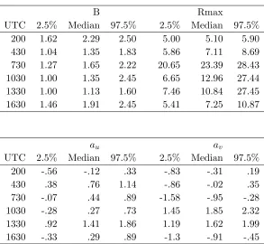
2.1 Posterior medians and 2.5 and 97.5 percentiles for the Holland function and

bias parameters in the separable LMC spatial model foru and v. . . 42

2.2 Deviance Information Criterion (DIC) values for Hurricane Charley data. . . 44

2.3 Model choice results for each time period using Models 1, 2, 3 and 4. . . 44

2.4 RMSPE for V (m/s) based on 30 cross validation sites using the Holland

model output (fixed parameters), fully Bayesian prediction and the empirical

Bayesian approach based on the non–spatial model (Model 1) and separable

LMC model (Model 3). . . 49

3.1 BIC for each time period using Models 1, 2 and 3. . . 74

1.1 Scientific framework for coastal ocean prediction. . . 4

1.2 Bathymetry for model domain. . . 8

1.3 EnsKF with Inundation model. . . 17

1.4 Hypothetical Networks. . . 18

1.5 EnsKF Experiment 1. . . 20

1.6 EnsKF Experiment 2. . . 21

2.1 U-V wind decomposition . . . 28

2.2 Model framework for wind components . . . 32

2.3 Wind contours (m/s) for August 14th hour (i) 200 UTC, (ii) 430 UTC, (iii) 730 UTC, (iv) 1030 UTC, (v) 1330 UTC, (vi) 1630 UTC. . . 40

2.4 Cross validation calibration plots. . . 46

2.5 Map of 2 NBDC buoys within the POM domain. Time series of observed and predictedv winds using Holland output and Model 3. . . 47

2.6 Cross validation time series plots. . . 50

2.7 Map of 7 coastal water elevation gauges and the track of Hurricane Charley. Time series plots os observed and predicted water elevation at each site. . . . 52

2.8 Boxplots of residuals for control run, EnsKF results and output based on LMC winds. . . 53

(iii) 1330 UTC, (iv) 1630 UTC, (v) 1930 UTC, (vi) 2230 UTC. . . 70

3.3 Residualu winds (observed – estimated) in four subregions. . . 71

3.4 Partial autocorrelation for v winds at 6 buoy locations. The time interval is

10 minutes. . . 72

3.5 Posterior distributions for (i) the sill parameter, (ii) the range parameter for

700 UTC. . . 74

3.6 Map of 2 NBDC buoys. Time series of observed and predictedv winds using

nonstationary LMC model. . . 76

Data Assimilation for Coastal Ocean Prediction

1.1

Introduction

Multivariate spatial statistical problems are prevalent in the environmental sciences,

particu-larly in atmospheric and oceanic data applications. In these cases the state space is typically

of very high dimension and the processes of interest are inherently nonlinear and dynamic.

Different sources of information for these systems include observational data as well as

numer-ical models which are based on the fundamental physnumer-ical principles driving atmospheric and

oceanic processes. Over the past decade there has been an increase in the amount of available

real time observed oceanic data as well as advances in the sophistication and resolution of

deterministic ocean models. Whether the state variables of interest are directly observed (e.g.

buoys and ship data) or indirectly observed (e.g. satellite data), these observations may be

at very different scales in space and time. Our goal is to obtain more accurate prediction

of wind fields to improve the quality of storm surge forecasts for the Eastern US coastal

region. These forecasts can be used for assessments of warnings and evacuation notices and

can provide valuable information for recovery operations and response planning.

In order to use all available coastal observations we use data assimilation (DA) which is

the process of combining noisy observations with numerical ocean model output. Multivariate

spatial–temporal modeling techniques are applied to better model hurricane wind fields that

combine wind information from buoys, ships, satellites, and physical models. These wind

fields are used as the primary forcing for numerical forecasts of the coastal ocean response to

In the following sections of this chapter we introduce the concept of data assimilation

and describe a case study for Hurricane Charley of August 2004. In Chapter 2 we propose a

Bayesian framework to capture different sources of uncertainty and bias in available observed

wind data and physics–based wind models. A spatial linear model of coregionalization (LMC)

is used to explain variability in the horizontal and vertical wind components as well as the

cross–dependency between these two components. These methods are then compared with

the Ensemble Kalman Filtering methods to explore the impact on storm surge forecasts for

the same case study of Hurricane Charley. In Chapter 3 we review multivariate spatial

models and propose a new flexible multivariate nonstationary spatial–temporal statistical

model based on an extension of the LMC approach. We conclude with an application to

wind fields from Hurricane Floyd of 1999.

The following chapter is organized as follows. Section 1.2 describes the storm surge

application, the available observed data and the numerical ocean model. Section 1.3 reviews

the sequential Kalman Filtering methods including the Ensemble Kalman filtering technique

proposed by Geir Eversen (Evensen, 1994) that is used here. Section 1.4 describes the results

of a case study of Hurricane Charley of August 2004. In a series of simulations we use model

generated “pseudo” observation to test the effectiveness of the EnsKF approach under two

different sources of modeling error: errors in initial conditions and errors in the surface forcing

fields. We also test the benefit of additional water gauge sites along the coast of Georgia and

the Carolinas by using a set of existing and hypothetical networks. A concluding discussion

1.2

Data and Scientific Problem

1.2.1 Data Assimilation for Storm Surge Forecasting

Storm surge is the abnormal rise of water in the coastal ocean, estuaries and lakes caused

by the high winds and to a lesser extent the low pressure associated with a hurricane or

extratropical cyclone. Storm surge can compound the effects of inland flooding caused by

rainfall, leading to loss of property and loss of life for residents of coastal areas. Historically

storm surge has been responsible for the largest loss of life and property damage since the

effects of the flooding can last long after the hurricane has passed (Powell and Houston,

1996). In order to improve storm surge forecasts data assimilation methods are used to

combine output from a numerical ocean model with coastal observations of the storm surge

height zero to six hours before a hurricane makes landfall.

Clearly, numerical ocean models are essential forecasting tools for coastal areas most likely

to be impacted by storm surge. These models are also used for creating “nowcast” estimates

which are forecasts for short time scales typically less than one hour. However model errors

are inevitable due to uncertainty in initial and boundary conditions as well as simplified or

neglected physical processes or mathematical approximations used in the system equations.

On the other hand, unlike numerical weather prediction applications, available coastal ocean

observations are relatively sparse and may not always capture complex coastal dynamics

(Echevin et al., 2000). Measurement error is also a source of variability that is often not well

understood and so hard to characterize.

Data assimilation (DA) is the process of combining noisy observations with output from

physics–based numerical models. The problem of data assimilation for the oceanic and

at-mospheric sciences fits naturally into a Bayesian framework. That is, we observe data based

on the underlying (unknown) state of the atmosphere or ocean and we estimate this current

Inputs to initialize model (ele,currents,temp,etc.)

Statistical Framework

(physics+space–time model) (Forcing fieldswind f ields)

Numerical Ocean Model (P OM)

Observations

(water level stations,buoy, satellite)

Filtering Methods

(EnsKF)

Nowcast

Final Forecast

? ?

-6

@ @ R

-?

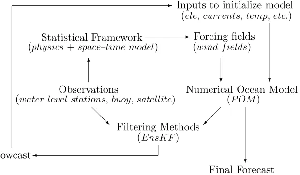
Figure 1.1: Scientific framework for coastal ocean prediction.

mainly been developed for applications in numerical weather prediction. Only in the past

decade has interest begun to grow in applying these data assimilation methods to oceanic

modeling. The main impetus for this new area of research is the substantial increase in the

type and number of observations available for the coastal and open ocean including the

ex-pansion of permanent monitoring networks, the development of lagrangian ocean data and

satellite observations. This observed data can also be used in separate stages of data

assimi-lation as shown in the flow chart in Figure 1.1. Observations can be used to estimate input

fields or optimize parameter values that are used to initialize the numerical model. This step

is the topic of Chapter 2. The focus of this chapter is on the filtering methods that combine

model output with observed data.

In the 1980s and early 1990s several studies were done to test different oceanic DA schemes

in relatively simple models with limited physics. More recently work has been done using

primitive equation models with realistic topography. In a series of papers, Mellor and Ezer

described the assimilation of satellite–derived sea surface data into the Princeton Ocean

Model (POM), a three dimensional ocean model, using an optimal interpolation (OI) scheme

uses a predetermined and fixed (in time) error covariance. Implications of using a fixed error

covariance will be discussed in section 1.3.

Over the past decade more advanced DA methods have been tested for variety of

ap-plications. Evensen and van Leeuwen (1996) used the Ensemble Kalman filter (EnsKF) to

assimilate satellite data into a two layer quasi–geostrophic model for a region off the coast of

South Africa. Verlaan and Heemink (1997) proposed a Reduced Rank Square Root Kalman

Filter (RRSQRT KF) to do tidal flow forecasting using a two dimensional shallow water

equation model. Madsen and Canizares (1999) compared results from the RRSQRT KF and

EnsKF using simulated surface elevation observations (i.e. model generated data plus noise).

They found the RRSQRT KF was more efficient in correcting model errors except in the

case of strongly non–linear dynamics. Echevin et al. (2000) used POM under an idealized

setup with a baroclinic current flowing onto a coastal shelf. They compared two OI methods

with an Ensemble Kalman Fitler (EnsKF) and showed how the impact of assimilated

mea-surements on the analysis is dependent on the location of the observations relative to the

coastline and topography. Luong et al. (1998) used a 4D variational approach to assimilate

satellite derived sea–surface heights into a quasi–geostrophic ocean circulation model.

In terms of data assimilation for storm surge forecasts, Heemink et al. (1997) looked at

forecasts using the KF and the RRSQRT KF. Canizares et al. (1996) and Canizares et al.

(1998) used a 2D shallow water model to apply the RSQRT KF with correlated system noise.

They compared the DA results for a 1993 storm using observations from 9 stations often

impacted by storm surge along the coast of the North Sea.

In this chapter, a sequential data assimilation approach is utilized to improve the quality

of storm surge nowcasts and forecasts for the Eastern US coastal region. These storm surge

estimates can be used for assessments of warnings and evacuation notices and can provide

valuable information for recovery operations and response planning. This is one of many

relies on properly identifying and quantifying disparate sources of uncertainty in the data

analysis. For example, it is often unclear whether the main source of prediction errors is

simplified or neglected physical processes used in the numerical model, inaccuracies in the

initial conditions or errors in the forcing fields. Prediction errors can certainly arise from a

combination of these factor but the challenge is to decide how to allocate time and computing

resources.

Our ultimate goal is to develop methods that would be practical (in terms of computing

time) for real–time forecasting. The sophistication of any proposed methodology must be

constrained by the computing demands of the method. We explore what will have the largest

impact on real–time estimation of coastal water levels under hurricane forcings.

1.2.2 Princeton Ocean Model

The Princeton Ocean Model (POM) is used for coastal ocean modeling, which is adopted by

the National Oceanic and Atmospheric Administration (NOAA) as the operational coastal

ocean forecasting system for the U. S. East Coast. POM is a fully three–dimensional

nu-merical model and has the capability of modeling the evolution of ocean processes at many

layers. In addition, POM uses a bottom following sigma coordinate system to account for

differences in water depth. As a result, the POM model is able to predict storm surge with

greater accuracy than traditional depth–averaged storm surge models (Peng et al. (2004);

Pietrafesa et al. (1997)).

Specifying the bathymetry of the coastal region being studied plays an important part in

storm surge forecasting. According to the Federal Emergency Management Agency: “The

level of surge in a particular area is also determined by the slope of the continental shelf.

A shallow slope off the coast will allow a greater surge to inundate coastal communities.

Communities with a steeper continental shelf will not see as much surge inundation, although

a higher resolution to capture such smaller scale phenomena is essential for improving the

accuracy of coastal forecasts. POM has been used in various applications to model estuaries

and bays, semi–enclosed seas and coastal regions around the world and has been applied

extensively for studies in the Gulf Stream region (see Ezer and Mellor (1997) and references

therein). It has been designed to represent ocean phenomena of 1–100km length and tidal–

monthly time scales. For more details on the governing equations and parameterizations used

in the Princeton Ocean Model see Blumberg and Mellor (1987).

For the case study presented here POM is used to simulate the coastal ocean response to

strong hurricane forcing conditions along the coast of the Carolinas and Georgia. The ocean

model is run at a resolution of 1 minute longitude by 1 minute latitude (_≈ 1.5 km by 1.9

km) using an inundation model developed by Xie et al. (2004) and applied to the Pamlico

Sound system by Peng et al. (2004), that allows for flooding and drying in shallow coastal

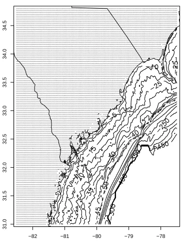
areas. Bathymetry for this gridded domain is obtained from the National Geophysical Data

Center’s (NGDC) Coastal Relief Model as shown in Figure 1.2.

1.2.3 Real Time Water Level Observations

Observed water levels were used from a series of coastal water level stations maintained by

NOAA’s National Ocean Service (NOS) Center for Operational Oceanographic Products and

Services (CO–OPS) as well as those maintained by the Carolina Coastal Observation and

Prediction Program (Caro–COOPS). The state variable of interest is the change in surface

water elevation from an initial value of zero meters which is used for storm surge forecasting.

Hourly data is obtained from 7 coastal sites for Hurricane Charley based on the reported

meters above mean lower low water (MLLW). The MLLW is the average of the lower low

water height of each tidal day observed over a period of 19 years and is used to adjust for

differences in tidal gauge locations.

hurri-−82 −81 −80 −79 −78

31.0

31.5

32.0

32.5

33.0

33.5

34.0

34.5

Figure 1.2: Bathymetry (in meters) for model domain.

cane wind forcing, tidal predictions are also pulled from CO–OPS website. The assimilated

observations are thus the adjusted water level: meters above MLLW minus the predicted

hourly tides. These adjusted observations represent the change in water elevation that can

be attributed to storm surge and in this way can be compared to the state variable in the

numerical model. An alternative approach would be to use a coupled tide–surge model that

includes the tidal signal in the integration of the numerical model (e.g. Jones and Davies

1.3

Coastal Ocean Data Assimilitaion

1.3.1 Kalman Filter

Data assimilation is a type of state space estimation problem where we estimate the state of

a system that changes over time using noisy observations made on the system. Following the

notation of Ide et al. (1997), Yo(ti) = Y_io is a (p_×1) vector of observations at irregularly

spaced points at timeti and X_if is a (n×1) vector consisting of the numerical model output

for k model variables at j grid points in 2 or 3 dimensions at time ti. These variables are

ordered by grid point to form a single vector such that k_×j=n. The true unobserved state

vector X_it is a (n_×1) vector representing the true values of the k variables discretized at

the j model grid points. X_ia will be used to denote the estimated or “analysis” state vector

based on all available observations at timeti.

The evolution of the dynamic system is described by the state or system equation:

X_it=_Mi−_1,i[X_it−1] +ηi (1.1)

where_Mi−_1,i[] represents the forward integration of the current state by the numerical model.

The observation equation relates the observations to the state vector in the presence of

measurement error:

Y_io =_Hi[Xit] +ǫoi (1.2)

Hi[] is the observation operator which interpolates the model variables to the observation

locations and transforms the model variables to the observed variables. It is typically assumed

ǫo

i ∼Po(0, Ri),ηi ∼Pf(0, Qi) and Cov(ǫoi, ηi) = 0. In the case thatǫo

i andηiare normally distributed andHi[] andMi−_1,i[] are linear

opera-tors,Hi(n×_p),Mi−_1,i(n×_n), an analytic solution exists for the posterior distribution of the true

state conditioned on available data. Prior to observingY_io, the numerical model represented

the estimated state vector and error covariance matrix from the last time period, (Xa i−₁,

Pa

i−₁), the prior distribution is:

P(X_it_|Y_io−₁)∼N(X

f i, P

f

i ) (1.3)

where

X_if =Mi−_1,iX_ia−₁

P_if =Mi−_1,iP_ia−1M

T

i−1,i+Qi

(1.4)

This forecasting step is what makes the Kalman Filter so computationally expensive.

The matrix multiplication by Mi,i+1 to obtain the forecast error covariance Pif+1 requires

approximately as much computing effort as advancing the the deterministic forecast model

n/2 times where n, the dimension of the state vector, is typically on the order of 103 – 105 (Kalnay, 2003).

Note thatP(Y_io_|X_it, Y_io−₁) =P(ei|X

t

i, Yio−₁), whereei is the difference between the

obser-vation and the first guess obtained by applying the obserobser-vation operator Hi to the current

forecast, ei = Yio−HiX_if. This is known as the observation increment. Since Hi, Mi−1,i,

and Xa

i−1 are known, observingY

o

i is equivalent to observing ei. Hence the likelihood is

P(ei_|X_it, Y_io−₁)∼N(Hi(X

t

i −Xif), Ri) (1.5)

An estimate of the current state of the atmosphere based on the observation and state

equa-tions described above can be easily obtained by a direct application of Bayes Theorem

(Mein-hold and Singpurwalla, 1983). Given the prior distribution P(X_it_|Y_io−₁) and the likelihood

L(X_it_|Y_io) = P(Y_io_|X_it, Y_io−₁) then the posterior conditional distribution best describing the

state of the atmosphere at time ti based on all available data is given by,

P(X_it_|Y_io, Y_io−1) =

P(X_it_|Y_io−₁)×P(Y

o

i |Xit, Yio−₁)

R

P(Xt

i, Yio|Yio−1)dX

t i

(1.6)

For Gaussian prior and likelihood distributions a standard multivariate result (see

this result the joint distribution for ei andXit is:    ei

X_it

  

Y_io−₁

∼N    0

MiX_ia−₁

  ,   

Ri+HiPifHiT HiPif

P_ifH_iT P_if



 

(1.7)

Thus the posterior conditional normal distribution is:

P(X_it_|ei, Yio−₁) = (X

t

i|Yio, Yio−₁)∼N(MiX

a

i−₁+Ki(Y

o

i −HiXif),(I−KiHi)Pif) (1.8)

where Ki is the Kalman gain matrixKi =P_ifHiT(Ri+HiP_ifHiT)

−₁

.

Now the updated estimate for the current state vector (the analysis vector) is simply the

posterior mean:

X_ia=X_if+Ki(Yio−HiXif) (1.9)

and the updated forecast error covariance matrix equals the posterior covariance matrix:

P_ia= (I₋KiHi)Pif (1.10)

This pair, (Xa

i, Pia) is then used in the prior distribution (1.3) to initiate the next fore-casting/updating cycle for timeti+1. Notice that the Kalman gain matrix will be larger when

the forecast error covariance P_if is large compared to the observation error covarianceRi. In

turn, the larger Ki matrix in (1.9) will mean a larger correction to the “first guess” vector

X_if.

In data assimilation applications in the geophysical sciences the state vector of interest

is of very high dimension and the dynamic systems being modeled are typically nonlinear.

Nonlinear processes are especially important for coastal dynamics due to the complexities of

local bathymetry and coastlines and the influence of wind forcings, tides, and storm surge.

As a result the numerical model_Mi−_1,iis typically a nonlinear function of the state variables

and the normality assumption for the error terms may not be realistic. The Extended Kalman

observation operators. The ExKF has historically been found to be effective for weakly

non-linear systems but the computational demands of propagating the error covariance forward

in time, seen in the KF, still remain.

It is relevant to note that Optimal Interpolation, mentioned in section 1.2 uses the same

updating formulas as the KF. The difference in the two methods is that the OI scheme

assumes the background error covariance is fixed in time so that P_ia=Pa is estimated once

prior to the DA cycle rather than evolving in time as in the Kalman filtering methods.

1.3.2 Variational Methods

Kalman filter approaches are known as a type of sequential method due to the fact that if

measurement error is assumed to be uncorrelated, it is possible to assimilate observations one

at a time as they become available. Briefly we mention an alternative type of approach to

data assimilation, known as variational methods. Variational methods build from Bayesian

optimal control theory and utilize a cost (or risk) function, J(X), to minimize the distance

between the model output and a set of measurements within a given time interval. Specifically,

the 3D–Var approach finds the value of the state vector X that minimizes the distance to the

background state and to the observations (each weighted by their inverse error covariances)

using a quadratic cost function:

2J(X) = (X₋Xb)TB−₁

(X₋Xb) + (Yo₋H(X))TR−₁

(Yo₋H(X)) (1.11)

In fact, for Gaussian model and observation errors, the solution to this minimization problem

is precisely the maximum likelihood estimator. Thus it can be shown (e.g. Kalnay (2003),

pg 171) that Optimal Interpolation (a sequential method) and 3D–Var are solving the same

problem.

As in optimal interpolation, 3D–Var methods use a predefined error covariance that

is particularly unrealistic in coastal ocean modeling where the dynamics of the system are

“strongly influenced by land–sea boundaries and the flooding and drying of tidal areas”.

This is why more advanced methods such as the Kalman filter and it variants, are much

more attractive for oceanic applications.

A more advanced variational method, 4D–Var, also accounts for the dynamic propagation

of model errors. J(X) in 4D–Var is a function of the distance to the background at the start of

the assimilation window, i.e. X(t0)−Xb(t0). The minimization of the cost function requires a

linear tangent model which is the linearized Jocobian (L(t0, ti) =∂Mi/∂X0) and its adjoint

(LT_(t

i, ti−₁)) which takes gradient information backwards in time. The solution to 4D–Var

is a new “optimized” initial state X0 which is integrated forward by the model to form the

analysis at time ti: Xa(ti) = M0,i[X0]. 4D–Var does not require the model to be a linear

system since it utilizes the linear tangent and adjoint models but is does assume that the

dynamical model is perfect.

4D–Var is typically much more computationally expensive than the Ensemble Kalman

filter methods. It also requires the development of the linear tangent and adjoint models

which will be unique for each numerical model. In the realm of numerical weather prediction

it is still unclear which method performs better for forecasting. In oceanic data assimilation

the comparisons between these two methods are still in their very early stages.

1.3.3 Ensemble Kalman Filter

A common adaptation of the KF is the Ensemble Kalman Filter (EnsKF) proposed by Geir

Eversen in 1994 which uses a Monte Carlo approximation of the forecast distribution. The

Ensemble Kalman Filter approach is used to generate samples of the state vector and carry

out an ensemble of data assimilation cycles. This ensemble is then used to estimate the

analysis mean and error covariance. The EnsKF uses the following algorithm where the

Forecast Step:

1. Sample X_i(−j)₁ ∼P(X

a i−1, P

a

i−1), j= 1, ..., Ns

2. Compute X_if(j)=_Mi−_1,iX

(j)

i−₁,j = 1, ..., Ns

3. Calculate sample mean and covariance:

ˆ X_if = 1

Ns Ns

X

j=1

X_if(j)

ˆ

P_if = 1 Ns−1

Ns

X

j=1

[X_if(j)₋Xˆ_if][X_if(j)₋Xˆ_if]T

(1.12)

Analysis Step:

1. Perturb the observations at time ti by adding random noise (typically Gaussian):

Y_i∗(j)=Yo i +η

(j)

i , η

(j)

i ∼N(0, Ri), j= 1, ..., Ns

2. Update each member of the forecast sample with the KF analysis step:

X_i(j)=X_if(j)+Ki(Y_i∗(j)₋HX_if(j)),j = 1, ..., Ns Ki = ˆP_ifHT(Ri+HPˆ_ifHT)−1

3. This now serves as a sample for time ti and the process repeats.

Typically ensembles of only 10 to 100 members are used to approximate the first two

mo-ments of the update distribution. The EnsKF requires considerably less computational cost

compared to the Extended Kalman Filter and it avoids problems associated with the

lin-earization of the forecast model. It has been found that these sample estimates tend to

underestimate the forecast error covariance. It can be shown that for the case of linear

dy-namic and observation operators and Gaussian errors for large ensemble size, Ns, the update

update formulas derived from these assumptions there is no theoretical justification that the

updated sample from the EnsKF will be representative of the true state for nonGaussian

error statistics. On the other hand, the EnsKF clearly has an advantage over OI and 3D Var

methods that use a constant error covariance since it allows for the nonlinear evolution of

the error statistics.

1.4

Ocean Model Application: Hurricane Charley

1.4.1 An EnsKF for Assimilation of Water Level Observations

In this section the Ensemble Kalman Filter is applied to a case study of Hurricane Charley

of 2004. This case study was chosen because the hurricane surface winds induced

consider-able storm surge within the CaroCOOPS observing array off the coast of Georgia and the

Carolinas. Storm surge predictions based on a control run of the ocean model are compared

to the analysis output from the EnsKF and to the observed data.

Hurricane Charley crossed over the central Florida peninsula and moved offshore early on

the morning August 14th, 2004. Charley made landfall at Cape Romain, SC at 1400 UTC

(Coordinated Universal Time) on the 14th as a weakening Category 1 storm with highest

winds around 80 miles per hour (70 kt/hr). It moved off shore again and then made landfall

a few hours later at North Myrtle Beach, SC. Water level gauges along the coast of Georgia

and the Carolinas reported storm surge heights up to 1.5 meters above normal tidal levels.

The Tropical Prediction Center of the NHC reports that Charley caused insured damages of

25 million dollars in North Carolina and 20 million dollars in South Carolina.

An axis–symmetric wind model (Holland, 1980) is used to initialize POM based on track

information available from NOAA for the center location and central pressure of Hurricane

Charley on August 13th – 15th. The Holland model has two forcing parameters, Rmaxand

of the pressure profile. These parameters are chosen based the size and intensity of the storm

(Rmax= 46; B = 1.9) using an approach suggested by Hsu and Yan (1998). See Xie et al.

(2006) and Peng et al. (2004) for further details on surface wind forcings and storm surge

forecasting for coastal ocean systems. The Holland model will also be dicussed in further

detail in Chapter 2.

The state variable of interest is the change in surface water elevation (storm surge).

A statistical ensemble of initial elevation fields is generated using a Gaussian random field

centered at zero meters with an exponential spatial covariance model. The ocean model is

run at a resolution of 1 minute longitude by 1 minute latitude with four layers of 301_×229

grid points. Due to the computational cost of using such a high resolution we use an ensemble

size of twenty. The analysis/forecast cycle is initiated using a 12 hour “spin–up” from August

13, hour 900 UTC to August 14, hour 900 UTC to simulate the sea state conditions along

the Eastern coast leading up to the data assimiliation window (i.e. the time period six hours

prior to landfall).

From August 14th, 900 UTC to August 14th, 1800 UTC the EnsKF is used to update the

state vector every hour using observed data from 7 water level stations in North Carolina,

South Carolina and Georgia within the model domain. The observation error is assumed to

be independent with error variance for each site based on the reported one second variability

in the water level values.

Figure 1.3 shows the observed water levels at each of the 7 water gauge sites as Hurricane

Charley moves along the coast. The Sunset Beach site shows the greatest storm surge of 1.67

meters. The dashed and dotted line shows the ocean model output of surface elevation based

on the control run without DA. This control run tends to overestimate the increasing and

decreasing elevation values and also exaggerates the effects of the hurricane on the coastal

sites at Charleston, SC and Fort Pulaski, GA which exhibit little to no storm surge during

−82 −80 −78 −76 −74 31 32 33 34 35 36 Wrightsville Beach Sunset Beach Springmaid Pier Oyster Landing Charleston Fort Pulaski St. Simons Island

−82 −80 −78 −76 −74

31 32 33 34 35 36

Hurricane Charley Track: August 14th, 2004

9 10 11 12 13 14 15 16 17 18

10 12 14 16 18

−1.5 −1.0 −0.5 0.0 0.5 1.0 1.5

(i) Wrightsville Beach

Aug. 14 UTC

change in surface elevation

−−−−−−−−−−−− Observed

− − o − − o − − Control

−−o−−o−−o−− Ensemble Mean

10 12 14 16 18

−1.5 −1.0 −0.5 0.0 0.5 1.0 1.5

(ii) Sunset Beach

Aug. 14 UTC

change in surface elevation

10 12 14 16 18

−1.5 −1.0 −0.5 0.0 0.5 1.0 1.5

(iii) Springmaid Pier

Aug. 14 UTC

change in surface elevation

10 12 14 16 18

−1.5 −1.0 −0.5 0.0 0.5 1.0 1.5

(iv) Oyster Landing

Aug. 14 UTC

change in surface elevation

10 12 14 16 18

−1.5 −1.0 −0.5 0.0 0.5 1.0 1.5 (v) Charleston

Aug. 14 UTC

change in surface elevation

10 12 14 16 18

−1.5 −1.0 −0.5 0.0 0.5 1.0 1.5

(vi) Fort Pulaski

Aug. 14 UTC

change in surface elevation

10 12 14 16 18

−1.5 −1.0 −0.5 0.0 0.5 1.0 1.5

(vii) St. Simons Island

Aug. 14 UTC

change in surface elevation

−82 −81 −80 −79 −78

31

32

33

34

Network 1: Caro−COOPS Sites

−82 −81 −80 −79 −78

31

32

33

34

Network 2

−82 −81 −80 −79 −78

31

32

33

34

Network 3

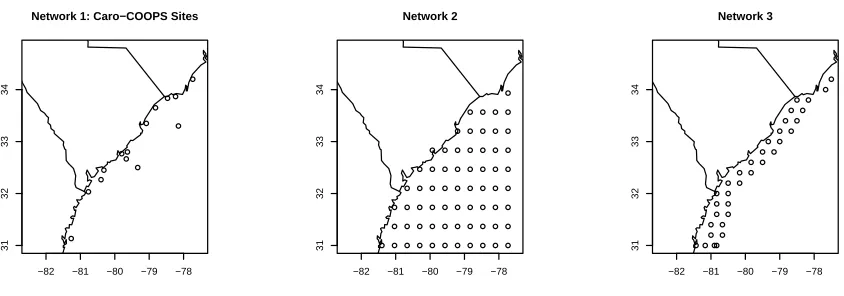
Figure 1.4: Hypothetical networks 1, 2 and 3 in ocean model domain. Network 1 includes existing locations of Caro–COOPS and CO–OPS moorings and water level sites.

times and is plotted as a dotted line. The EnsKF adjusts the model output and reduces

prediction error when compared to the control run. The ensemble mean better captures the

magnitude and the timing of the peak surge at these sites. This improvement is most notable

at the Oyster Landing and Charleston sites. However both control run and EnsKF analysis

output underestimate the largest surge value at the Sunset Beach location.

1.4.2 EnsKF Twin Experiments

We now investigate whether errors in initial conditions or in wind forcing parameters play

a larger role in hurricane storm surge forecasting. The Ensemble Kalman Filter adjusts

the estimate of the state vector X_it which is then used as the new initial conditions for the

subsequent forecast. If model errors are more influenced by errors in the forcing fields we

may wish to concentrate computing time on improving estimates of the surface wind fields

rather than correcting errors in the initial conditions. We conduct a series of identical twin

experiments meaning the model is assumed to be perfect. “Psuedo” observations are used

for the data assimilation step, i.e. model generated data plus simulated measurement error.

In the first set of experiments the true state is defined as model generated output for

hours 900 UTC to 1700 UTC, August 14th, based on a model run with a 12 hour spin–up

from August 13 hour 900 UTC to August 14th hour 9 UTC. The control run is then model

output for this 9 hour period based on a model run with no spin–up. In other words, the

“true” initial elevation fields for hour 900 UTC are simulated by POM based on 12 hours

of hurricane force winds, but our control run assumes that the initial elevation fields are

uniformly zero at this hour. Under this set–up, the impact of adding additional water level

gauges within the model domain of interest is also tested. Figure 1.4 depicts three monitoring

networks along the coast of the Carolinas and Georgia. Network 1 includes existing CO–

OPS locations as well as moorings and water level sites from the Carolinas Coastal Ocean

Observing and Prediction System (Caro–COOPS). The remaining two hypothetical networks

are used to study the impact of additional sites by comparing the difference in adding these

sites evenly throughout the domain (Network 2) versus concentrating the new sites along

the coast (Network 3). It is not expected that such a large number of extra sites would

ever realistically be used but this exaggerated design is used to help determine the benefit of

additional water gauge sites and to evaluate the effectiveness of the current network.

Based on pseudo observations from the true model run at each observation network the

Ensemble Kalman filter is used to assimilate the noisy (i.e. including measurement error)

hourly water elevation values at hours 900 UTC to 1400 UTC. The model is then integrated

forward without the benefit of DA for a three hour forecast from 1500 UTC to 1700 UTC.

Since we are typically most interested in the areas along the coast with the greatest amount

of storm surge we compare the prediction errors (observed water level – predicted water level)

at only 10% of the surface grid points where the largest increase in the true elevation values

is observed (i.e. there are a total of 17365 surface layer grid points and we consider the errors

at 1736 locations near the coast).

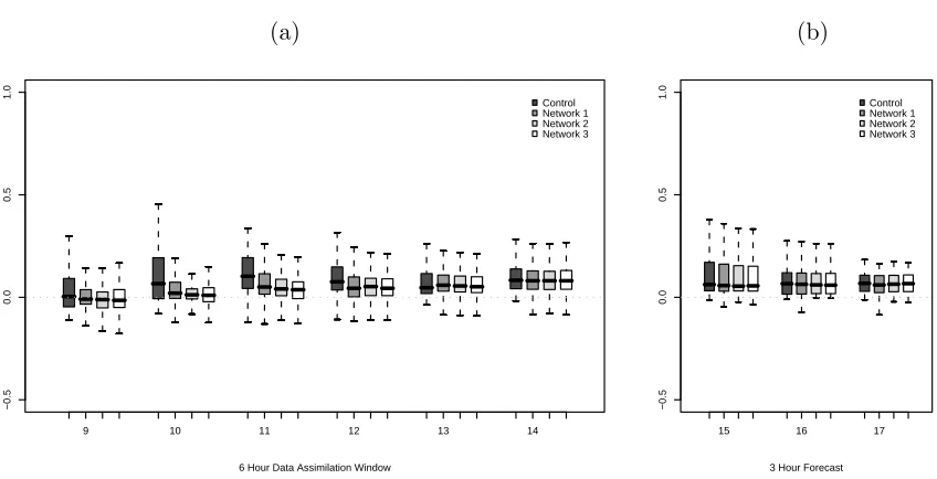
(a) (b)

9 10 11 12 13 14

−0.5

0.0

0.5

1.0

6 Hour Data Assimilation Window

Control Network 1 Network 2 Network 3

15 16 17

−0.5

0.0

0.5

1.0

3 Hour Forecast Control Network 1 Network 2 Network 3

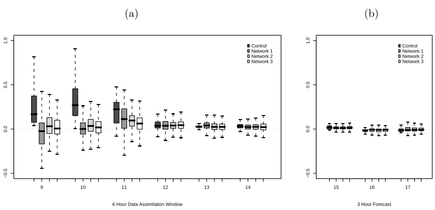
Figure 1.5: Boxplots for prediction errors (in meters) under Experiment 1 (a) for DA cycle August 14 900 UTC to 1400 UTC, (b) for 3 hour forecast from 1500 UTC to 1700 UTC.

the three network designs for the six hour DA cycle. At the beginning of the DA cycle there

are prediction errors up to 1 meter in the control run. During this time the control run

exhibits large bias (the median bias is depicted by the bar in the center of each boxplot).

The DA estimates are less biased and show less error variance as well. Although there is

some reduction in the model errors based on the DA using the different network designs, this

improvement is only evident at the beginning of the DA window. Even Network 2 which has

65 locations does not greatly reduce prediction errors after the third hour when compared to

the Network 1 with only 14 sites. The errors in the control and the DA output decrease over

time. Both the true model run and the control run used the same wind forcing fields. Errors

in the initial elevation does not appear to have a lasting impact on the prediction of surface

elevation in this scenario. For the three hour forecast shown in Figure 1.5(b) there is little to

no remaining effect of using the incorrect initial conditions at hour 900 UTC and all of the

forecast values are very close to the true elevation at these times.

(a) (b)

9 10 11 12 13 14

−0.5

0.0

0.5

1.0

6 Hour Data Assimilation Window

Control Network 1 Network 2 Network 3

15 16 17

−0.5

0.0

0.5

1.0

3 Hour Forecast Control Network 1 Network 2 Network 3

Figure 1.6: Boxplots for prediction errors (in meters) under Experiment 2 (a) for DA cycle August 14 900 UTC to 1400 UTC, (b) for 3 hour forecast from 1500 UTC to 1700 UTC.

14th, is defined as model output based on a model run using a 12 hour spin–up under forcing

fields with Rmax= 46 and B = 1.9. For the control run we treat these “true” parameters

as unknown and fix Rmax = 35 and B = 1.0 indicating a much weaker storm. We repeat

the DA/Forecast cycles as before for the three observation networks. The boxplots of the

prediction errors are given in Figures 1.6(a) and (b). In this experiment we see the model

error increases over time as the hurricane eye moves into the model domain and then decreases

at hour 17 UTC as Charley moves inland and the surface wind induced storm surge is greatly

reduced.

Even though the EnsKF is correcting initial conditions not errors in the forcing fields,

these plots show some improvement in prediction during the six hour DA window. The

improvement is much less during the three hour forecast cycle. Again there is not a significant

difference between the results based on the three different observation networks. In general

the additional observation locations do not have much impact on reducing model error when

estimates in the control run. As expected the predicted values tend to be smaller than the

true values due to the incorrect specification of the wind forcing fields. As this error in the

forcing fields persists over time the data assimilation results do not fully correct this bias.

This is especially true for the forecasting errors which are almost all positive for the control

run as well as the DA estimates. This suggests that improvement in the wind forcing fields are

needed to achieve improved forecasts. As shown in Figure 1, wind observations can also be

used in the DA cycle through inverse modeling techniques or statistical modeling to improve

the method of calculating these input fields. This issue is further explored in Chapter 2.

1.5

Discussion

In this chapter we considered data assimilation results for real–time estimates or nowcasts

of hurricane induced storm surge. We found we were able to improve the output from

the numerical ocean model at times when observational data is available. A separate but

very important issue is the impact of data assimilation on forecasts. In this case the data

assimilation results are used as improved initial conditions when the ocean model is integrated

forward. Our analysis of these forecasting results through the identical twin experiments show

that the forecast ensemble mean follows the control run after only a few hours. This suggests

information from the observed water level is propagated to the state variables of the numerical

model only during the assimiliation window. As a result the forecast storm surge predictions

do not show an improvement over the control run except for short term nowcasts.

We test the effect of the choice of the ensemble size and the values of the error covariance

used to create the initial ensemble of perturbation fields. Using a lower resolution ocean

model we run the data assimiliation analysis with 80 ensembles as well as 20 and find very

little difference in the ensemble mean values used for prediction. We also vary the spatial

different values for the parameters of the exponential covariance formula. We find these

changes also have very little impact on the final analysis fields produced by the Ensemble

Kalman filter. Consistently in each data assimilation run the variability or “spread” of the

ensembles quickly decreases during the several hours of forecasting/updating steps. This is

due in large part to the influence of the surface wind forcings driving the ocean model which

is the topic of Chapter 2. In the following chapter we describe a methodology for including

disparate sources of surface wind field data into the data assimilation scheme for coastal

ocean prediction. We shall see that we can also obtain improved storm surge estimates by

Chapter 2

A Bayesian Framework for Multivariate Spatial

Wind Field Prediction

2.1

Introduction

Estimating the spatial and temporal variation of surface wind stress fields plays an important

role in modeling atmospheric and oceanic processes. This is particularly true for hurricane

forecasting where numerical ocean models are used to simulate the coastal ocean response

to the high winds and low pressure associated with hurricanes, such as the height of the

storm surge and the degree of coastal flooding. According to the National Oceanic and

Atmospheric Administration’s (NOAA) Hurricane Research Division more than eighty–five

percent of storm surge is caused by winds pushing the ocean surface ahead of the storm.

The numerical ocean models used for storm surge forecasting are also driven primarily by

the surface wind forcings. Houston and Powell (1994) did an analysis of the impact of wind

field forcings on the storm surge forecasts used by the National Hurricane Center (NHC).

They concluded that up to 6 hours before landfall, real–time model runs can be used to

evaluate warnings and assess the extent of storm surge inundation. Houston et al. (1999)

state that “an accurate diagnosis of storm surge flooding, based on the actual track and

wind fields could be supplied to emergency management agencies, government officials, and

utilities to help with damage assessment and recovery efforts.” Our objective is to use all

available sources of wind data in order to improve the estimation of the wind field inputs. It

is expected that improving these inputs will have a great impact on real–time storm surge

landfall according to the areas most impacted by the storm.

Several studies have investigated the potential of using real–time observation–based winds

to improve storm surge predictions as new wind observations have become available from the

Hurricane Research Division (HRD). Since 1993 the HRD has reported real–time analyses

of tropical cyclone surface wind observations for evaluation and eventually to be utilized by

the NHC (Houston and Powell, 1994). Powell and Houston (1996) did a study of Hurricane

Andrew (1996), and concluded that real–time wind fields would improve storm surge forecasts,

particularly for storms with asymmetric (i.e. non axis–symmetric) wind fields. Houston et

al. (1999) used the HRD winds as input into a two dimensional storm surge model. In their

analysis they did not allow the wind and surface pressure field to change over time, but rather

ran the ocean model assuming the wind and surface pressure fields were steady state for over

24 hours.

We propose a new method to use the HRD data to fit a statistical model for the winds

that can be used as input into a numerical ocean model. The statistically–based winds are a

function of the hurricane’s location and can be updated at intervals as small as 10 minutes as

more observations become available. A statistical framework is used to account for systematic

and random errors in the observations while using these observations to model the surface

winds as a multivariate spatial process. This is the first time that these methods have been

applied to an ocean model application to be used for improved storm surge forecasting.

The statistical modeling of spatial temporal processes in the atmospheric sciences has

been an active area of research over the past decade. Hierarchical Bayesian methods have

been found to be particularly useful for such applications, e.g. see Wikle et al. (1998),

Berliner et al. (1999) and Royle et al. (1999). Such methods have been applied to modeling

wind fields. Wikle et al. (2001) present a hierarchical spatial–temporal model for surface

wind fields over the tropical oceans. Fuentes et al. (2005) propose a method for predicting

for bias in available observations. In both of these studies the orthogonal components of

the vector wind fields are treated as independent. Cripps et al. (2005) apply generalized

autoregressive conditional heteroscedastic (GARCH) models to the bivariate wind vector at

a single spatial location. In our statistical framework we combine all sources of available data

including a physics–based wind model and the observational data currently available to NHC

for coastal ocean prediction along the Eastern coastline. We investigate the importance of

accounting for the cross–covariance of hurricane surface wind fields. The ultimate goal in

the application presented here is to develop methods that would be practical (in terms of

computing time) for a real–time forecast or nowcast scenario. Hence the sophistication of

any proposed methodology must be constrained by the computing demands of the method.

The scientific question of interest is how to balance the sophistication of the wind field model

with computational cost.

Section 2.2 describes the deterministic physical model for surface wind fields, the available

observed data and the proposed statistical model. Section 2.3 reviews statistical methodology

for multivariate data following the linear model of coregionalization used in this paper. We

outline a hierarchical Bayesian approach for estimation of parameters in a deterministic wind

model and prediction of gridded surface wind fields. Section 2.4 describes the results of a

case study for wind field data from Hurricane Charley in August of 2004. The estimated

wind fields are used to initialize the numerical ocean model and are shown to improve storm

surge prediction. A concluding discussion is given in section 2.5.

2.2

Data and Scientific Problem

2.2.1 Modeling Surface Wind Fields

For coastal ocean modeling we use the Princeton Ocean Model (POM), which is a three–

fields are the most important input variable used to initialize the numerical ocean model

to simulate the coastal ocean response to hurricanes. A wind field is made up of wind

vectors defined at a finite set of grid points such that each vector has a magnitude or wind

speed value (typically measured in meters per second or knots) and a direction. These

vectors are decomposed into orthogonal u winds, (East–West) and,v winds, (North–South).

A Bayesian hierarchical framework is used to combine different sources of wind data at

different locations in order to predict the wind fields at the grid locations used by the ocean

model. Let V(s, t) = (u(s, t), v(s, t))T _{be the underlying unobserved spatial process for the}

wind components at location s and time t. The standard Cartesian decomposition is used

to define the wind vectors since the observed and predicted winds provided by NOAA are

based on this decomposition. However we note that other decompositions are possible and

in particular the u andv components could also be defined according to the direction of the

motion of the storm at a given time.

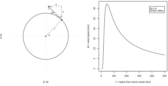
Currently for storm surge forecasting a deterministic wind model is used, referred to as

the Holland wind model (Holland, 1980) which determines the wind velocity induced by the

hurricane pressure gradient under cyclostrophic balance. The Holland wind model for surface

wind speed at a given location s and timetis:

W(s, t) =

"

B ρ

Rmax r

B

(Pn−Pc) exp−(Rmax/r)

B

#1/2

(2.1)

Pnis the ambient pressure, Pc is the hurricane central pressure at timet,ρ is the air density

(fixed at 1.2 kgm−₃

), andr is the distance from the hurricane center to locationsat time t.

Under the assumption that the hurricane wind field is axis–symmetric the u and v

com-ponents can be determined from the wind speed:

uH(s, t) =W(s, t)sinφ (2.2)

E−W

S−N

φ

r

W v

u

φ

0 100 200 300 400 500

0

5

10

15

20

25

30

r = radius from storm center (km)

W = wind speed (m/s)

B=1.9 Rmax=45km

Figure 2.1: U–V wind decomposition for symmetric Holland wind model.

where φ is the inflow angle at site s across circular isobars toward the storm center at

time t. That is, for every location the covariates for u and v are the radius (r), and angle

(φ). The wind components are a nonlinear function of these covariates with parameters

θH _{= (B, Rmax). The forcing parameter Rmax is the radius of maximum sustained wind}

of the hurricane. In the Holland model the maximum possible wind speed in the storm is a

function of the central pressure of the storm and the value B which defines the shape of the

pressure profile. Large values of B correspond to a wind field with very high wind speeds in

a small region near the center of the storm. A smaller B value will mean high wind speeds

across a greater radius of the storm. These parameters are typically based on results from

previous studies and are held constant for all forecasting time periods.

Although this physical model incorporates important information provided by the

ob-served central pressure and the location of the eye of the storm there are known deficiencies

in this formulation. For example, the Holland winds are symmetric around the storm center,

hurri-cane (with respect to the storm movement). Various adaptations of this physical model have

been proposed. Xie et al. (2006) create an asymmetric model by incorporating data provided

by the National Hurricane Center (NHC) guidance on the maximum radial extent of winds

of a given threshold in the four quadrants of the storm. The NHC uses a parametric wind

formula similar to the Holland model to force the ocean model. Another approach would be

to use a coupled atmospheric–oceanic numerical model to simulate the surface winds at the

boundary layer of the ocean model. Global mesoscale numerical weather forecasting

mod-els such as the Mesoscale Model (MM5) and the Weather Research and Forecasting Model

(WRF) are capable of making forecasts for surface level wind fields. However these forecasts

are not suitable for real–time forecasts of hurricane winds. Historically these models have

been unable to accurately reproduce the intensity of hurricane force winds. More recent

re-ports show that MM5 and WRF are able to obtain more realistic wind speeds when run at

high resolution (on the order of 1 km grid size). However the CPU time required to produce

these modeled winds prevents such model runs from being used in real–time applications. The

best approach for regional storm surge forecasting is still using parametric hurricane models,

as discussed in Xie et al. (2006). For further details on storm surge forecasting for the coastal

ocean and estuarine systems see Xie et al. (2004), Peng et al. (2004), and references therein.

Here we focus on the operational methods and observational data currently available

to the NHC for coastal ocean prediction along the Eastern coastline and incorporate this

information into a statistical framework. In our analysis we provide a new tool to estimate

the parameters of the Holland wind function. We include the Holland winds as the mean

function of a spatial statistical model and incorporate a spatial covariance to account for any

structures in observed hurricane surface winds not captured by the parametric wind fields.

This approach to wind field modeling provides parameter estimates and standard errors as

2.2.2 Wind Data

There are three sets of available wind data to be used in hurricane forecasting and hindcasting.

Data provided by the National Hurricane Center (NHC) specifies the location of the storm

center and the central pressure. The NHC provides forecasts every 6 hours on the location

of the hurricane center (in degrees latitude/longitude) and sustained wind speeds (nautical

miles) in different quadrants of the storm. For historical datasets such as these there is also

“best” track information for the hurricane center and central pressure based on all available

observations along the coast. The track information is necessary when creating wind fields

based on the Holland wind model. Linear interpolation is used to interpolate the best track

information to estimate the storm center and central pressure at ten–minute time intervals.

In addition, data on wind speed and direction at over 20 buoy locations along the Eastern

coast is available from NOAA’s National Data Buoy Center (NDBC). For this study we use

the ten minute average wind speed (m/s) adjusted to a common height of 10 meters above

sea level and ten minute average wind direction. Ten minute averaging times are considered

to be representative of the timescales typically associated with oceanic response to surface

stress (Houston et al., 1999). The wind speed and direction are then converted to u and v

components.

Finally, gridded wind field data is available from NOAA’s Hurricane Research Division

(HRD). These wind fields are a combination of surface weather observations from ships, buoys,

coastal platforms, surface aviation reports, reconnaissance aircraft data, and geostationary

satellites which have been processed to conform to a common framework for height (10 m),

exposure (marine or open terrain over land) and averaging period (maximum sustained 1

minute wind speed). The processing and quality control of the data use accepted methods

from micrometeorology and wind engineering and provide the best available near real–time

gridded hurricane wind analyses. However it is important to note that validation studies

quality and quantity of the observations used, and on the appropriateness of the underlying

assumptions used to manipulate the observations. Houston et al. (1999) report the gridded

wind fields have been found to have estimated errors of up to 10%–20%. For this reason

although buoy observations are used to create the HRD wind fields the observed winds from

the NDBC buoy network are also used as a second data source to provide an estimate of

the bias in the HRD analysis fields. For more information on the HRD data see Powell

et al. (1996) and Powell and Houston (1996). HRD data is typically available at 3 hour

intervals. HRD gridded fields are provided at a resolution of approximately 6km _×6km with

the number of grid points on the order of 104_.

2.2.3 Statistical Model for Data

A statistical framework is used to account for the difference in uncertainty associated with

buoy and HRD analysis data. As described in the previous section the observed winds at

the buoys are considered more reliable compared to the HRD analysis data which has been

shown to have potentially large biases. This does not mean that no bias exists in the buoy

data. For example wave distortion effects have been found to result in a negative bias when

deriving wind stress from low–level anemonometers (Large et al., 1995). All of the buoy

observations used in this study have anemometer heights that are at least five meters above

mean sea level. In fact more than half of the sites are at heights greater than ten meters and

so should not be influenced by surface waves. We cannot hope to accurately estimate the

bias of both data sources but only the bias of the HRD data with respect to the buoy data.

We take this approach since past studies suggest that the magnitude of the bias in the HRD

data, which includes satellite and ship data, is larger than the potential bias in the buoys.

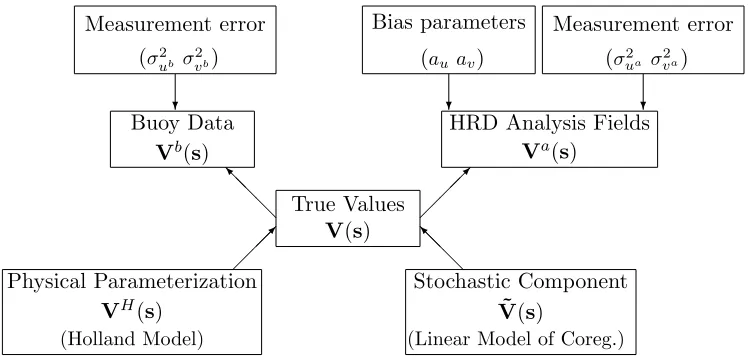
Let Va(s, t) = (va_{(s, t), u}a_{(s, t))}T _{be the u and v components provided by the HRD}

analysis at time t and location s. Let Vb(s, t) = (vb(s, t), ub(s, t))T be wind data from the

Measurement error (σ2

ub σ 2 vb)

Bias parameters

(au av)

Measurement error (σ2

ua σ 2 va)

Buoy Data Vb(s)

HRD Analysis Fields Va(s)

True Values V(s)

Physical Parameterization VH(s)

(Holland Model)

Stochastic Component ˜

V(s)

(Linear Model of Coreg.)

? ? ? @ @ @ I @ @ @ I

Figure 2.2: Model framework for wind components.

The observed data is modeled as a function of the underlying true (unobserved) wind process

V(s) = (u(s), v(s))T. Then V(s) is modeled as a multivariate spatial process with a mean

function equal to the nonlinear parametric Holland formula. This framework is depicted in

Figure 2.2. The data model includes bias parameters,a(s) andb(s), as well as measurement

error terms, ǫb_{(s) and ǫ}a_(s):

ˆ

Vb(s) =V(s) +ǫb(s) (2.4)

ˆ

Va(s) =a(s) +b(s)V(s) +ǫa(s) (2.5)

Here a(s) = (au(s), av(s))T and b(s) =diag(bu(s), bv(s)) are spatial–temporal functions

for additive and multiplicative bias. These may be modeled as polynomial functions of

location, spline functions or as a function of additional covariates such as temperature or

pressure. Based on exploratory analysis comparing the buoy and HRD data we find that a

multiplicative bias term in not necessary and set bu(s), bv(s) = 1 for all locations s. Due to

the limited amount of buoy data we consider only constant bias terms a(s) = (au, av)T for

all locations s.